跳到论文正文
W Papers独立论文阅读器 arXiv:0810.4050 论文正文 计算阅读时间 · 0%
引用这篇论文根据当前论文元数据生成,正式投稿前建议核对。


License: arXiv.org perpetual non-exclusive license
arXiv:0810.4050v2 [cond-mat.stat-mech] 01 Apr 2009

Quantum Brownian motion under rapid periodic forcing

Malay Bandyopadhyay    Mustansir Barma Affiliation: Department of Theoretical Physics, Tata Institute of Fundamental Research, Homi Bhabha Road, Colaba, Mumbai-400005, India.
Abstract

We study the steady state behaviour of a confined quantum Brownian particle subjected to a space-dependent, rapidly oscillating time-periodic force. To leading order in the period of driving, the result of the oscillating force is an effective static potential which has a quantum dissipative contribution, VQ​DV_{QD}, which adds on to the classical result. This is shown using a coherent state representation of bath oscillators. VQ​DV_{QD} is evaluated exactly in the case of an Ohmic dissipation bath. It is strongest for intermediate values of the damping, where it can have pronounced effects.

pacs
05.30.-d, 03.65.Yz, 42.50.Lc

1 Introduction

Parametric phenomena, induced by giving a time-dependence to a parameter or coupling constant, are ubiquitous in physics. Applications range from confining ions in quadrupolar traps (Paul traps) [1] to controlling particle bunching and dilution in particle accelerators [2].
When the parameter in question oscillates rapidly, certain simplifications occur, as first demonstrated by Kapitza for the case of a simple pendulum whose point of oscillation is vibrated rapidly [3]. Kapitza’s treatment for the pendulum was generalized by Landau and Lifshitz to apply to any forced system evolving through Newtonian dynamics, provided the forcing depends on the spatial coordinate and oscillates rapidly enough in time [4, 5]. The result is simple and elegant. To leading order in the period of driving, the system feels an additional effective static potential; the form of this Kapitza-Landau-Lifshitz (K​L​LKLL) potential, VK​L​LV_{KLL}, depends on the spatial variation of the forcing.
Recently, this treatment has been generalized to the case of a Brownian particle subjected to similar forcing [6, 7]. The result of classical dissipation (C​DCD), to leading order, is again an effective static potential, but with additional Wronskian terms, VC​DV_{CD}, reflecting the effect of dissipation in this system. To next order, it is shown that the result cannot be written as an effective potential, except in the limit of high damping [6]. An approximate Langevin approach used in [7], leads to a result which agrees with the correct one to leading order, and to the next order if the damping is very large.
The purpose of the present paper is to address this problem for a quantum dissipative system. In the absence of dissipation, Cook et al. [12] showed that to leading order a Schrödinger equation with a rapid periodic driving term is tantamount to one with an additional static potential of the K​L​LKLL form, while Rahav et al used an expansion in powers of the period to show that to the next order, the effective static Hamiltonian involves the particle coordinate and momentum in a non-separable way [13]. In this paper, we model quantum dissipative (Q​DQD) Brownian motion by considering a particle coupled to an infinite set of harmonic oscillators [8, 9, 10, 11]. We are interested in steady state properties, which are independent of the initial condition. Using an initial coherent state of bath oscillators, a cc-number generalized quantum Langevin equation (GQLE) is derived. We show that to leading order, the rapid forcing is tantamount to an effective static potential which can be written as VK​L​L+VC​D+VQ​DV_{KLL}+V_{CD}+V_{QD}. Here VQ​DV_{QD} is an explicitly quantum dissipative contribution to the potential, which vanishes in the classical limit [6]. In the complete absense of dissipation, the result reduces to VK​L​LV_{KLL} in agreement with [12, 13]. VQ​DV_{QD} has most pronounced effects at intermediate values of the damping. In that regime, VQ​DV_{QD} is found to strongly influence the shape of the potential, e.g. the number and nature of the extrema of the potential.

2 Model and Formalism

We consider a particle coupled to a model heat bath of the Zwanzig form [8], described by the following Hamiltonian :

ℋ^=p^22​m+V0​(x^)+Ve​x​t​(x^,t)+∑j[p^j22​mj+12​mj​ωj2​(q^j−cjmj​ωj2​x^)2],\displaystyle\hat{\cal{H}}=\frac{\hat{p}^{2}}{2m}+V_{0}(\hat{x})+V_{ext}(\hat{x},t)+\sum_{j}\Big[\frac{\hat{p}_{j}^{2}}{2m_{j}}+\frac{1}{2}m_{j}\omega_{j}^{2}\Big(\hat{q}_{j}-\frac{c_{j}}{m_{j}\omega_{j}^{2}}\hat{x}\Big)^{2}\big], (1)

where x^\hat{x} and p^\hat{p} are coordinate and momentum operators of the Brownian particle, {q^j,p^j}\{\hat{q}_{j},\hat{p}_{j}\} is the set of co-ordinate and momentum operators for the heat-bath oscillators, and V0​(x^)V_{0}(\hat{x}) is the harmonic confining potential. The potential Ve​x​t​(x^,t)V_{ext}(\hat{x},t) arises from the external force field. The co-ordinate and momentum operators follow the usual commutation relations

[x^,p^]=i​ℏ,[q^j,p^k]=i​ℏ​δj​k.\displaystyle[\hat{x},\hat{p}]=i\hbar,\ \ \ \ \ \ [\hat{q}_{j},\hat{p}_{k}]=i\hbar\delta_{jk}. (2)

Eliminating the reservoir degrees of freedom [9, 11], we obtain the operator GQLE corresponding to Hamiltonian (1) :

m​x^¨​(t)+m​∫0td​t1​γ​(t−t1)​x^˙​(t1)+V0′​(x^)=Fe​x​t​(x^,t)+η^​(t),\displaystyle m\ddot{\hat{x}}(t)+m\int_{0}^{t}dt_{1}\gamma(t-t_{1})\dot{\hat{x}}(t_{1})+V_{0}^{\prime}(\hat{x})=F_{ext}(\hat{x},t)+\hat{\eta}(t), (3)

where noise operator η^​(t)\hat{\eta}(t), memory kernel γ⁡(t)\gamma(t) and external force Fe​x​t​(x^,t)F_{ext}(\hat{x},t) are given by

η^​(t)=∑jcj​[(q^j​(0)−cjmj​ωj2​x^​(0))​cos⁡(ωj​t)+p^j​(0)mj​ωj​sin⁡(ωj​t)],\displaystyle\hat{\eta}(t)=\sum_{j}c_{j}\Big[\Big(\hat{q}_{j}(0)-\frac{c_{j}}{m_{j}\omega_{j}^{2}}\hat{x}(0)\Big)\cos(\omega_{j}t)+\frac{\hat{p}_{j}(0)}{m_{j}\omega_{j}}\sin(\omega_{j}t)\Big], (4)
γ⁡(t)=∑jcj2mj​ωj2​cos⁡(ωj​t),\displaystyle\gamma(t)=\sum_{j}\frac{c_{j}^{2}}{m_{j}\omega_{j}^{2}}\cos(\omega_{j}t), (5)
Fe​x​t​(x^,t)=−Ve​x​t′​(x^,t).\displaystyle F_{ext}(\hat{x},t)=-V^{\prime}_{ext}(\hat{x},t). (6)

Our aim is to replace the exact GQLE in operator form Eq. (3) by its cc-number equivalent. To achieve this, we follow the method of Banerjee et al. [14, 15] and introduce product separable quantum states to describe the initial t=0t=0 state of the particle and the bath oscillators,

|ψi​n​i​t​i​a​l⟩=|ϕ⟩​{|αj⟩},|\psi_{initial}\rangle=|\phi\rangle\{|\alpha_{j}\rangle\}, (7)

where |ϕ⟩|\phi\rangle denotes any arbitrary initial state of the particle and |αj⟩|\alpha_{j}\rangle corresponds to the initial coherent state of the jjth oscillator. Here |αj⟩|\alpha_{j}\rangle is given by

|αj⟩=exp⁡(−|αj2|2)​∑nj=0∞(αjnjnj!)​|nj⟩,|\alpha_{j}\rangle=\exp(-\frac{|\alpha_{j}^{2}|}{2})\sum_{n_{j}=0}^{\infty}(\frac{\alpha_{j}^{n_{j}}}{\sqrt{n_{j}!}})|n_{j}\rangle, (8)

and αj\alpha_{j} is expressed in terms of the variables of the coordinate and momentum of the jjth oscillator

⟨q^j​(0)⟩−⟨x^​(0)⟩=ℏ​ωj−12​(αj∗+αj)\displaystyle\langle\hat{q}_{j}(0)\rangle-\langle\hat{x}(0)\rangle=\sqrt{\frac{\hbar\omega_{j}^{-1}}{2}}\Big(\alpha_{j}^{*}+\alpha_{j}\Big) (9)
⟨p^j​(0)⟩=i​ℏ​ωj2​(αj∗−αj).\displaystyle\langle\hat{p}_{j}(0)\rangle=i\sqrt{\frac{\hbar\omega_{j}}{2}}\Big(\alpha_{j}^{*}-\alpha_{j}\Big). (10)

Following [14, 15] and doing the quantum-statistical averaging starting from the intial product separable quantum state (Eq. 7), one obtains the cc-number GQLE :

m​x¨​(t)+m​∫0td​t1​γ​(t−t1)​x˙​(t1)+V0′​(x)+Ve​x​t′​(x,t)\displaystyle\hskip-51.21504ptm\ddot{x}(t)+m\int_{0}^{t}dt_{1}\gamma(t-t_{1})\dot{x}(t_{1})+V_{0}^{\prime}(x)+V_{ext}^{\prime}(x,t) =\displaystyle= η​(t)+Q0​(x,t)\displaystyle\eta(t)+Q_{0}(x,t) (11)
+\displaystyle+ Qe​x​t​(x,t),\displaystyle Q_{ext}(x,t),

where

x⁡(t)=⟨x^⟩,\displaystyle x(t)=\langle\hat{x}\rangle,
η(t)=⟨η^(t)⟩=∑j[{⟨q^j(0)⟩−⟨x^(0)⟩}cjmj​ωj2cos(ωjt)+cjmj​ωj2⟨p^j(0)⟩sin(ωjt),\displaystyle\hskip-51.21504pt\eta(t)=\langle\hat{\eta}(t)\rangle=\sum_{j}[\{\langle\hat{q}_{j}(0)\rangle-\langle\hat{x}(0)\rangle\}\frac{c_{j}}{m_{j}\omega_{j}^{2}}\cos(\omega_{j}t)+\sqrt{\frac{c_{j}}{m_{j}\omega_{j}^{2}}}\langle\hat{p}_{j}(0)\rangle\sin(\omega_{j}t), (12)

and Q0Q_{0} and Qe​x​tQ_{ext} are quantum fluctuation terms, given by :

Q0​(x,t)=V0′​(x)−⟨V0′​(x^)⟩,\displaystyle Q_{0}(x,t)=V_{0}^{\prime}(x)-\langle V_{0}^{\prime}(\hat{x})\rangle, (13)
Qe​x​t​(x,t)=Ve​x​t′​(x,t)−⟨Ve​x​t′​(x^,t)⟩.\displaystyle Q_{ext}(x,t)=V_{ext}^{\prime}(x,t)-\langle V_{ext}^{\prime}(\hat{x},t)\rangle. (14)

In order that η⁡(t)\eta(t) be an effective cc-number noise, we must have

⟨η⁡(t)⟩s=0,\displaystyle\langle\eta(t)\rangle_{s}=0, (15)
⟨η(t)η(t′)⟩s=12∑jcjmj​ωj2ℏωjcoth(ℏ​ωj2​kB​T)cosωj(t−t′),\displaystyle\langle\eta(t)\eta(t^{\prime})\rangle_{s}=\frac{1}{2}\sum_{j}\frac{c_{j}}{m_{j}\omega_{j}^{2}}\hbar\omega_{j}\coth(\frac{\hbar\omega_{j}}{2k_{B}T})\cos\omega_{j}(t-t^{\prime}), (16)

where ⟨….⟩s\langle....\rangle_{s} denotes statistical average over the initial distribution of the mean values of the momenta and co-ordinates of the bath oscillators. Equations (15) and (16) imply that ξ⁡(t)\xi(t) is centered around zero and satisfies the quantum fluctuation-dissipation relation, and are obtained if and only if the initial quantum mechanical mean values of momenta and co-ordinates of the bath oscillators have the following distribution [14, 15]:

Pj=exp⁡[−ωj2​{⟨q^j​(0)⟩−⟨x^​(0)⟩}2+⟨p^j​(0)⟩22​ℏ​ωj​(n¯j+12)],\displaystyle P_{j}=\exp\Big[-\frac{\omega_{j}^{2}\{\langle\hat{q}_{j}(0)\rangle-\langle\hat{x}(0)\rangle\}^{2}+\langle\hat{p}_{j}(0)\rangle^{2}}{2\hbar\omega_{j}(\bar{n}_{j}+\frac{1}{2})}\Big], (17)

where n¯j=[exp⁡(ℏ​ωjkB​T)−1]−1\bar{n}_{j}=[\exp(\frac{\hbar\omega_{j}}{k_{B}T})-1]^{-1}, the average thermal phonon number at temperature TT. Thus, the statistical average of any quantum mechanical mean value Oj​(⟨p^j​(0)⟩,{⟨q^j​(0)⟩−⟨x^​(0)⟩})O_{j}\Big(\langle\hat{p}_{j}(0)\rangle,\{\langle\hat{q}_{j}(0)\rangle-\langle\hat{x}(0)\rangle\}\Big) is defined as

⟨Oj⟩s\displaystyle\hskip-51.21504pt\langle O_{j}\rangle_{s} =\displaystyle= ∫Oj​(⟨p^j​(0)⟩,{⟨q^j​(0)⟩−⟨x^​(0)⟩})​Pj​d​⟨p^j​(0)⟩​d​{⟨q^j​(0)⟩−⟨x^​(0)⟩}.\displaystyle\int O_{j}\Big(\langle\hat{p}_{j}(0)\rangle,\{\langle\hat{q}_{j}(0)\rangle-\langle\hat{x}(0)\rangle\}\Big)P_{j}d\langle\hat{p}_{j}(0)\rangle d\{\langle\hat{q}_{j}(0)\rangle-\langle\hat{x}(0)\rangle\}. (18)

Using equations (12), (17), and (18), one can easily show the properties (15) and (16) of the c-number noise. PjP_{j} is a canonical Wigner distribution for a displaced harmonic oscillator and always remains positive [16]. Now, one can interpret equation (11) as a cc-number GQLE which is governed by a cc-number noise η⁡(t)\eta(t) originating from the heat bath characterized by the properties (15) and (16). The two quantum fluctuation terms Q0​(x,t)Q_{0}(x,t) and Qe​x​t​(x,t)Q_{ext}(x,t) originate from the nonlinearity of the confining potential V0​(x)V_{0}(x) and the externally applied rapidly oscillating potential Ve​x​t​(x,t)V_{ext}(x,t), respectively.

3 Quantum fluctuation terms

In this section, we discuss the derivation of the quantum terms Q0​(X,t)Q_{0}(X,t) and Qe​x​t​(X,t)Q_{ext}(X,t). Based on the quantum nature of the system, one can write

δ​x^​(t)=x^​(t)−x⁡(t),\displaystyle\delta\hat{x}(t)=\hat{x}(t)-x(t), (19)
δ​p^​(t)=p^​(t)−p⁡(t),\displaystyle\delta\hat{p}(t)=\hat{p}(t)-p(t), (20)

where x​(t)=⟨x^​(t)⟩x(t)=\langle\hat{x}(t)\rangle, p​(t)=⟨p^​(t)⟩p(t)=\langle\hat{p}(t)\rangle. Then, making a Taylor series expansion around xx in Eqs. (13) and (14), one obtains

Q0​(x,t)\displaystyle Q_{0}(x,t) =\displaystyle= −∑n≥21n!V0(n+1)(x)⟨δx^n⟩,\displaystyle-\sum_{n\geq 2}\frac{1}{n!}V_{0}^{(n+1)}(x)\langle\delta\hat{x}^{n}\rangle, (21)
Qe​x​t​(x,t)\displaystyle Q_{ext}(x,t) =\displaystyle= −∑n≥21n!Ve​x​t(n+1)(x,t)⟨δx^n⟩,\displaystyle-\sum_{n\geq 2}\frac{1}{n!}V_{ext}^{(n+1)}(x,t)\langle\delta\hat{x}^{n}\rangle, (22)

where V0(n+1)​(x)V_{0}^{(n+1)}(x) and Ve​x​t(n+1)​(x,t)V_{ext}^{(n+1)}(x,t) are the (n+1)(n+1)th derivatives of V0​(x)V_{0}(x) and Ve​x​t​(x,t)V_{ext}(x,t). The terms Q0​(x,t)Q_{0}(x,t) and Qe​x​t​(x,t)Q_{ext}(x,t) depend on the quantum factors ⟨δ​x^n​(t)⟩\langle\delta\hat{x}^{n}(t)\rangle whose evaluation is discussed below.
Substituting Eqs. (19) and (20) into Eq. (3), we obtain

m​δ​x^¨+m​∫0td​t1​γ​(t−t1)​δ​x^˙+V0′′​(x)​δ​x^+Ve​x​t′′​(x,t)​δ​x^+∑n≥21n!​V0(n+1)​(x)​⟨δ​x^n⟩\displaystyle\hskip-51.21504ptm\delta\ddot{\hat{x}}+m\int_{0}^{t}dt_{1}\gamma(t-t_{1})\delta\dot{\hat{x}}+V_{0}^{\prime\prime}(x)\delta\hat{x}+V_{ext}^{\prime\prime}(x,t)\delta\hat{x}+\sum_{n\geq 2}\frac{1}{n!}V_{0}^{(n+1)}(x)\langle\delta\hat{x}^{n}\rangle
+∑n≥21n!Ve​x​t(n+1)(x,t)⟨δx^n⟩=δη^(t),\displaystyle+\sum_{n\geq 2}\frac{1}{n!}V_{ext}^{(n+1)}(x,t)\langle\delta\hat{x}^{n}\rangle=\delta\hat{\eta}(t), (23)

where δ​η^​(t)=η^​(t)−η⁡(t)\delta\hat{\eta}(t)=\hat{\eta}(t)-\eta(t).
We now consider the case of a harmonic confining potential V0​(x)=12​m​ω02​x2V_{0}(x)=\frac{1}{2}m\omega_{0}^{2}x^{2}, in which case the derivatives in Eq. (21) vanish, implying Q0​(x,t)=0Q_{0}(x,t)=0. With rapid driving, excursions around the smooth part are small, so that for our purpose of deriving the leading order term, we may replace ⟨δ​x^2​(t)⟩\langle\delta\hat{x}^{2}(t)\rangle by ⟨δ​x^2​(t)⟩0\langle\delta\hat{x}^{2}(t)\rangle_{0} where ⟨….⟩0\langle....\rangle_{0} denotes an average in the absence of driving. Thus, we have

Qe​x​t​(x,t)≃−12!​Ve​x​t′′′​(x,t)​⟨δ​x^2​(t)⟩0.\displaystyle Q_{ext}(x,t)\simeq-\frac{1}{2!}V_{ext}^{\prime\prime\prime}(x,t)\langle\delta\hat{x}^{2}(t)\rangle_{0}. (24)

Equation (23) then reduces to

m​δ​x^¨+m​∫0td​t1​γ​(t−t1)​δ​x^˙+m​ω02​δ​x^=δ​ξ^.m\delta\ddot{\hat{x}}+m\int_{0}^{t}dt_{1}\gamma(t-t_{1})\delta\dot{\hat{x}}+m\omega_{0}^{2}\delta\hat{x}=\delta\hat{\xi}. (25)

Equation (25) may be solved by Laplace transformations, leading to

δ​x^​(t)=G⁡(t)​δ​x^​(0)+H⁡(t)​δ​x^˙​(0)+∫0td​t′​H​(t−t′)​δ​ξ^​(t′),\delta\hat{x}(t)=G(t)\delta\hat{x}(0)+H(t)\delta\dot{\hat{x}}(0)+\int_{0}^{t}dt^{\prime}H(t-t^{\prime})\delta\hat{\xi}(t^{\prime}), (26)

where G⁡(t)G(t) and H⁡(t)H(t) are the inverse Laplace transforms of G~​(s)\tilde{G}(s) and H~​(s)\tilde{H}(s) respectively given by

G~​(s)=s+γ~​(s)s2+s​γ~​(s)+ω02,\displaystyle\tilde{G}(s)=\frac{s+\tilde{\gamma}(s)}{s^{2}+s\tilde{\gamma}(s)+\omega_{0}^{2}}, (27)
H~​(s)=1s2+s​γ~​(s)+ω02.\displaystyle\tilde{H}(s)=\frac{1}{s^{2}+s\tilde{\gamma}(s)+\omega_{0}^{2}}. (28)

Here

γ~​(s)=∫0∞γ⁡(t)​e−s​t​𝑑t\tilde{\gamma}(s)=\int_{0}^{\infty}\gamma(t)e^{-st}dt (29)

is the Laplace transform of the Frictional kernel γ⁡(t)\gamma(t). Equation (26) then leads to

⟨δ​x^2​(t)⟩0\displaystyle\hskip-51.21504pt\langle\delta\hat{x}^{2}(t)\rangle_{0} =\displaystyle= G2​(t)​⟨δ​x^2​(0)⟩0+H2​(t)m2​⟨δ​p^2​(0)⟩0+G⁡(t)​H​(t)m​⟨δ​x^​(0)​δ​p^​(0)+δ​p^​(0)​δ​x^​(0)⟩0\displaystyle{G}^{2}(t)\langle\delta\hat{x}^{2}(0)\rangle_{0}+\frac{H^{2}(t)}{m^{2}}\langle\delta\hat{p}^{2}(0)\rangle_{0}+\frac{{G}(t)H(t)}{m}\langle\delta\hat{x}(0)\delta\hat{p}(0)+\delta\hat{p}(0)\delta\hat{x}(0)\rangle_{0} (30)
+2∫0tdt′∫0t′dt′′H(t−t′)H(t−t′′)⟨δη^(t′)δη^(t′′)⟩.\displaystyle+2\int_{0}^{t}dt^{\prime}\int_{0}^{t^{\prime}}dt^{\prime\prime}H(t-t^{\prime})H(t-t^{\prime\prime})\langle\delta\hat{\eta}(t^{\prime})\delta\hat{\eta}(t^{\prime\prime})\rangle.

Let us choose initial conditions corresponding to minimum uncertainty states [14, 19]:, so that ⟨δ​x^2​(0)⟩0=ℏ2​m​ω0\langle\delta\hat{x}^{2}(0)\rangle_{0}=\frac{\hbar}{2m\omega_{0}}, ⟨δ​p^2​(0)⟩0=m​ℏ​ω02\langle\delta\hat{p}^{2}(0)\rangle_{0}=\frac{m\hbar\omega_{0}}{2}, and ⟨δ​x^​(0)​δ​p^​(0)+δ​p^​(0)​δ​x^​(0)⟩0=ℏ\langle\delta\hat{x}(0)\delta\hat{p}(0)+\delta\hat{p}(0)\delta\hat{x}(0)\rangle_{0}=\hbar. In order to find H⁡(t)H(t) and G⁡(t)G(t) (or equivalently H~​(s)\tilde{H}(s) and G~​(s)\tilde{G}(s)), we need to know γ⁡(t)\gamma(t). We make the customary choice of an Ohmic heat bath, which leads to γ⁡(t)=γ0​δ​(t)\gamma(t)=\gamma_{0}\delta(t) and finally to an explicit forms for H⁡(t)H(t) and G⁡(t)G(t). In the underdamped regime (ω0>γ/2\omega_{0}>\gamma/2), we find

H⁡(t)=1ω1​e−γ02​t​sin⁡(ω1​t),\displaystyle H(t)=\frac{1}{\omega_{1}}e^{-\frac{\gamma_{0}}{2}t}\sin(\omega_{1}t), (31)
G⁡(t)=e−γ02​t​[cos⁡(ω1​t)+γ02​m​ω1​sin⁡(ω1​t)].\displaystyle G(t)=e^{-\frac{\gamma_{0}}{2}t}\Big[\cos(\omega_{1}t)+\frac{\gamma_{0}}{2m\omega_{1}}\sin(\omega_{1}t)\Big]. (32)

where ω1=±ω02−γ024\omega_{1}=\pm\sqrt{\omega_{0}^{2}-\frac{\gamma_{0}^{2}}{4}}. For the overdamped case (ω0<γ2\omega_{0}<\frac{\gamma}{2}), ω1\omega_{1} becomes imaginary and H⁡(t)H(t) and G⁡(t)G(t) are modified to

H⁡(t)=1ω1′​e−γ02​t​sinh⁡(ω1′​t),\displaystyle H(t)=\frac{1}{\omega_{1}^{\prime}}e^{-\frac{\gamma_{0}}{2}t}\sinh(\omega_{1}^{\prime}t), (33)
G⁡(t)=e−γ02​t​[cosh⁡(ω1′​t)+γ02​m​ω1′​sinh⁡(ω1′​t)],\displaystyle G(t)=e^{-\frac{\gamma_{0}}{2}t}\Big[\cosh(\omega_{1}^{\prime}t)+\frac{\gamma_{0}}{2m\omega_{1}^{\prime}}\sinh(\omega_{1}^{\prime}t)\Big], (34)

where ω1′=±γ024−ω02\omega_{1}^{\prime}=\pm\sqrt{\frac{\gamma_{0}^{2}}{4}-\omega_{0}^{2}}.
With the Ohmic condition for the heat bath, γ⁡(t)=γ0​δ​(t)\gamma(t)=\gamma_{0}\delta(t), the double integral in equation (30) can be evaluated with the result

γ0m​π​∫0∞d​ω​ℏ​ω​coth⁡(ℏ​ω2​kB​T)​|1−e−(γ02−i​ω)​t[cosω1t+(γ02−iω1)sinω1tω1]ω2−ω02+i​γ0​ω|2.\frac{\gamma_{0}}{m\pi}\int_{0}^{\infty}d\omega\hbar\omega\coth\Big(\frac{\hbar\omega}{2k_{B}T}\Big)\left|\frac{1-e^{-(\frac{\gamma_{0}}{2}-i\omega)t}[\cos\omega_{1}t+(\frac{\gamma_{0}}{2}-i\omega_{1})\frac{\sin\omega_{1}t}{\omega_{1}}]}{\omega^{2}-\omega_{0}^{2}+i\gamma_{0}\omega}\right|^{2}.

It reduces to a simple form for time large compared to γ0−1\gamma_{0}^{-1} :

⟨δ​x^2⟩0=γ0m​π​∫0∞d​ω​ℏ​ω​coth⁡(ℏ​ω2​kB​T)​1(ω2−ω02)2+γ02​ω2.\langle\delta\hat{x}^{2}\rangle_{0}=\frac{\gamma_{0}}{m\pi}\int_{0}^{\infty}d\omega\hbar\omega\coth\Big(\frac{\hbar\omega}{2k_{B}T}\Big)\frac{1}{(\omega^{2}-\omega_{0}^{2})^{2}+\gamma_{0}^{2}\omega^{2}}. (35)

In the limit of weak damping (γ0<<ω0\gamma_{0}<<\omega_{0}), Eq. (35) reduces to

⟨δ​x^2⟩0=ℏ2​m​ω0​coth⁡(ℏ​ω02​π​kB​T).\langle\delta\hat{x}^{2}\rangle_{0}=\frac{\hbar}{2m\omega_{0}}\coth\Big(\frac{\hbar\omega_{0}}{2\pi k_{B}T}\Big). (36)

while with strong damping (γ0>>ω0\gamma_{0}>>\omega_{0}), we obtain

⟨δ​x^2⟩0=ℏπ​γ0​[2​ln⁡(γ0m​ω0)+ln⁡(m​ℏ​ω022​π​γ0​kB​T)+π​γ0​kB​Tm​ℏ​ω02−(π​m​kB​Tℏ​γ0)2+γE],\displaystyle\hskip-51.21504pt\langle\delta\hat{x}^{2}\rangle_{0}=\frac{\hbar}{\pi\gamma_{0}}\Big[2\ln(\frac{\gamma_{0}}{m\omega_{0}})+\ln(\frac{m\hbar\omega_{0}^{2}}{2\pi\gamma_{0}k_{B}T})+\frac{\pi\gamma_{0}k_{B}T}{m\hbar\omega_{0}^{2}}-\Big(\frac{\pi mk_{B}T}{\hbar\gamma_{0}}\Big)^{2}+\gamma_{E}\Big], (37)

where γE≃0.57772\gamma_{E}\simeq 0.57772 is the Euler’s constant. When substituted in Eq. (24), these answers for ⟨δ​x^2⟩0\langle\delta\hat{x}^{2}\rangle_{0} determine the leading order form of the quantum fluctuation term Eq. (22).

4 The effective potential

In this section we show that on time scales larger than the period of driving, the leading order efffect is to produce an effective potential which has an additive quantum dissipative term VQ​DV_{QD} whose form is derived below (Eq. 50).
For the harmonic confining potential and Ohmic dissipative bath, we have seen that the operator GQLE reduces to

m​x¨​(t)+m​γ0​x˙​(t)+V0′​(x)=Fe​x​t​(x,t)+Qe​x​t​(x,t)+η⁡(t).m\ddot{x}(t)+m\gamma_{0}\dot{x}(t)+V_{0}^{\prime}(x)=F_{ext}(x,t)+Q_{ext}(x,t)+\eta(t). (38)

If η⁡(t)\eta(t) is delta correlated as it is for an Ohmic dissipative bath, one can show that the noise term does not enter the effective Hamiltonian to leading order [20]. Now, following the KLL approach [4] one can write

x⁡(t)=X⁡(t)+ξ⁡(X,t),x(t)=X(t)+\xi(X,t), (39)

where X⁡(t)X(t) and ξ⁡(X,t)\xi(X,t) are the slow coordinate and rapidly oscillating coordinate respectively. Inserting Eq. (39) in Eq. (38), we obtain

m​X¨​(t)+m​ξ¨\displaystyle\hskip-22.76228ptm\ddot{X}(t)+m\ddot{\xi} =\displaystyle= −γ0​X˙−γ0​ξ˙−∂V0​(X)∂X−ξ​∂2V0∂X2\displaystyle-\gamma_{0}\dot{X}-\gamma_{0}\dot{\xi}-\frac{\partial V_{0}(X)}{\partial X}-\xi\frac{\partial^{2}V_{0}}{\partial X^{2}} (40)
+Fe​x​t​(X,t)+ξ​Fe​x​t′​(X,t)+Qe​x​t​(X,t)+ξ​Qe​x​t′​(X,t).\displaystyle+F_{ext}(X,t)+\xi F_{ext}^{\prime}(X,t)+Q_{ext}(X,t)+\xi Q_{ext}^{\prime}(X,t).

Equation (40) contains both slow and fast part and they must be separately equal. Thus

m​ξ¨+γ0​ξ˙=Fe​x​t​(X,t).m\ddot{\xi}+\gamma_{0}\dot{\xi}=F_{ext}(X,t). (41)

For Fe​x​t​(X,t)=f⁡(X)​cos⁡(Ω​t)+g⁡(X)​sin⁡(Ω​t)F_{ext}(X,t)=f(X)\cos(\Omega t)+g(X)\sin(\Omega t), we may choose

ξ⁡(X,t)\displaystyle\hskip-51.21504pt\xi(X,t) =\displaystyle= −1m⁡(Ω2+γ02m2)[(f(X)+γ0m​Ωg(X))cos(Ωt)\displaystyle-\frac{1}{m(\Omega^{2}+\frac{\gamma_{0}^{2}}{m^{2}})}\Big[(f(X)+\frac{\gamma_{0}}{m\Omega}g(X))\cos(\Omega t) (42)
+(g(X)−γ0m​Ωf(X))sin(Ωt)].\displaystyle+(g(X)-\frac{\gamma_{0}}{m\Omega}f(X))\sin(\Omega t)\Big].

Now, putting Eq. (42) in Eq. (40) and averaging over one time-period (which is denoted by subscript τ\tau) of the external field, we obtain

m​X¨​(t)+γ0​X˙=−∂V0​(X)∂X+⟨ξ​Fe​x​t′​(X,t)⟩τ+⟨Qe​x​t​(X,t)⟩τ+⟨ξ​Qe​x​t′​(X,t)⟩τ.\displaystyle\hskip-51.21504ptm\ddot{X}(t)+\gamma_{0}\dot{X}=-\frac{\partial V_{0}(X)}{\partial X}+\langle\xi F_{ext}^{\prime}(X,t)\rangle_{\tau}+\langle Q_{ext}(X,t)\rangle_{\tau}+\langle\xi Q_{ext}^{\prime}(X,t)\rangle_{\tau}. (43)

Now,

⟨ξ​Fe​x​t′​(X,t)⟩τ\displaystyle\hskip-51.21504pt\langle\xi F_{ext}^{\prime}(X,t)\rangle_{\tau} =\displaystyle= −14​m​(Ω2+γ02m2)[∂∂X(f2(X)+g2(X))\displaystyle-\frac{1}{4m(\Omega^{2}+\frac{\gamma_{0}^{2}}{m^{2}})}\Big[\frac{\partial}{\partial X}(f^{2}(X)+g^{2}(X)) (44)
+2​γ0m​Ω(f′(X)g(X)−g′(X)f(X))].\displaystyle+\frac{2\gamma_{0}}{m\Omega}(f^{\prime}(X)g(X)-g^{\prime}(X)f(X))\Big].
⟨Qe​x​t(X,t)⟩τ=−12​T∫0Tdt{f′′′(X)cos(Ωt)+g′′′(X)sin(Ωt)}[⟨δx^2⟩0].\displaystyle\hskip-51.21504pt\langle Q_{ext}(X,t)\rangle_{\tau}=-\frac{1}{2T}\int_{0}^{T}dt\{f^{\prime\prime\prime}(X)\cos(\Omega t)+g^{\prime\prime\prime}(X)\sin(\Omega t)\}\Big[\langle\delta\hat{x}^{2}\rangle_{0}\Big]. (45)

Since the term in square bracket is independent of time (see Eq. (35)), we obtain ⟨Qe​x​t​(X,t)⟩τ=0\langle Q_{ext}(X,t)\rangle_{\tau}=0. In the same manner one can show that in the limit of large t>γ0−1t>\gamma_{0}^{-1}

⟨ξ​Qe​x​t′​(X,t)⟩τ\displaystyle\langle\xi Q_{ext}^{\prime}(X,t)\rangle_{\tau} =\displaystyle= −12​m​(Ω2+γ02m2)[⟨δx^2⟩]0{(f(X)f′′′(X)+g(X)g′′′(X))\displaystyle-\frac{1}{2m(\Omega^{2}+\frac{\gamma_{0}^{2}}{m^{2}})}\Big[\langle\delta\hat{x}^{2}\rangle\Big]_{0}\Big\{(f(X)f^{\prime\prime\prime}(X)+g(X)g^{\prime\prime\prime}(X)) (46)
+\displaystyle+ γ0m​Ω(f′′′(X)g(X)−g′′′(X)f(X))},\displaystyle\frac{\gamma_{0}}{m\Omega}\Big(f^{\prime\prime\prime}(X)g(X)-g^{\prime\prime\prime}(X)f(X))\Big\},

where we have replaced ⟨δ​x^2​(t)⟩0\langle\delta\hat{x}^{2}(t)\rangle_{0} by its equilibrium value ⟨δ​x^2⟩0\langle\delta\hat{x}^{2}\rangle_{0}. Finally, one can write down the effective equation of motion for the slow variable as follows

m​X¨+γ0​X˙=−∂Ue​f​f∂X,m\ddot{X}+\gamma_{0}\dot{X}=-\frac{\partial U_{eff}}{\partial X}, (47)

where

Ue​f​f=V0+Vc​l+VQ​D,U_{eff}=V_{0}+V_{cl}+V_{QD}, (48)
Vc​l\displaystyle\hskip-51.21504ptV_{cl} =\displaystyle= 14​m​(Ω2+γ02m2)​[(f2​(X)+g2​(X))+2​γ0m​Ω​∫0Xd​y​(g⁡(y)​f′​(y)−f⁡(y)​g′​(y))],\displaystyle\frac{1}{4m(\Omega^{2}+\frac{\gamma_{0}^{2}}{m^{2}})}\Big[(f^{2}(X)+g^{2}(X))+\frac{2\gamma_{0}}{m\Omega}\int_{0}^{X}dy(g(y)f^{\prime}(y)-f(y)g^{\prime}(y))\Big], (49)
=\displaystyle= VK​L​L+VC​D,\displaystyle V_{KLL}+V_{CD},

with VK​L​L=(f2​(X)+g2​(X))4​m​(Ω2+γ02m2)V_{KLL}=\frac{(f^{2}(X)+g^{2}(X))}{4m(\Omega^{2}+\frac{\gamma_{0}^{2}}{m^{2}})} and VC​D=γ02​m2​Ω​(Ω2+γ02m2)​∫0Xd​y​(g⁡(y)​f′​(y)−f⁡(y)​g′​(y))V_{CD}=\frac{\gamma_{0}}{2m^{2}\Omega(\Omega^{2}+\frac{\gamma_{0}^{2}}{m^{2}})}\int_{0}^{X}dy(g(y)f^{\prime}(y)-f(y)g^{\prime}(y)). Finally, the quantum contribution is given by :

VQ​D\displaystyle\hskip-22.76228ptV_{QD} =\displaystyle= 14​m​(Ω2+γ02m2)[⟨δx^2⟩]0{∫0Xdy(f(y)f′′′(y)+g(y)g′′′(y))\displaystyle\frac{1}{4m(\Omega^{2}+\frac{\gamma_{0}^{2}}{m^{2}})}\Big[\langle\delta\hat{x}^{2}\rangle\Big]_{0}\Big\{\int_{0}^{X}dy(f(y)f^{\prime\prime\prime}(y)+g(y)g^{\prime\prime\prime}(y)) (50)
+γ0m​Ω∫0Xdy(g(y)f′′′(y)−f(y)g′′′(y))}.\displaystyle+\frac{\gamma_{0}}{m\Omega}\int_{0}^{X}dy(g(y)f^{\prime\prime\prime}(y)-f(y)g^{\prime\prime\prime}(y))\Big\}.

Equation (50) embodies the leading order quantum correction. In the classical limit, VQ​DV_{QD} vanishes and the effective potential reduces to V0+VK​L​L+VC​DV_{0}+V_{KLL}+V_{CD}, which is the result of [6, 7]. We also note that in the absence of dissipation γ0→0\gamma_{0}\rightarrow 0, both VC​DV_{CD} and VQ​DV_{QD} vanish and the effective potential reduces to V0+VK​L​LV_{0}+V_{KLL}, consistent with the results of [12, 13]. Finally, in the limit of very high dissipation γ0→∞\gamma_{0}\rightarrow\infty, the quantum correction is negligible as is evident from Eq. (35). Thus, we conclude that the effects of quantum dissipative contribution are largest for intermediate values of damping.
To illustrate the evolution of the form of Ve​f​fV_{eff} as the damping is varied, we consider a system which is perturbed by an oscillatory potential with a Gaussian profile i.e. Ve​x​t(x^,t)=Γexp(−x^2/a2)cos(Ωt)V_{ext}(\hat{x},t)=\Gamma\exp(-\hat{x}^{2}/a^{2})\cos(\Omega t). The effective potential then has the following parts :

V~0\displaystyle\tilde{V}_{0} =\displaystyle= =V0E0=X~2,\displaystyle=\frac{V_{0}}{E_{0}}=\tilde{X}^{2}, (51)
V~c​l\displaystyle\tilde{V}_{cl} =\displaystyle= =Vc​lE0=A1+γ02m2​Ω2​X~2​exp⁡(−2​X~2),\displaystyle=\frac{V_{cl}}{E_{0}}=\frac{A}{1+\frac{\gamma_{0}^{2}}{m^{2}\Omega^{2}}}\tilde{X}^{2}\exp(-2\tilde{X}^{2}), (52)
V~Q​D\displaystyle\tilde{V}_{QD} =\displaystyle= =VQ​DE0=Aπ​(1+γ02m2​Ω2)[⟨δ~x^2⟩]0[6(Γ(2,2X~2)−Γ(2))\displaystyle=\frac{V_{QD}}{E_{0}}=\frac{A}{\sqrt{\pi}(1+\frac{\gamma_{0}^{2}}{m^{2}\Omega^{2}})}[\langle\tilde{\delta}\hat{x}^{2}\rangle]_{0}\Big[6\Big(\Gamma(2,2\tilde{X}^{2})-\Gamma(2)\Big) (53)
+3(1−e−2​X~2)−(Γ(3,2X~2)−Γ(3))],\displaystyle+3(1-e^{-2\tilde{X}^{2}})-\Big(\Gamma(3,2\tilde{X}^{2})-\Gamma(3)\Big)\Big],

where Γ⁡(b,y)\Gamma(b,y) is the incomplete gamma function and E0=12​m​ω02​a2E_{0}=\frac{1}{2}m\omega_{0}^{2}a^{2}.

Refer to caption
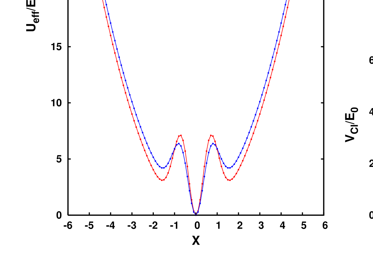
Figure 1: (color online) Plot of the effective time independent potential versus XX for very weak damping with external driving potential Ve​x​t(x,t)=Γexp(−x2/a2)cos(Ωt)V_{ext}(x,t)=\Gamma\exp(-x^{2}/a^{2})\cos(\Omega t) (a) without (red filled circle; V~0+V~c​l\tilde{V}_{0}+\tilde{V}_{cl}) and with (blue filled square; V~0+V~c​l+V~Q​D\tilde{V}_{0}+\tilde{V}_{cl}+\tilde{V}_{QD}) quantum dissipative part, (b) only quantum dissipative part (V~Q​D\tilde{V}_{QD}) and (c) only classical part (V~c​l\tilde{V}_{cl}). To plot this figure we used γ0/m​ω0=0.08\gamma_{0}/m\omega_{0}=0.08, Ω/ω0=150\Omega/\omega_{0}=150, A=17.85A=17.85, a/ℏm​ω0=0.71a/\sqrt{\frac{\hbar}{m\omega_{0}}}=0.71, and kB​T/ℏ​ω0=0.1k_{B}T/\hbar\omega_{0}=0.1. We have set ℏ=m=kB=1\hbar=m=k_{B}=1.

The above equations are expressed in terms of dimensionless variables X~=X/a\tilde{X}=X/a, A=Γ216​m​E0​Ω2​a2A=\frac{\Gamma^{2}}{16mE_{0}\Omega^{2}a^{2}}, and [⟨δ~​x^2⟩]0=[⟨δ​x^2⟩]0/a2[\langle\tilde{\delta}\hat{x}^{2}\rangle]_{0}=[\langle{\delta}\hat{x}^{2}\rangle]_{0}/a^{2}.

Refer to caption
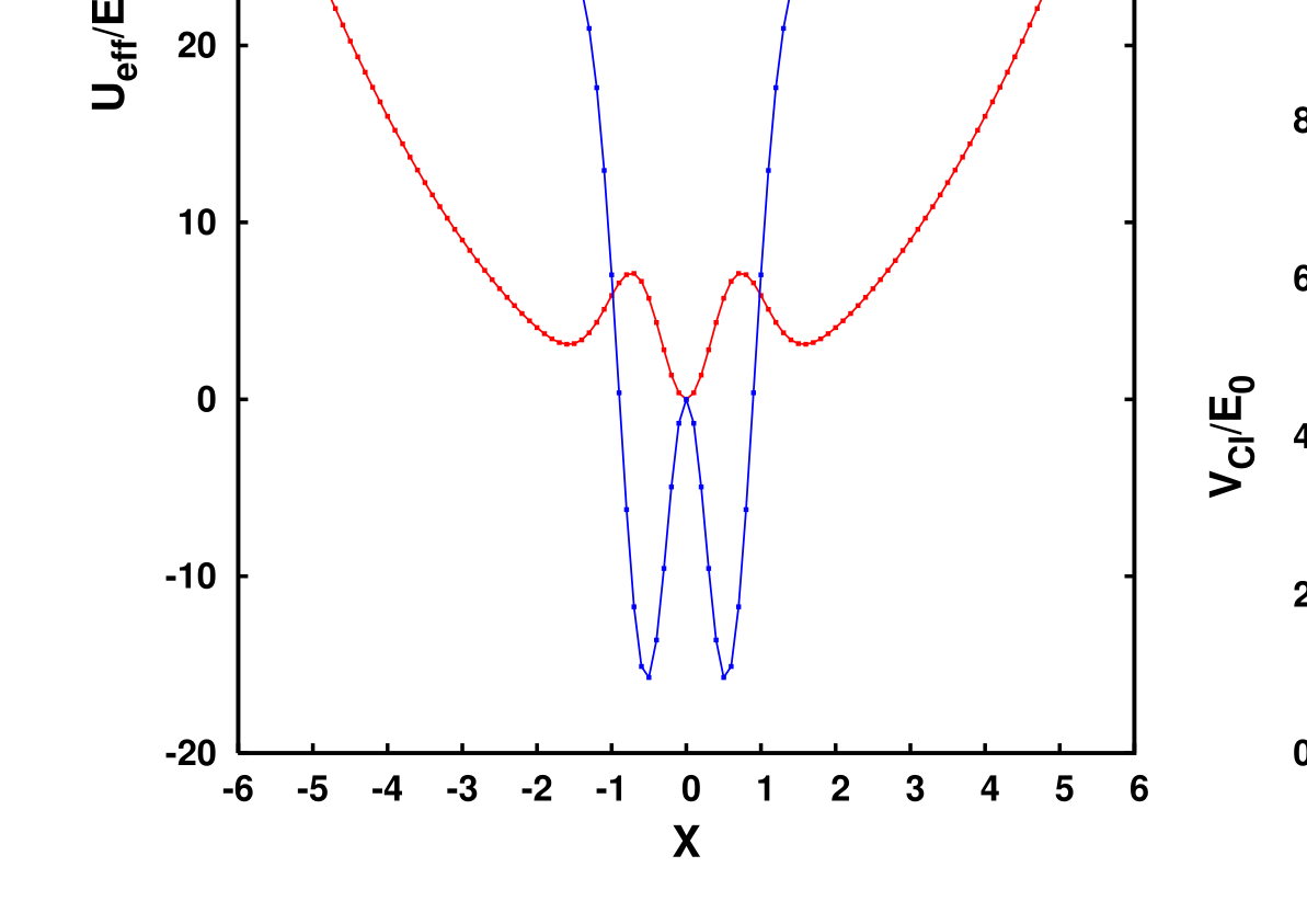
Figure 2: (color online) Plot of the effective time independent potential versus XX for moderate damping values with external driving and parameters as in Figure 1, except γ0/m​ω0=1.0\gamma_{0}/m\omega_{0}=1.0.
Refer to caption
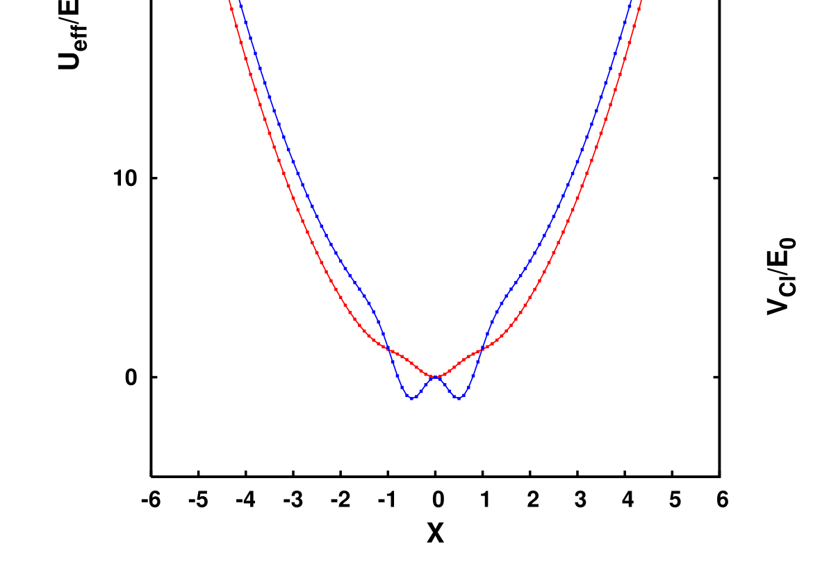
Figure 3: (color online) Plot of the effective time independent potential versus XX for high damping values with external driving and parameters as in Figure 1, except γ0/m​ω0=10.0\gamma_{0}/m\omega_{0}=10.0.

Figures (1), (2), and (3) depicts the effective potential profile in the low, intermediate and high damping cases respectively. As remarked in the previous paragraph, we see that the effects of VQ​DV_{QD} are most pronounced at intermediate values of the damping. The presence of higher order derivatives of space dependent terms of forcing in the quantum dissipative part, VQ​DV_{QD}, brings in some interesting changes in the qualitative form of the effective potential. It is evident from figure (1) that in the absence of dissipation the effective potential has two metastable minima and one stable minimum . But, on adding VQ​DV_{QD} two metastable states become stable minima and the stable minimum becomes a maximum.

5 Conclusion

In this paper, we have analyzed the properties of a quantum particle in a harmonic potential, coupled to a dissipative Ohmic heat bath, in the presence of a space dependent rapidly oscillating field. Starting from the usual heat-bath reservoir model, we obtained a cc-number GQLE from the operator equivalent by using a coherent state representation of bath oscillators [14, 15]. This enabled us to apply the Kapitza idea of separating into a slow part and a fast part, which consists of the rapid oscillations around the slow motion. The resulting equation for the slow motion is treated perturbatively. To leading order, we find that the rapid forcing leads to an effective static potential which has a quantum contribution, VQ​DV_{QD}, which adds to the classical result. This quantum contribution vanishes for both very small and very large values of the damping, but can have an appreciable and interesting effects for intermediate values. For instance, the number of stable minima in the effective potential can change, as illustrated by the case of a Gaussian oscillating force, for moderate values of the damping.

References

  • [1] W. Paul, Rev. Mod. Phys. 62, 531 (1990); W. Paul and M. Raether, Z. Phys. 140, 262 (1955).
  • [2] V. V. Balandin, M. D. Dyachkov, and E. N. Shapshnikova, Particle Accelerators 35, 1 (1991); R. Cappi, R. Gaoby, and E. N. Shapshnikova, CERN/PS 92-40 (RF) (1992).
  • [3] P. L. Kapitza, Zh. Eksp. Teor. Fiz. 21, 588 (1951); Collected Papers of Kapitza edited by D. Ter Haar (Pergamon Press, Oxford, 1965).
  • [4] L. D. Landau and E. M. Lifshitz, Mechanics (Pergamon, Oxford, 1960).
  • [5] I.C. Percival and D. Richards, Introduction to Dynamics (Cambridge University Press, London, 1982).
  • [6] S. B. Dutta and M. Barma, Phys. Rev. E 67, 061111 (2003).
  • [7] M. Bandyopadhyay, S. Dattagupta, and M. Sanyal, Phys. Rev. E 73, 051108 (2006).
  • [8] R. Zwanzig, J. Stat. Phys. 9, 215 (1973).
  • [9] G. W. Ford, M. Kac, and P. Mazur, J. Math. Phys. 6, 504 (1965).
  • [10] A. O. Caldeira, and A. J. Leggett, Ann. Phys. (N. Y.) 149, 374 (1983).
  • [11] U. Weiss, Quantum Dissipative Systems (World Scientific, 1993).
  • [12] R. J. Cook, D. G. Shankland, and A. L. Wells, Phys. Rev. A 31, 564 (1985).
  • [13] S. Rahav, I. Gilary and S. Fishman, Phys. Rev. Lett. 91, 110404 (2003); Phys. Rev. A 68, 013820 (2003).
  • [14] D. Banerjee, B. C. Bag, S. K. Banik, and D. S. Ray, Phys. Rev. E 65, 021109 (2002).
  • [15] D. Banerjee, B. C. Bag, S. K. Banik, and D. S. Ray, J. Chem. Phys. 120, 8960 (2004).
  • [16] M. Hillery, R. F. O’Connell, M. O. Scully, and E. P. Wigner, Phys. Rep. 106, 121 (1984).
  • [17] A. K. Pattanayak and W. C. Schieve, Phys. Rev. Lett. 72, 2855 (1994).
  • [18] A. K. Pattanayak and W. C. Schieve, Phys. Rev. E 50, 3601 (1994); and references therein.
  • [19] B. Sundaram, and P. W. Milonni, Phys. Rev. E 51, 1971 (1995).
  • [20] S. K. Sarkar and S. Dattagupta, Int. J. Mod. Phys. B 16, 1247 (2002).
  • [21] H. Grabert, Chemical Physics 322, 160 (2006).