SLAC-PUB-13425
SU-ITP-08/24
Simplified Models for a First Characterization of New Physics at the LHC
Abstract
Low-energy SUSY and several other theories that address the hierarchy problem predict pair-production at the LHC of particles with Standard Model quantum numbers that decay to jets, missing energy, and possibly leptons. If an excess of such events is seen in LHC data, a theoretical framework in which to describe it will be essential to constraining the structure of the new physics. We propose a basis of four deliberately simplified models, each specified by only 2-3 masses and 4-5 branching ratios, for use in a first characterization of data. Fits of these simplified models to the data furnish a quantitative presentation of the jet structure, electroweak decays, and heavy-flavor content of the data, independent of detector effects. These fits, together with plots comparing their predictions to distributions in data, can be used as targets for describing the data within any full theoretical model.
I Introduction
The LHC experiments are the largest and most complex in human history, with great potential to shed light on fundamental physics. As the experimental collaborations prepare to search for evidence of new physics at the TeV scale, particle physicists must also prepare for the next step: finding a framework in which to describe the data.
The Standard Model served this role through the entire history of hadron colliders, from the discoveries of the , , and top quarks through percent- and sub-percent-level measurement of their properties with Tevatron Run II data. But there are many proposed extensions of the Standard Model; many have qualitatively similar phenomenology, which depends dramatically on a large number of free parameters. Within the Minimal Supersymmetric Standard Model (MSSM), for example, each signature that is commonly searched for can be produced in multiple ways. When a signal is seen, it will not be immediately clear what particles are producing it, what their dominant decay modes are, or what other species are simultaneously produced. For this reason, it is useful to step back from the detailed predictions of any one model or region of parameter space, and characterize these basic properties first in a manner that allows comparison to any model.
In this paper, we propose a specific approach to characterizing the first robust evidence for new physics seen at the LHC. We present four “simplified models”, each with a small set of unambiguous parameters, based on the phenomenology typical of SUSY but stripped of much of the complexity possible in the full parameter space of supersymmetry. Despite their small size, these simplified models will give a good coarse-level description of SUSY-like physics, especially appropriate in the low luminosity limit. We discuss and illustrate by example how the parameters of the simplified models can be constrained, and how deviations from the simplified models in the data can be used to further characterize the underlying physics. We also discuss how to use these models as a basis for comparison of data with theoretical models such as the MSSM.
These simplified models are a useful first description for any “SUSY-like” new-physics signal in jets+MET+X. By this we mean that the new physics has a discrete spectrum of narrow resonances, that the new particles are odd under some exact parity and are “partners” of a Standard Model particle (with the same Standard Model gauge and flavor quantum numbers), and that the lightest parity-odd particle, which is necessarily stable, is neutral (and hence a dark matter candidate). These theories include not only the -parity conserving MSSM (see, e.g., [1]), but also UED models with conserved KK parity [2], Little Higgs with parity [3], and Randall-Sundrum models with custodial SU(2) and discrete symmetries [4].
The simplified models are expected to reproduce kinematics and multiplicities of observed particles remarkably well in a wide variety of SUSY-like new physics models — even when the spectrum of unstable particles in the full model is far more complex than the simplified model permits. The simplified model fits can then be used as a representation of the data, and can be compared to any full model by simulating both in a simple detector simulator. This last process of comparison can be done by phenomenologists outside the LHC collaborations.
The paper is organized as follows: In the rest of this introduction, we will motivate the approach of using “simplified models” to characterize data, and our particular choice of simplified models. We first consider alternative characterizations, and why we are led to the counterintuitive choice of trying to match data with models that we know to be incomplete (Section I.1). We then discuss which features we wish our approach to well describe, and define the simplified models (I.2).
In Section II we review basic features of SUSY-like phenomenology (II.1). This leads to a set of questions we can ask about any robust excess of new-physics events that is seen in jets and missing energy searches (II.2). This section can be skipped by the reader familiar with SUSY phenomenology. We give a detailed description of the four simplified models, and introduce variables that can be used to constrain their parameters, in Section III.
We present the first of two examples in Section IV. In this example, the simplified models describe the data very well, which allows us to use the results directly as a basis for model-building.
In many other cases, the structure of new physics breaks one or more of the assumptions in the simplified models. In this case, the “best fit” within the simplified models must be interpreted carefully. We discuss such subtleties in Section V. They also play an important role in our second example (Section VI). In this case the simplified models reproduce some features of the data, but not others, and we focus on how the simplified models can be used to test particular hypotheses for new physics.
I.1 Motivation for Simplified Models
If evidence for SUSY-like new physics is seen at the LHC, it will be presented and characterized in several ways. Both CMS and ATLAS are expected to present kinematic distributions, comparisons of data to SUSY benchmarks, and parameter fits within small parameter spaces such as the CMSSM and possibly larger ones. Why add another characterization to this list? Moreover, why characterize data in terms of deliberately incomplete models, when full models can be simulated quite accurately?
To address this question, we begin by summarizing the importance of comparing distributions in data to models, rather than presenting distributions alone. Some observables, such as the locations of kinematic features, can readily be read off plots. The analysis for producing such plots — jet energy scale correction, etc. — has become standard at CDF and D0. Properties that do not lead to sharp features are harder to determine. For example, counting events with different numbers of quarks from the frequency of -tags in data requires inverting differential tagging efficiency and mis-identification functions that depend on the kinematics of every jet in an event; to the authors’ knowledge this degree of “unfolding” based on data alone (not to be confused with measuring the rate of a process with a fixed number and distribution of -jets, e.g. ), has not been done in the past.
We encounter the same kind of difficulty in answering also much simpler questions: is a search that finds twice as many muon as electron events above expected backgrounds evidence for new physics that couples differently to electrons and muons? The answer depends on the differences in isolation requirements and detection efficiencies for the two flavors.
Both problems illustrate a key reason to study the consistency of data with models of new physics — the detector’s response to a model is subject to uncertainties, but is at least well-defined. A model that describes the data well is an invariant characterization of that data, independent of the detector. Finding such a characterization is the primary reason that comparing data to models, even at an early stage, is useful.
There is clearly a delicate balance between studying large and small parameter spaces: a small parameter space can be studied more efficiently and more thoroughly, but is less likely to contain a point that describes the data well than a larger space. Small subspaces such as mSUGRA (with four real parameters) are obtained by imposing relations between masses with little physical basis — for instance, a nearly fixed ratio of gaugino masses. The most dramatic changes in phenomenology typically arise from a re-ordering of the spectrum, which the mSUGRA mass relations prohibit. On the other hand, to cover all LHC phenomenology possible within the MSSM, one must scan over Lagrangian parameters.
The compromise — enlarging a parameter space until it can explain the data, but no further — is a natural one. It is likely that an MSSM point consistent with early new-physics data will be found in this manner, and it is a very useful result; what is unreasonable to expect is a thorough scan of the MSSM parameter space, in which each point is compared directly to data. Of course, this is even less probable where it concerns models beyond the MSSM. Therefore, we would like not only a consistent model, but an understanding of what structure is required for consistency (some subtleties of model discrimination at the LHC have been studied in [5] and [6]).
In answering this question, the simplified models, which have the simplest spectra compatible with SUSY-like structure, are an ideal starting point because they are — both practically and morally — minimal. They have few parameters not because of relations but because they contain only 2-4 new particles. Deviations from the phenomenology of the simplified models can be taken as evidence for a larger set of particles playing a role in new physics, and they are a natural starting point for building more accurate models.
Besides being a stepping stone to finding more accurate models, the simplified models work as baseline models to present in their own right. As we will illustrate in Sections IV-VI, they can describe many features of the data in a manner that is useful to further model-building, even when they do not reproduce all observables. This description motivates specific consistent models, which in turn suggest particular experimental tests to distinguish among them.
Finally, the simplified models suggest that imposing parameter relations is not the only way of reducing the SUSY parameter space, and may not be the most useful. As noted earlier, mass relations are particularly restrictive because they prevent interchanges of particle masses that qualitatively change phenomenology. By design, the simplified models have a small set of parameters whose variations have large effects on observables. These are the most important parameters to focus on in a first characterization of evidence for new physics. If technical obstacles permit detailed study of only a few-parameter space of models, the simplified models may be the most efficient alternative.
I.2 Introducing the Simplified Models
Two of the problems that motivate searching for TeV-scale physics — and that motivate a “SUSY-like” structure of Standard Model particle partners, among which the lightest is stable — are dark matter and the hierarchy problem. As we try to study the structure of physics at the LHC, it is useful to keep both in mind.
The lightest parity-odd particle (LSP) is stable, and a leading candidate for the dark matter in the universe. Being stable and invisible, it cannot be probed directly at a hadron collider, but its couplings can affect the decay chains of other, heavier particles. Within any model, such as the MSSM, the LSP can account for dark matter in some regions of parameter space but not others, and in some regions the standard cosmology is inconsistent with direct dark matter detection experiments. The decay modes of color-singlet particles offer one probe of what regions of parameter space we could be living in; these typically result in emission of weakly interacting Standard Model particles — , , and Higgs bosons, and/or pairs of flavor-correlated leptons or lepton/neutrino pairs. Characterizing the relative rates of these decays is thus a first step in relating TeV-scale physics discovered at the LHC to cosmology.
Natural solutions to the hierarchy problem also require relatively light partners of the top quark, and by association the bottom quark. The lack of discovery of such partners at LEP and the Tevatron already makes all known solutions to the hierarchy problem look a little fine-tuned, creating what has been called the “little hierarchy problem”. Confirming the presence of these partners confirms that the new physics solves the hierarchy problem; determining where they appear in relation to other new states sheds light on how natural the solution is. If these partners are produced, either directly or through decays of a gluon-partner, there will be an excess of and/or -rich events. Another feature that can give rise to extra or quarks is a light Higgs partner — this gives some hint at the structure of electroweak symmetry breaking.
With this in mind, there are three initial questions that can tell us a great deal about the structure of TeV-scale physics, and touch on questions of fundamental interest like dark matter and the electroweak hierarchy:
- 1. What colored particle(s) dominate production?
- 2. What color-singlet decay channels are present, and in what fractions?
- 3. How -rich are events?
The four simplified models proposed in this paper are designed to answer these questions. They are compact — 2-3 masses and 3-4 branching ratios and cross sections for each model — and retain a structure motivated by solutions of the hierarchy problem, but pared down to a parameter space that can be easily studied. This makes them ideal for experimental analyses with limited statistics and an excellent starting point for developing more refined theoretical frameworks to test against data. These simplified models are illustrated in Figure 1; we will specify them fully in Section III.
Lep(Q)


Lep(G)

Btag(Q)

Btag(G)

Each of the four simplified models includes direct production of only one type of strongly interacting species, either a quark or a gluon partner. The leptonic models Lep(Q) and Lep(G) are designed to parameterize the color-singlet particles produced in decays, question 2 above. The quark or gluon partner decays to one or two light quarks, plus either an LSP or an intermediate state that decays to the LSP by emitting a or boson, or a or pair. We will see that these two models typically provide a good description of new physics even when it contains multiple cascades, or multiple initial states. Associated production of quark and gluon partners when they have similar masses can be viewed as an interpolation between Lep(Q) and Lep(G).
The -tag models Btag(Q) and Btag(G) are designed to parameterize heavy-flavor production (question 3), as well as 1. By comparing data to these two models, one can quantitatively describe the rates of heavy flavor processes, and establish whether data is consistent with quark flavor universality, or whether the third generation is enhanced or suppressed. In the gluon partner model, Btag(G), the gluon partner decays to light quark pairs, pairs of -quarks or pairs of -quarks. In the quark partner model, Btag(Q), there are instead three different pair-produced species: light-flavor quark partners, -quark partners and -quark partners, which decay to their respective partner quarks.
Despite their simplicity, these four models can describe the kinematics and numbers of reconstructed physics objects remarkably well (including jets and either leptons or -tags, though not necessarily both leptons and -tags in the same model). Therefore, one may conclude that they also reproduce the properties of idealized physics objects, and the agreement is not sensitively dependent on details of the simulations. When this agreement is observed, the best-fit simplified models furnish a clear and simple representation of the data, which any physicist can compare to a full model by simulating both. This procedure should be valid, even when the simplified model-to-full model comparison is done with a simple parameterized detector simulator that has not been tuned to data. This application underscores that, though model-independent, the simplified models are most effectively used in conjunction with full models. Their virtue is that this characterization can be easily used with any model, because no correlations are imposed between different parameters.
II The Phenomenology of SUSY-like BSM Physics
In this section, we elaborate on what “SUSY-like” physics means, defining and discussing its important phenomenological features. In order to clearly understand how our simplified models are motivated theoretically, it will be useful to first consider the structure of the MSSM, highlighting its features at the level of quantum numbers and typical decay patterns. In the process, we will discuss non-MSSM (though still “SUSY-like”) physics using a more topology-based language.
Operationally, “SUSY-like” includes theories with new particles that carry Standard Model quantum numbers (partner particles) and a parity (under which partner particles are odd) that makes the lightest such partner particle stable. This in turn means that LHC processes are initiated by pair production. We begin by summarizing the particle content of different SUSY-like models. Within the MSSM, the particle content is fixed — two Higgs doublets complete the matter fields, and every Standard Model particle has partner with the opposite spin, but the same charges under . We expect all of these partners to have TeV-scale masses, and flavor-conserving decays.
Universal Extra Dimensions (UED) has an infinite tower of KK modes for each Standard Model state; if the theory is compactified on an interval, these KK towers alternate between parity-even and -odd states. UED is often considered as a “foil” for supersymmetry because the first set of KK modes, like SUSY partners, are parity-odd [2]. Little Higgs models have a smaller slate of partner particles — minimally, for the top and the gauge bosons [3]. Like UED, they also have parity-even new states. In this note, we focus on the phenomenology of the first KK level, or the T-parity-odd states in Little Higgs models, whose phenomenology is quite similar to that of supersymmetric partners.
The unique challenge of describing SUSY-like phenomenology comes from the sensitivity of both particle production and decay to particle masses. Typically, production is dominated by strongly interacting particles, i.e., in SUSY, either squarks or gluinos. The production cross-sections vary greatly as a function of mass — roughly as or faster as shown in Figure 2. Thus, depending on the squark and gluino masses, either gluino or squark production can have a much larger cross-section than the other, and the dominant production mode will change accordingly.


Similarly, a given particle’s decays depends sensitively on masses: if, as we assume here, there is a conserved parity under which “partner” particles are odd (or even if the parity is only approximate), every partner decays to a Standard Model particle and a partner. The couplings controlling these decays range from the hypercharge coupling to — the partial widths of different 2-body decay modes span 2-4 orders of magnitude (some also depend on mixing angles), so of all the kinematically allowed modes, those modes with the largest coupling constants dominate; however, re-arrangement of masses can forbid would-be dominant decay modes, so that small-coupling modes dominate. The range of partial widths is wider still for three-body decays.
The task of the rest of this section will be to map out the common topologies and decays that partner particle production can give rise to. We will focus on the MSSM, as it provides a complete set of partner particles, though other SUSY-like theories have very similar processes. Having done this, we’ll propose a set of questions that can guide the process of identifying what qualitative patterns of production and decay might exist in data. The goal of our simplified models will be to neatly encapsulate these patterns in a minimal way.
II.1 Typical Topologies for SUSY-Like New-Physics Production and Decay
We will find it useful to organize the production and decay modes according to the couplings of the particles: the production modes we focus on here are those with QCD couplings, which typically dominate at the LHC, so we will start from strongly interacting particles. Because partners are odd under a conserved parity, they decay through “cascades”, with one parity-odd particle and one or more parity-even particles produced at each stage of the decay. If possible, -charged states decay into other -charged states. once an -neutral state is reached, it is unlikely for decay to another -charged state to occur.
As a result, the R-parity conserving MSSM-like decay chains we are interested in here can be effectively divided into one -charged segment and one -neutral segment, in which decays are typically dominated by the electroweak interactions. Identifying the possible topologies for each stage allows us to ignore some ambiguities that will arise between, e.g., left vs. right-handed squarks and interchanges of the gaugino states (the “flipper” degeneracies of [5]), which are in general challenging to discriminate. This approach will suggest the simplifications we adopt in Section III.
In this paper we focus on phenomenology that can be described in the R-parity conserving MSSM with a heavy gravitino (this also includes, e.g., little Higgs and UED models with parities that have species with the same gauge and global quantum numbers but different spins), but does not describe models with light gravitinos or R-parity violation [1]. However, the classification we describe has a natural extension to these models, provided the additional interactions have small couplings to MSSM-like states, so that their main effect is on the decays of the LSP. In this case, we should add a 3rd “small-coupling” stage to every decay, after the “strong” and “electroweak” stages.
II.1.1 Production and Initial Decay of Colored Particles
Because they carry charges, squarks and/or gluinos will probably be the most abundantly produced new physics particles at the LHC. Depending on their masses, one or both will be readily produced. The associated mode () can also be competitive. Depending on their decay chains, the production of same-sign squarks from quark pdf’s (e.g. ) can be distinctive. Note that the associated and same-sign modes rely on quarks of the same flavor as the squarks that are produced — thus, they do not effectively produce third-generation squarks. Some estimate of the production cross-sections is given in Figure 2 (note that the cross-section depends not only on the masses of the produced particles, but on the masses of t-channel exchanged states as well).
The colored parts of decay chains, which typically end in a chargino or neutralino, are often quite simple:
Gluinos
can at tree level only decay through the interaction. When there are squarks lighter than the gluino, it will decay to these squarks (with relative rates determined by phase space), and not via off-shell states to three body; when the squarks are heavier, the gluino will decay through off-shell squarks to two quarks and a chargino or neutralino. In the latter case the branching ratios depend on the identities of neutralinos that are kinematically available, and the masses of the squarks. A simple parameterization is especially useful in that case. Note that, in either case, the decay is to two quarks of the same generation.
Squarks
can decay to a quark and a gaugino. When the gluino is lighter than a squark, decays to the gluino and a quark of the same flavor is often a preferred mode because it has the largest coupling. Other possible decays (and the only ones if the gluino is heavy) are to quark of the same flavor plus a wino, bino, or higgsino. When all of these are kinematically accessible, third-generation squarks will often favor the higgsino, left-handed squarks of the first two generation will favor the wino (third generation may be split between higgsino and wino), and right-handed squarks of the first two generations will go to the bino. Mixing among the gauginos can be important if they are light ( 300 GeV or less) and nearby in mass to one another, and this can slightly change these decay guidelines.
A squark always decays to an odd number of quarks, and a gluino to an even number. This can be useful, but there are kinematic regions where one of the emitted quarks is very soft (for example, a gluino decay to a nearly degenerate squark). In this case, it is possible to think of the gluino production as an additional contribution to the squark production cross-section, with an additional (softer) jet.
Note that three-body decay to a state with lepton number is in both cases suppressed, and is present only if none of the gauge or Higgs partners are available.
II.1.2 Electroweak Decay Chains
If the final decay product of the decay is the LSP, then there are no additional emissions; but when it is not the LSP, it decays down through one or more cascades from one electroweak-ino to another. These can be mediated by:
- •
Electroweak interactions of leptons, and/or Yukawa couplings of leptons — these lead to decays mediated by on- or off-shell sleptons, producing two leptons that may be charged or neutral. Different fractions of , , and can result from different hierarchies of masses and depending on whether the slepton is left- or right-handed: for example, decays through a right-handed slepton are often dominated by , while left-handed sleptons and sneutrinos mediate all three modes, often dominated by . The events are easily recognizable as an excess in opposite-sign leptons of the same flavor (“OSSF”) whose invariant mass does not reconstruct the mass. Moreover, these have a well-known characteristic invariant mass distribution, either an “edge” if the slepton is on-shell or an “endpoint” if it is off-shell.
- •
Higgsino-Higgs-gaugino interactions (SUSY partners of Higgs gauge couplings) allow decay through emission of a Higgs boson or (through the longitudinal mode) of the and gauge bosons. Off-shell , , and instead mediate a 3-body decay if the electroweak-ino mass splittings are too small for on-shell decays.
- •
gauge self-couplings allow emission of ’s, and in chargino-chargino decays, emission of bosons or (suppressed by ) photons. Again, the gauge bosons may mediate three-body decays if on-shell emissions are kinematically forbidden.
Note that all of these decays can occur irrespective of whether the initial and final electroweak-inos are bino-like, wino-like, or higgsino-like. The branching fractions are certainly sensitive to these changes, but the identification of partners is not sufficient to constrain these branching ratios. One reason is that decays through mixing can be competitive or even dominant, and the mixing matrix is extremely difficult to measure (knowing them requires measuring the masses and phases of all entries in the mass matrix, which most likely cannot be done at the LHC). The masses of sleptons and also play a significant role in determining the decay patterns.
A pragmatic treatment is to disregard the quantum numbers of the electroweak-inos, which are insufficient to determine branching fractions, and instead treat the unknown fractions as free parameters. We should then allow for direct decays of the -interacting sector into the LSP, and the cascades of heavier electroweak-inos to lighter ones as shown in Figure 3. If the bino, wino, and higgsino are all light (or just the wino and higgsino, with significant splitting between charginos and neutralinos), there can be multiple cascades, each stage with different branching fractions.

We have been deliberately unclear in Figure 3, in the case of charged emissions (e.g. ), about whether the decay is from a neutral state to a charged state, or a charged state to a neutral one. We do so because they might be difficult to distinguish In the former case, the light charged state must decay again to the LSP. However, if the state is a charged wino or higgsino in the same multiplet as the LSP, their mass splitting can be quite small ( GeV when ). The charged states decay to the nearly-degenerate LSP by emitting soft leptons or pions, which are difficult to measure, so the charge of this final state is lost.
We have assumed so far that decays of -neutral states to -charged states do not occur. Though they are impossible in CMSSM-like mass spectra, with winos and binos much lighter than the squarks, spectra for which these decays are permitted are logically consistent (for example, with a spectrum ordering ). Depending on mixing, the cascade can be possible. These additional jets are however typically significantly softer than the prompt jets from the directly produced state.
II.2 Eight Questions for the LHC
The phenomenology of SUSY-like models is quite rich, and the language presented above provides a useful framework in which to ask questions about data and build evidence for the answers. Many of the most interesting questions we would like to answer about the structure of new-physics production and decay processes are overly ambitious for a first characterization of data — they require a firm foundation as a starting point. The first goal is to build this foundation, by determining which of the processes discussed above are in play:
- 1.
-
Is production dominated by events with 2 hard partons (quark partners) or 4 (gluon partners)? As mentioned above, the physical interpretation is not always so simple — if the gluon partners are only slightly heavier than the quark partners, gluon partner production may dominate, but kinematically these events may look more like quark partner events. This may still be distinguishable from true quark partner pair production, either by the kinematics of softer jets or by the fraction of same-sign dilepton events. But in a first pass, these two alternatives are the ones to consider.
- 2.
-
What modes are present, and in what fractions? If pairs are seen, characterizing their kinematics (in particular, on- vs. off-shell sleptons and the implications of the edge or endpoint in their invariant mass for the mass spectrum). Decays to , and to pairs off the pole, are rather distinctive in dilepton invariant mass; more care is required in distinguishing bosons from pairs from sleptons.
- 3.
-
How -rich are events? The minimal interpretation of -rich events depends on whether we are dominated by quark or gluon partner production. If quark partners are light, the third-generation quark partners may well be even lighter — though they typically have smaller production cross-sections for the same mass, these modes are certainly worth looking for. On the other hand, three-body decays of a gluon partners can be approximately universal among flavors, or can be dominated by decays to the third generation — measuring these rates provides useful information.
These questions are well-posed within the simplified models we consider in this paper. But of course, they are only the beginning — to characterize the phenomenology, we must also consider correlations. In this paper, we will instead try to study these questions qualitatively using deviations of observed distributions from those predicted by our simplified models. Among these questions are:
- 4. Is there evidence for tops
-
(as opposed to independent production of ’s and quarks)?
- 5. Is there evidence for double cascades
-
from multiple electroweak-ino multiplets?
- 6. Are there differences in decays
-
between quark and gluon partners, between different quark partner species (e.g. left-and right-handed), or between heavy- and light-flavor decays?
- 7.
-
Is there evidence for competition between gluon and quark partner production modes?
- 8.
-
Are different tests of the features above consistent with one another? (for example: gluon partner pair production is expected to produce both a large number of jets and, if single-lepton decays are present, same-sign and opposite-sign dileptons in equal numbers).
Answering these questions gives insight into many of the most important properties of new physics that we can hope to establish at the LHC.
We should note that we are here deliberately leaving out questions concerning certain aspects of the new physics. Two omissions in particular deserve mention: spin determination and precision measurement of the new-physics spectrum. These questions have been extensively covered in the literature [10, 11, 12, 13, 14]. While these can, and should, be pursued in parallel with the questions we have emphasized, they often require correct assumptions about the mass hierarchy of partners and their decay topologies. Therefore the approach we are suggesting can be seen as a preparatory step for such further studies.
III Four Simplified Models
In this section, we present our proposal for how to characterize early excesses, keeping in mind the questions outlined above. We propose to use four simplified models, based on a number of well-justified approximations. Two models are aimed at capturing cascade decays that give rise to Standard Model leptons or gauge bosons, while two are aimed at describing the heavy flavor structure. We stress that each model is designed mainly to answer a targeted set of questions, not to necessarily provide a globally good description of data.
In these simplified models, we will assume that new-physics particle production is dominated by the pair-production of one new particle — either a gluon partner or a quark partner (where “a quark partner” indicates that we assume all prominently produced quark partners to have at least nearly degenerate masses, and that their properties can be characterized by averaging their decay branching ratios). This is a good approximation if mass scales for the gluon and quark partners the are widely split. If not, the resulting distributions will be a baseline of comparison for estimating the fractions of different production modes. The key reason for this assumption, however, is pragmatic: the clearest characterization of the data is found by comparing it to simple models, and this should come before any attempt to study more complex (and potentially more accurate) ones.
Our simplified models will only involve production of heavy particles, and we therefore expect that an On-Shell Effective Theory (OSET) approximation scheme is accurate [15]. In this scheme, matrix elements for production and decay can be approximated as constants (or with simple leading order corrections) and decays are described by pure phase space. With these approximations, the parameters of our simplified models will always take the form of cross sections for production, branching ratios for decays, and masses of on-shell particles (see Appendix A). We want to stress though, that this is only one way to simulate the processes, and while the simplified models can easily be constructed using a Lagrangian and implemented in a Matrix Element generator, the difference in the simulation is in practice negligible at the accuracy we target here.
III.1 Definition of the Simplified Models
III.1.1 Two Models for Leptonic Decays and Rates
We propose two models as a framework for studying electroweak cascade branching ratios in early data. The two models have identical decay structure, and differ only in that one is quark partner-initiated and the other gluon partner-initiated, which gives different jet structure of the decays. Each contains three mass scales: the primary produced particle or (quark partner or gluon partner), an intermediate electroweak state , and the lightest stable particle (LSP). The primary produced particle can decay either directly to the LSP, or to the intermediate state which then decays down by one of several channels:
- •
A boson (or off-shell with branching ratios if ).
- •
A boson (or off-shell with branching ratios if ).
- •
An pair, decaying through three-body phase space, unless there is kinematic evidence for an edge in the opposite sign-same flavor invariant mass, in which case it is replaced by a decay through an on-shell lepton partner.
- •
An pair, again decaying through three-body phase space, unless there is kinematic evidence for an edge in events, in which case the same on-shell lepton partner mass is used.
As we will argue, simplified models of this form are very effective for characterizing cascade decays involving Standard Model gauge bosons and leptons, even if when the underlying physics has a more complicated structure (multiple cascades, or multiple produced species with different decays).
The only “flat direction” in this choice of parameter space is the distinction between and decays. While this distinction is difficult to constrain (see sec. III.2.2 below), it is important to include to understand systematic effects on the fits (for example, the lepton or fractions, due to differences in signal efficiency, and the jet structure of the fits).
For quark partners, there is an ambiguity in the decay to the charged modes, and , between charge asymmetric and charge symmetric production. The former occurs when the intermediate color singlet state is charged, in which case up-type and anti-down type quark partners decays only to the positive intermediate state, and down-type and anti-up type quark partners decay only to the negative state. At the LHC, this means that production will dominate over final states. If the intermediate state is instead neutral while the LSP is in an SU(2) multiplet, as is the case, e.g., in anomaly mediation, the decay is flavor independent and charge symmetric (the remaining charge is then shed as soft pions or leptons when the charged SU(2) partner of the LSP decays to the neutral LSP). In order to avoid modeling different cross sections between and production, we choose the latter, charge-symmetric, decay mode for our simplified models. If data displays a difference between and production, this assumption can be modified as needed.
| Model | Particle content, SU(3)EM, mass | Rate parameters | |||||||||||||||||||||
|---|---|---|---|---|---|---|---|---|---|---|---|---|---|---|---|---|---|---|---|---|---|---|---|
| Lep(Q) |
|
| |||||||||||||||||||||
| Lep(G) |
|
|
The leptonic decay models are illustrated in Table 1, and in the upper panes of Fig. 1. The leptonic decay model for quark partner production, or Lep(Q) for short, has a total of 3 (or 4) mass parameters, , , (and if there is an edge in the dilepton mass spectrum), the most readily constrainable of which are the mass differences. There are 5 branching ratios (i.e. 4 unconstrained parameters), , , , and . Finally, there is 1 overall production cross section . Throughout most of this paper, we will just use the 7 (3 mass, 3 branching ratio, 1 cross section) parameter Lep(Q).
The leptonic decay model for gluon partner production, Lep(G), is identical to Lep(Q), except for the initial decay which is to two quarks. We use off-shell gluon partner decays, for two reasons. First, a series of two-body decays requires the quark partner to be lighter than the gluon partner; if it is not much lighter then the first decay will produce a rather soft quark, and will not look so different from direct quark partner production; while if it is significantly lighter, then direct quark partner production will dominate. Second, we want the two models to act as extremes for the jet structure of the decays, in order to “fence in” the underlying model; the greatest difference between quark partner and gluon partner decay is achieved with the gluon partner decaying to two jets of similar energy. Also Lep(G) has a total of 3-4 mass parameters (, , , and if needed ), 5 branching ratios , , , and (giving 4 unconstrained parameters), and 1 cross section .
Why do we suggest two models, rather than simply fit the number of quarks coming off the decay of the QCD particles to data? The reason is that fitting to the jet structure is in general quite difficult. Not only are jets complicated experimental object, jets are also abundantly produced in the underlying event and pileup at a hadron collider. While these effects can be subtracted, there are also many different sources for jets from the hard interaction itself: Initial state radiation jets, which depend on the masses of the produced particles; jets from the decay of the heavy QCD particles to color singlet states, with characteristics dependant on the different mass splittings present; and finally jets from the decay chains, in particular due to the presence of electroweak bosons and Higgs. This means that in order to get a fit right to the number of jets from the initial decay of the QCD particles, one must first model all the other aspects correctly. We therefore keep the description of the jet structure qualitative, and use different extreme choices to get a measure of which scenarios are more or less compatible with the data.
III.1.2 Two Models for B-tags and Rates
The b-tag models are constructed with the primary intention to quantify the heavy flavor quark fraction of the data, ignoring the lepton structure (which is studied using the leptonic decay models). This means that they are considerably simpler than the two leptonic models; in particular the presence of intermediate cascade decays is ignored. Differences in jet structure and kinematics are studied by varying the fraction of b quarks vs. top quarks in the decays.
The reason for this division between lepton and heavy flavor properties, is that there is no a priory reason to expect the same decays of light and heavy flavor quark partners. Any model that attempts to fit them both simultaneously therefore risks getting many parameters, thereby reintroducing possible flat parameter directions as well as unconstrained choices for the model structure. See sec. V.3 for a discussion of particular cases when combined fits might be feasible and useful in a second pass.
| Model | Particle content, SU(3)EM, mass | Rate parameters | |||||||||||||||
|---|---|---|---|---|---|---|---|---|---|---|---|---|---|---|---|---|---|
| Btag(Q) |
|
| |||||||||||||||
| Btag(G) |
|
|
The b-tag models are shown in Table 2, and the lower panes of Fig. 1. The b-tag model for quark partner production, Btag(Q), has a total of 2 mass parameters, and and 3 cross sections, , and . In the b-tag model for gluon partner production, or Btag(G), we assume that the gluon partners do not carry flavor, and so we use only one primary production mode with multiple decays. In its simplest form, Btag(G) has only a single light flavor mode along with a mode. It is often useful to include modes as well, especially if there is evidence for bosons from the leptonic fits, or heavy flavor-lepton correlations. Throughout most of this paper, Btag(G) will include a mode. In all, Btag(G) has 2 mass parameters, and , 3 branching ratios, , and , and 1 production cross section .
III.2 Observables for Constraining Simplified Model Parameters
In this section, we present a general discussion about how to fit the simplified models to experimental data. These methods will be used, and elaborated on, in Sections IV and VI.
The observables we discuss are very standard, and indeed among the simplest used in the literature. The minimality of the simplified models will, however, allow us to use these very simple observables to fully constrain their parameters in a transparent manner.
III.2.1 Mass Signatures
Scalar -type observables are common mass estimators for SUSY-like topologies. There are many conventions for the set of objects included in the sum; we will include up to four jets with the highest ’s, all leptons, and the missing energy. This “effective mass” is sensitive to the mass difference between the produced particle and the lightest stable particle (times a prefactor in the range ). The peak location depends on both the production matrix element and the decay chain undergone by the heavy particles. This will be seen in our examples, where the favored mass estimate differs from one simplified model to another.
Intermediate mass scales can be constrained by lepton kinematics, particularly by the dilepton invariant mass if a prominent dilepton mode exists. The dilepton invariant mass distribution will have either an edge discontinuity if the decay proceeds through an on-shell lepton partner , or endpoint if it is three-body, at
| (1) |
The distinction, which can be difficult to discern at low statistics, is whether the distribution in is discontinuous at , or falls continuously to zero at . Lepton distributions provide a second constraint on kinematics, necessary to fix two out of three masses that play a role in the on-shell decay (, , and ).
The constraints above always leave one mass unconstrained. Absolute mass scales can be determined from endpoints in observables such as [16, 17], or simultaneously using constraints from several decay chains (e.g. [18]). Initial-state QCD radiation may also be useful in measuring masses, or at least provide a strong cross-check [19]. These techniques however rely on knowledge about the decay chains of the produced particles.
For the early stage of analysis we consider, when decay chains are unknown, we take a more pragmatic approach — it is typically sufficient to present a fit at one mass for the LSP, and the lowest mass consistent with data is a good benchmark for this purpose. In addition, it is useful to vary the masses coarsely over the widest consistent range. For this purpose, rough upper and lower bounds on the mass can be obtained from the new-physics production cross-section; these are particularly useful for gluon partners, whose the cross section is dominantly determined by QCD couplings, the mass and spin of the produced particles, and parton luminocities.
III.2.2 Signatures for Leptonic Model Rates
With the masses in the models fixed, the canonical lepton counts are in principle sufficient for constraining the branching fractions of the different decay modes in the leptonic models (with the exception of the vs. boson fraction): counting dilepton “ candidate” events ( or pairs with dilepton invariant mass in a window around ), events with opposite-sign, same-flavor pairs of leptons that do not reconstruct near the mass, and single-lepton events, can be used to constrain the frequency of events with one , lepton partner dilepton cascades, and single-lepton cascades (from lepton partners or ), respectively. Single-lepton decays are also constrained by the frequency of events with opposite-flavor or same-sign dileptons, and (to a lesser degree, due to smaller event samples) the different decay fractions are constrained by 3- and 4-lepton events. The production cross section and branching fraction for direct decay to the LSP can be estimated from the total number of events passing the cuts.
In some cases, lepton kinematics may permit an empirical distinction between and lepton partner-mediated modes, but they are often quite kinematically similar. In this case, it is difficult to fix these two modes independently, and the strongest handle will be the jet structure of different types of events. In the interest of minimality, it is reasonable to expect presence of but not (from lepton partners) if evidence is seen for ’s, and but not if evidence is seen for from lepton partners (unless there are ’s from top decays). Another effect to which one may be sensitive, is an anti-correlation between jet multiplicity and lepton counts, in the case of a , which should be missing in the case of pure . In general, we suggest fitting to extremes (no /no direct decay and no respectively) as well as a free fit, to study the systematic effects related to this ambiguity. Since different jet cuts are typically used on the different lepton number signal regions, the relation of and events might affect the fits of other parameters, such as vs. , or the total cross section vs. , in particular for Lep(Q) fits (see the examples in sec. IV and VI).
III.2.3 Signatures for B-tag Model Fractions
The most important function of the b-tag models is to parameterize the heavy flavor fraction of the events, why the most important discriminator here is the frequency of events with different number of -tags.
If a sample has a large fraction of events with leptons, this is good evidence for the presence of leptonic or electroweak cascades, which are not present in the two -tag models. In this case, it is most reasonable to constrain heavy-flavor decay modes in a lepton-inclusive event selection, using the proportion of top quark events to study systematics, similarly to the comparisons between and decays for the leptonic models.
If, on the other hand, a sample has fewer leptons (and, in particular, if there is no evidence for or decay modes), it is quite interesting to see whether these can be explained entirely by and production processes, with no electroweak cascades. In that case, the top quark fraction can be fitted using the tag fractions in different lepton number signal regions.
In general, we suggest that the approximately “flat direction” corresponding to including only quarks or and quarks in the decays, should be investigated in a similar manner that the difference between and decays can be studied in the Lep(Q/G) models. By doing the fits with no and no decays, respectively, as well as allowing the ratio between them to float freely, it is possible to estimate the systematic uncertainty of the fits due to differences in jet and lepton structure, as well as investigate to which extent the leptons in the data can be described by top quarks only or if there are indications for cascade decays involving leptons.
III.3 Using the Simplified Model Fits
For a first characterization of the data, the results of fits of the simplified models can already by themselves answer many questions, and in particular contribute to the questions we laid out in sec. II.2. An example of a case when this is particularly true will be given in sec. IV below. However, this is not the only use of the simplified models. Another purpose is to give people outside an experimental collaboration a “target” to guide them in the attempts to explain the data, defined independently of the detector. A simplified model that is consistent with data (in some limited and well-defined sense), after the experimental collaborations’ best accounting for Standard Model backgrounds as well as effects like jet energy scale, -tag efficiencies, and electron reconstruction, is a target that physicists outside the collaboration can try to match, either analytically or with their own simulations.
A simplistic map from any model onto the simplified model space can be defined by averaging over the decay modes of different states, weighted by production cross-sections. The map is not one-to-one, but rather reflects the wide variety of models that may be consistent with data, until specifically optimized discriminating variables have been studied. Nonetheless, when a simplified model agrees very well with data (as in the example of Section IV), it is reasonable to look for full models of new physics that do have one production mode with the branching ratios found in the simplified models.
A more robust procedure for precise characterization is to generate Monte Carlo for the simplified models and compare it to other models; it is reasonable to expect that, where the simplified model is consistent with data and (in some simulation environment) with a proposed model, the model is also a reasonable hypothesis for the data. This procedure is is illustrated in detail in Example 2, see Sec. VI below. For this to be possible, it is of vital importance that also a set of diagnostics plots are published by the experiments, with the simplified model fits indicated. It should be noted that, when the simplified model does not reproduce all kinematics, the comparison in a different simulator may introduce systematic effects; optimizing the observables used in the fit to reduce dependence on detector modeling merits further study.
Once one or several models have been found which in this sense reproduce the data, theorists can focus on finding further predictions and discriminating observables due to the models, which can then be further analyzed by the experiments. The simplified models, together with comparison plots, would be an excellent starting point for this work.
IV Example 1: Simple New Physics
In most of their parameter space, complete models of new physics have more complex structure than the four deliberately simplified models we have suggested. Nevertheless, we will show in this and the next two sections how comparing data to the simplified models provides information about new physics beyond what one can conclude from published data alone.
The model we consider in this section is a limit of the MSSM that is well described by the simplified models (we will consider the opposite case — a model with far more structure than the simplified models — in Section VI). As our purpose is to treat the SUSY model as an unknown signal, we defer a summary of its physics to the end of Section IV.2.
We have separated the discussion into two parts: first, in Section IV.1, the “experimental” task of constraining parameters of the simplified models and comparing them to data, and second, in Section IV.2, the “theoretical” exercise of drawing conclusions about model parameters from these results. We will interpret the fits of simplified models to the data in the context of the MSSM, but there is nothing SUSY-specific about the exercise and it could be repeated for any of the “SUSY-like” models. We emphasize that the “theorist” need not have access to the raw data or to an accurate detector simulator, but only to experimental results of the kind presented in IV.1.
IV.1 Comparison of New-Physics Signal With Simplified Models
We have idealized the experimental problem in several ways. We work in six “signal regions”: five with exclusively 0, 1, 2, 3, or 4 or more leptons ( or ), and a sixth lepton-inclusive region used only in the heavy flavor studies. Each region has different requirements on jet ’s, , and missing energy (specified in Section B.1); these cuts have been chosen to mimic event selections for SUSY searches proposed by ATLAS or CMS in TDRs and notes. We have not included backgrounds in this study, but by design they are expected to be small and controllable in these signal regions, with the main effect of slightly increasing the uncertainty of the simplified model fits (examples of comparison plots including backgrounds will be given in Sec. VI.4. We have represented the detector by the parameterized simulation program PGS [20]. We expect the LHC experiments would use the full set of tools they have available — modeling of backgrounds validated on control regions, detailed detector simulation, and corrections applied to signal Monte Carlo where necessary — to make the fits that we propose. Likewise, the variables we use in this discussion are only representative; the most discriminating variables that can be reliably modeled should be used. The SUSY pseudo-data and all simplified models were generated using Pythia 6.404 [7], with the On-Shell Effective Theory implementation of simplified models as described in Appendix A.
In the discussion that follows, we will use four kinds of observables (also described in Section III.2) to find consistent simplified models:
- Lepton Counts
-
(the number of events in each signal region, the breakdown by sign and flavor in 2- and 3-lepton events, and identification of pairs reconstructing a ) constrain the total cross-section and branching fractions in each leptonic model, but do not distinguish ’s from an admixture of and direct LSP decay modes. Lepton counts can also be useful in comparing bottom to top quark modes in the b-tag models.
- Jet multiplicity and kinematics
-
constrain the ambiguous direction within either Lep(G) or Lep(Q) — distinguishing ’s and contributions — as it is sensitive to the hadronic fraction. The results are quite different between Lep(G) and Lep(Q), because they have different hadronic decays of the initial state. Jet-counting should be interpreted with care, especially if the qualitative differences between data and a simplified model vary depending on jet definitions. Correlations between lepton and jet multiplicities are more robust, but require more statistics.
- Overall kinematic distributions
-
such as and , as well as lepton kinematics can be used to constrain the masses of particles in each of the four simplified models.
- -tag Multiplicity
-
is used to determine the branching ratios in the Btag(Q/G) models, and tagged jet kinematics is a useful diagnostic.
We will start by looking at the Lep(G) model, as it turns out to give the best fit to the data, and dissect it in stages. We summarize the ranges of parameters we will consider in Section IV.1.1; sections IV.1.2-IV.1.4 each focus on constraints on Lep(G) parameters coming from a different set of observables. The observables used to constrain Lep(Q) are quite similar, and the Btag(G) model is significantly simpler than the leptonic models, so we treat these two more briefly in Sections IV.1.5 and IV.1.6 respectively, focusing on the notable features of these fits rather than the methodology.
In these studies, we wish to determine what regions of parameter space are most consistent with data and what inconsistencies cannot be removed by varying parameters of the simplified models — we are not simply interested in a single “best-fit” point in parameter space. The simplified models are small enough that the more ambitious goal is attainable. We minimize a defined over lepton count distributions, and quote best-fit cross-section and branching ratios (subject to a constraint that removes the ambiguity). We treat overall kinematics and jet counting more qualitatively — rather than fitting to these distributions, we illustrate how they are affected in different extreme parameter choices, and between the Lep(Q) and Lep(G) models. We use this hybrid approach because quoting a “best fit” with error bars is a clear presentation of the leptonic constraints, but is misleading in the latter two cases, where true uncertainties in simplified model parameters are likely to be dominated by detector and modeling systematics.
In plots in this and following sections, we include a lower pane showing the fraction of the simplified model curve divided by the pseudo-data, with the data error bars represented as grey bands, in order to facilitate comparison of models with data.
IV.1.1 Comparison of data to the Lep(G) Model: A First Look
We will illustrate the role of each discriminating variable by studying parameter points that are nearly consistent with data, excepting a single discrepant distribution. Table 3 summarizes the parameter values of interest. At each point, we have fixed either or (as motivated in Sec. IV.1.3), and other leptonic branching fractions are optimized using the leptonic ; we have also fixed because there is no evidence for a non-zero mode. The table is divided into decay mode variations (top), consistent kinematic variations (middle), and inconsistent kinematic variations (bottom). The first line, “Model A”, reproduces all distributions of interest quite well, as do C and D. Model A appears as a solid red line in every plot in the next three sections. The alternative models will be displayed as dashed or dotted lines.
| Leptonic Decay Models for Gluon Partners (Lep(G)) | |||||||||||
|---|---|---|---|---|---|---|---|---|---|---|---|
| Label | Description | //()/ | (pb) | Leptons | Jets | Kin. | |||||
| Decay mode variations with best-fit kinematics | |||||||||||
| A | 600/300/—/100 | 5.4 | 0.15 | 0.43 | 0.42 | — | — | + | + | + | |
| B | 650/300/—/100 | 5.3 | 0.16 | 0.19 | — | 0.65 | — | + | - | + | |
| Kinematic variations (including on-shell kinematics) with no ’s, best-fit rates | |||||||||||
| C | 750/500/—/300 | 5.3 | 0.15 | 0.47 | 0.38 | – | – | + | + | + | |
| D | (on-shell) | 600/300/200/100 | 5.3 | 0.14 | 0.43 | 0.43 | – | – | + | + | + |
| E | 700/300/—/100 | 4.7 | 0.16 | 0.41 | 0.43 | – | – | + | + | - | |
| F | 620/400/—/100 | 5.7 | 0.13 | 0.46 | 0.41 | – | – | + | + | - | |
| G | (on-shell) | 600/400/345/100 | 6.0 | 0.13 | 0.46 | 0.41 | – | – | + | + | - |
| H | (on-shell) | 600/300/250/100 | 5.3 | 0.15 | 0.41 | 0.44 | – | – | + | + | ? |
| I | 600/300/—/100 | 5.6 | 0.16 | 0.22 | – | 0.63 | — | + | - | ? | |
| stat. error | N/A | 0.2 | 0.01 | 0.03 | 0.06 | 0.08 | 0.04 | ||||
IV.1.2 Constrained Branching Fractions from Leptonic Counts
Aside from ’s, each of the four leptonic decay modes in the Lep(G) model (, , , and direct LSP decays) leads to a very different leptonic signature. For example, the only sources of events are events where one gluon partner emits and the other , and fakes from independently constrained processes. Therefore, lepton counts constrain these branching fractions well if we force the fraction to zero. As evidenced by the mass variations in the bottom half of Table 3, significant mass variations do not affect the results of these fits by more than . We can conclude rather robustly that the total cross-section is to 600 pb, the branching fraction is , and the fraction .
One would expect that these models remain consistent if we replace and direct LSP decays with ’s, which decay to one lepton 32% of the time, and hadronically (which, in lepton counts, looks like a direct LSP decay) 68% of the time. For instance, models A and B from Table 3 both reproduce lepton counts as shown in Figure 4.


The ratio of rates of slepton-mediated and events is a useful constraint on models of new physics, but the ambiguity prevents us from constraining it directly (depending on particle masses, the two leptonic modes may give rise to different lepton kinematics, but in this case they are quite similar). Instead, we will try to distinguish between hadronic ’s and direct decays.
IV.1.3 Jet Kinematics/Counts and the Ambiguity
From the discussion above, we expect lepton counts to be nearly invariant under shifts when they are compensated by
| (2) |
By inspecting the “no-W” fit parameters in Table 3, we see that, if we decrease while compensating by decreasing and , the first to reach zero is . So the most extreme cases we can consider while preserving our success in matching lepton counts with Model A are defined by fixing either or .
The best fits in each of the two extremes are shown in Figure 4. As shown in Figure 5, however, the mode produces too many jets. Before drawing strong conclusions from this observation, it is important to verify that the agreement of the model without ’s, and the disagreement of the model with a high fraction, are insensitive to the jet definition. If, as in this example, the qualitative conclusion is insensitive to detailed jet definitions, we can conclude that a gluon-initiated decay chain cannot have a large fraction of events coming from ’s.


IV.1.4 Mass Variations in Lep(G) Models
Kinematic distributions such as and the di-lepton invariant mass constrain mass splittings between new-physics particles. Roughly, is sensitive to changes in the top-to-bottom mass splitting (), such as between lines A and E in Table 3, while is sensitive to changes in the intermediate splitting (e.g. lines A and F). These variations are shown in Figure 6. In each case, we use the best-fit branching ratios and cross-section, with fixed.
As mentioned in Section III.2.1, one direction in mass space does not significantly affect these kinematic distributions — it corresponds approximately (but not exactly) to shifting the masses of all new particles by the same amount (e.g. compare lines A and C from Table 3, with and 750 respectively).


Given that the data has a significant branching fraction, and in fact is consistent with a slepton-mediated branching fraction as large as 45%, it is reasonable to ask whether the slepton could be on-shell (we would typically expect the 3-body decay to have a much smaller branching fraction). As shown in Figure 7, at an integrated luminosity of 500 both off- and on-shell kinematics are consistent with the data; for example is all kinematics well described by line D from Table 3. We are again sensitive to the intermediate masses, which must produce a kinematic edge at GeV and reproduce lepton ’s. These constrain, for example, lines G and H of Table 3.


It is worth noting that kinematic distributions such as depend on branching fractions of the parent particle. For instance, if we substitute ’s for some of the fraction of best-fit model A, as in the second line of Table 3, the peak of the distribution shifts downward (see Model I, the green dashed line on the left panel Figure 8). To compensate for this, we must raise , as was done in model B in Table 3 (see right panel of Figure 8). A weakly constrained gives rise to a systematic uncertainty in the mass of the gluon partner within the Lep(G) model (more precisely, this is an uncertainty in the mass difference between the color octet and invisible LSP).


IV.1.5 Comparison of Lep(Q) Models
Constraints on the Lep(Q) models are quite similar to those discussed above. Again, we can reproduce lepton counts and event kinematics for suitable mass choices, with or without decays, as shown in Figure 9 (the model parameters used are summarized in Table 4). The jet structure, however, is inconsistent with production dominated by quark partners, for both extreme cases, as illustrated by Figure 10. The discrepancy is most clearly seen in the 2-lepton region, which even in the -rich scenario has few hadronic ’s.


| Leptonic Decay Models for Quark Partners (Lep(Q)) | |||||||||||
| Label | Description | // | (pb) | Leptons | Jets | Kin. | |||||
| Rate variations with uniform kinematics | |||||||||||
| A | 500/300/100 | 10.7 | 0.064 | 0.40 | 0.54 | — | — | + | - | + | |
| B | 600/300/100 | 6.1 | 0.11 | 0.19 | — | 0.69 | — | + | - | + | |
| Approx. error | N/A | 0.1 | 0.005 | 0.01 | 0.04 | 0.05 | 0.02 | ||||


IV.1.6 Comparison of Btag(G) Models
In studying heavy flavors, we will focus on Btag(G), which reproduces the jet multiplicities in the sample far more accurately than Btag(Q). Two lines of questioning are assisted by a comparison of the data to Btag(G) models: what is the heavy flavor fraction in decays, and can all the leptons be accounted for by ’s from top quarks (i.e., is the data consistent with a model with no electroweak cascades, even though there are leptons)? The second question is less relevant here because we already have strong evidence for electroweak cascades (the edge) and a strong argument that not all leptons come from ’s (from the Lep(G) analysis in Section IV.1.3).
Therefore, we include only the and modes in Btag(G), omitting the mode, and we tune the parameters by fitting to b-tag multiplicities in the lepton-inclusive multi-jet region (see Appendix B.1). Figure 11 shows the best-fit to -tag multiplicity and some tagged jet kinematics, for the best-fit choice in Table 5.
| B-tag Model for Gluino Partners (Btag(G)) | |||||
|---|---|---|---|---|---|
| Parameter | , GeV | , GeV | (pb) | ||
| Value | 600 | 100 | 4.0 | 0.84 | 0.16 |
| Approx. error | — | 0.2 | 0.03 | 0.03 | |


The agreement of our model with all multiplicities of -tags supports the two simplifying assumptions in the Btag(G) model: that there is only one initial state (or all initial states decay to jets in the same fraction), and that heavy-flavored jets are produced in pairs. The kinematics of these -jets is consistent with the expectation for , and favors this over production through top or Higgs decays (which were not included in the model, but are expected to produce softer jets).
The fit fraction consistent with heavy flavor is suggestive of nearly universal decays to 5 generations, with top quarks suppressed (perhaps by phase space). This leads us to ask: are the leptonic cascades in gluino decay independent of quark flavor? This question is beyond the reach of the simplified models, but is simple to study qualitatively, by comparing the -tag multiplicities in different exclusive regions — as shown in Figure 12, there is no obvious correlation.

IV.2 Interpreting the Simplified Model Comparisons
IV.2.1 Summary of Conclusions from Plots and Simplified Models
We begin by summarizing what is known (and suspected) about the model. Some of what we know can be inferred from plots alone:
- •
There is an on- or off-shell dilepton cascade with appreciable rate, with known edge/endpoint location
- •
There is evidence for events with no leptons, and for a prominent decay mode involving one lepton.
- •
There are -tagged events; by a ball-park estimate that 1/6 as many events have 1 tag as 0 tags; assuming a -tag efficiency of 30-50%, the average number of -jets per event is .
- •
There is no significant correlation between b-tag and lepton multiplicities.
The simplified model comparisons have given us more quantitative results, as well as information from jet modeling that could not have been derived by simply looking at plots:
- •
Jet structure is quite consistent for the leptonic decay model for gluon-partners, Lep(G), provided the hadronic / fractions are small. The leptonic model for quark-partner decay, Lep(Q), is inconsistent with observed jet multiplicities.
- •
The dilepton branching fraction is , and the combined single-lepton branching fraction (accounting for both slepton-mediated decays and leptonic ’s) is . Most of the remaining decays do not emit more jets with GeV (to a good approximation they are invisible).
- •
The heavy flavor fractions are consistent with pair production of a single particle that decays to light quarks 80-85% of the time and to heavy quarks , , or 15-20% of the time. The -tagged jet kinematics is consistent with direct emission, and probably not consistent with a dominant mode, or with emission from a Higgs in a cascade.
We now see what we can deduce about the underlying physics; in this section we will focus on analytical estimates within the MSSM; for example 2, in Section VI.4, we will use a more quantitative method, namely numerically simulating models and comparing them to simulations of the simplified models. For definiteness, in both cases, we will take the position of a theorist trying to explain the excesses seen at the LHC in the context of a SUSY model within the MSSM.
IV.2.2 Discussion: Consistent MSSM Parameter Space
As jet multiplicities are quite consistent with a four-parton topology, we will assume that the signal is dominated by gluino pair-production. There is a variation to keep in mind: squarks that are slightly heavier than the gluinos (and decay to them) may also be produced, but the additional jets may be fairly soft.
What is the origin for the decays? The study of rates in the Lep(G) model showed that they cannot all consistently result from ’s, if (as in the leptonic models Lep(Q/G)) at most one is produced in each cascade. Jet counts disfavor a significant mode, and would disfavor multi- cascades even more. So to explain the high rate of leptons in the signal, we assume that a large fraction come from a slepton-mediated mode. We have not obtained a lower bound on the fraction of coming from sleptons, but the good agreement with jet multiplicities in the limit leads us to ask what new-physics scenarios could be consistent with as in the Lep(G) model point A.
This suggests a roughly four-to-one ratio between and , which is rather striking. The ratio can be achieved in several ways for off-shell sleptons, but with a mass splitting GeV it is difficult to engineer couplings such that three-body decays dominate over and emissions. With on-shell sleptons, it is difficult to account for such a ratio. If the LSP is an singlet with no charged partner, and a mode is also open, then charged intermediate particles always decay to , while neutral intermediate particles may be evenly split between and modes. If charged and neutral parents are produced in equal rates, this gives one factor of two. For another factor of two, we must produce more charged than neutral states. This is achieved in gluino decays through off-shell squarks, where two modes for gluino decays to interfere constructively. This is also consistent with our results based on jet multiplicities in Lep(G) and Lep(Q), and it has significant implications for the spectrum. Firstly, in the MSSM, the LSP must be a bino and the NLSP either wino or higgsino. Secondly, the right-handed sleptons must be too heavy to play a large role in decays.
From Btag(G) comparisons, we learn that the fraction is consistent with a single production mode, that produces pairs of the time. A higgsino NLSP is implausible for two reasons: it would probably enhance the heavy flavor fraction well above flavor-universal rates, and would introduce an anti-correlation between leptonic decays and -tag multiplicity (decays involving light flavors would go dominantly to the bino LSP, without a cascade) which we did not observe. With a wino NLSP, this rate is likely consistent with universal squark masses, with decays suppressed by phase space.
We are fortunate, in this case, to be led to a unique ordering of relevant weakly interacting species, fully determined by the cascade and fractions we have measured (it is only unique if we take all the hints from the data seriously, such as the 45% branching fraction to , though it was only loosely constrained). These conclusions are indeed correct. The spectrum of the model is shown schematically in Figure 13 (the full Pythia parameter set is in Appendix B.3.1).

This “back-of-the-envelope model-building” is sufficient here only because the underlying new physics is almost as simple as the simplified models we have compared it to, but illustrates that constraints on the simplified models translate into quite strong constraints on new physics, and the model-independent statement of this constraint makes it easily usable in the context of any SUSY-like model. In Section VI, we will see specifically how the simplified models can be used even when the true structure of the new physics is significantly more complex.
V Probing Physics Beyond the Simplified Models
The simplified models have a rigid minimal structure, with only one pair-produced species and a limited set of one-stage electroweak decay chains. The kinematics of decay products in all modes are determined by uniform initial and intermediate particle masses; the pair-production assumption also leads to a specific “quadratic” correlation between the rates of different processes. These simplifications of both kinematic shapes and rates make the simplified models quite easy to constrain, but restricted. If new physics has a more complex structure, either kinematic shapes or rates may differ from simplified model predictions; these deviations suggest what additional structure is necessary to explain data.
In this section and the case-study of Section VI, we study several limits of new physics with structure beyond the simplified models. In these examples, deviations of observables from the simplified model predictions are quite statistically significant, but still smaller than one might expect. Indeed, the degree of success of simplified models in these cases suggests that more complex models needed to capture their structure would have very poorly constrained parameters. This justifies studying and presenting best-fit simplified models carefully even when they do not fully reproduce data, as a well-constrained coarse-grained description of tne new physics, in addition to seeking extensions consistent with all data.
We focus here on two of the most generic deviations in a SUSY context: multiple production modes, and particles that decay through a series of cascades. In the first case, the rapid fall-off of production cross-sections with particle mass (see Figure 2) simplifies the situation dramatically: because particles of much higher mass than the lightest produced particle (those that affect shape most significantly, leading, for instance, to a visible bump in ) are strongly suppressed. These rare production modes do not change rates enough to make the non-quadratic structure apparent. In the opposite situation, when multiple particles of comparable mass are produced, the effects on rates can be significant, as discussed in Sec. V.1 below. Fortunately, multiple production modes near the same mass scale are benign where it concerns shapes. When different jet production modes originate from a similar mass scale, the simplified models can match the broad kinematic structure of the trigger jets with just an overall and intermediate mass scale. So long as the gross structure of the jet counts are matched, which they usually are within the range of topologies in the simplified models, the qualitative shapes of jet and lepton structures in the data can be matched. Therefore, multiple production modes can significantly affect either rates or kinematic shapes, but not both.
The second effect, the presence of double lepton cascades, can have an impact on both rates and shapes, if the two chained decays have very different kinematics. Here, shape corrections are particularly easy to diagnose, as they can be seen in leptons (see the example in Section VI), though the inability to model these shape discrepancies in jets may be a concern. We have found in a large number of examples that the best fit to rates within the simplified models is remarkably good. The example of Section V.2 is representative.
A first characterization of data need not account for all correlations in multiplicities or kinematics of final state objects. However, when the correlation is large, it is desirable to describe it quantitatively. This can be done either by finding a consistent point in e.g. MSSM parameter space or by extending the simplified models to a larger on-shell effective theory (OSET)[15]. It is ideal to do both, with the MSSM point providing proof of concept and the larger OSET describing the consistent range of phenomenology in a model-independent way. In the latter case, the appropriate generalization of the simplified models depends on observations, and is beyond the scope of this paper, but we discuss one case of particular interest — correlations between lepton multiplicity and -counts — in Section V.3.
It should be emphasized that the basic count, object , and distributions are not the most sensitive means of finding deviations from the simplified models. But they are the distributions that govern modeling of detector response to objects in an event. Therefore, in order for any model to provide a meaningful approximation to the underlying physics, and signatures on the objects that are triggered on must be described well. Having done this, the approximate description can be used as a target for vetting models without having to worry significantly about systematic errors introduced by trigger rate mis-modeling. So the figure of merit for determining if the simplified models are good enough for approximating complex physics is how well , and very basic count observables are modeled. A very simple model that passes this test can be used for meaningful initial comparisons to other models.
V.1 Left/Right or Isospin Differences and Lep(Q)
The first deviation we consider is very generic when light quark partners dominate new-physics production: whereas the Lep(Q) simplified model contains one triplet, in SUSY we expect two new triplet scalars for each of the six flavors of quarks! Disregarding the third generation, we can expect approximate flavor universality across the first two generations, but decays of , and can be quite different from one another (a related complication occurs when both quark and gluon partners are produced, and favor very different decay modes). An extreme example is the case when the bino is the LSP and the winos have masses between the bino and the squarks, while the higgsinos are heavier than the squarks. The left-handed squarks couple dominantly to the winos, and therefore cascade decay emitting or lepton pairs/lepton + neutrino, while the right-handed squarks only decay directly to the LSP. Depending on the squark and gluino masses, the left- and right-handed squarks can be produced together or predominantly in pairs of particle-antiparticle. The assumption in Lep(Q), that there is only one particle species produced with a set of branching ratios to leptons and weak bosons, can give a better or worse description of the data depending on the mix of production processes.
The particular way in which the description fails gives important hints as to how the model can be amended. If in particular the associated production is absent, we would see an excess of different-flavor and same-sign two-lepton events as compared to single-lepton events, and vice versa if associated production dominates. Reliably modeling the actual mix of production modes, as well as the branching ratios and decay modes of the different species produced requires constraining at least 11 parameters (three cross-sections for pair production of two types of quark-partner and their associated production, and four free branching fractions for each species of quark partner). Without large statistics, the risk of having fits pulled by statistical fluctuations is also large once an increased number of parameters is introduced. Moreover, the interpretation of these effects is ambiguous, as similar features could instead point towards multiple-stage decay chains as discussed in the next section. We therefore recommend using such features in the fits of the model to early data as hints, and publishing the relevant comparison plots and pulls, rather than try to publish less stable fits with an enlarged parameter space.
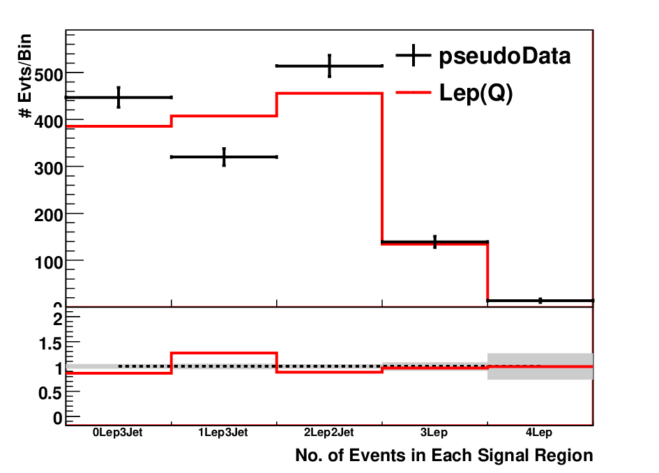

An example of diagnostics plots for the case outlined above, with decaying to lepton + neutrino or lepton pairs through intermediate winos, and only decaying directly to the LSP, is shown in fig. 14, together with the best-fit Lep(Q). The best fit balances the lack of different-flavor events in the two-lepton region with an overpopulated one-lepton region. The deficit of different-flavor events can be seen in the OSOF bin in the 2-lepton signal region lepton counts. Pseudo-data and Lep(Q) fit parameters can be found in Appendix B.3.4.
It should be noted that, in the early running of the LHC, before tau tagging is fully functional, a similar effect might be due to an over-representation of tau lepton decays. It is fairly generic to have tau lepton partners lighter than the electron and muon lepton partners. In this case, gauge boson partner decay into tau leptons will be enhanced with respect to light-flavor leptons, especially if the tau lepton partners are the only ones kinematically accessible below the gauge boson partners. Before the hadronic taus from these decays can be reliably tagged, only the leptonic tau decay will be noticed, leading to an enhancement in different-flavor leptons (and corresponding depletion of same-flavor pairs) with respect to the assumption of (most of) the light-flavor leptons coming from decay through light-flavor lepton partners. This situation will immediately be resolved once the rate of hadronic taus can be reliably estimated.
V.2 Multiple Intermediate-State Masses and Chained Cascades


Another effect that we have so far omitted from the discussion is the possibility of cascades chained one after the other (up to two within the MSSM, or more if higgsinos or winos have large splittings). The effects of a double cascade can be partially modeled by simply increasing the rates for cascade modes in a single-cascade model like Lep(Q/G). This will suffice so long as branching fractions are not required to obtain the observed frequencies of leptonic events.
The success of describing long cascades by these “flattened” models relies on low leptonic branching fractions of and bosons, such that — in early data — the statistical uncertainties in the rate of many-lepton events are likely to be quite large. So any optimized fit will be pulled most by the bins that are populated by only one leptonic decay. However, chained cascades that produce more weak gauge bosons have enhanced rates for multiple bosons to decay leptonically (because combinatoric factors are higher than for bosons produced singly). So chained cascades should first appear as excesses in multi-lepton events over what is expected from the rate of events with fewer leptons.
V.3 Lepton and Heavy Flavor Correlations and Extensions of the Simplified Models
In our simplified models, we chose to model lepton and heavy flavor observables separately, in order to keep the number of parameters down. The reason for this is that the number of extensions of the simplified models necessary to account for possible combinations is, even in just the MSSM, too large to be tractable. Furthermore such models would in general have too many parameters to be uniquely constrained by early data, which reintroduces flat directions and arbitrary fits. There are however certain situations where conclusions about lepton and heavy flavor correlations can be drawn from very simple extensions or combinations of the simplified models.
One such case, which can be seen directly from the simplified models, is when all leptons come from top decays. In this case, the Btag(Q/G) models including top decays will by themselves properly model all the lepton counts and kinematics. Such a case will be indicated in the Lep(Q/G) by an absence of modes (or s), and a jet structure compatible with decays rather than .
A second case is exemplified in Sec. IV. Here, we find that the Btag(G) fit is consistent with flavor-independent decay of gluon partners (with top decays suppressed by kinematics). In such a case, it is very natural to include decay modes, with branching ratios for the color singlets constrained to be identical to those in the decay to light flavor quarks.
If, alternatively, the Btag(Q/G) fits show that lepton and jet kinematics (such as invariant masses) are well described by the top hypothesis, but top quarks by themselves fail to explain all leptons in the data, another simple extension would be to add a direct top quark decay ( or production with ) to the Lep(G/Q) models.
Each of these extensions only introduce one extra parameter to the Lep(Q/G) models, describing the - or -rate, respectively. They can be used in a similar way as the four basic simplified models, to investigate to which extent data can be described, except that the relevant data now is correlations between leptons and -tags, such as the lepton counts for different number of -tags. Deviations from the expected fits can then be a basis for further conclusions about the spectrum and couplings. It is important, however, not to add progressively more complexity to account for every feature of observed deviations, since the uniqueness of descriptions of features then soon will be lost. It is also very important not to create extensions to model deviations that are not statistically significant. We therefore recommend, once again, to publish fits to the unextended simplified models alongside any extensions, the ones suggested here or others.
VI Example 2: Complex New Physics
Having considered a relatively simple example in section 4 to illustrate how simplified models can characterize and then represent the data, we now move on to a more intricate example. As pointed out in section 5, the allowed new-particle spectra — and hence the allowed decays — in “SUSY-like” physics can be much more complex than those of the simplified models. In section 5, we discussed common ways in which our simplifications can have an impact on the fits of the simplified models to data. We also commented on signatures that can be helpful for detecting what simplifications are violated by the underlying model, though we don’t expect that process to be very straightforward at low luminosity.
Here, we will consider an example where the underlying model is significantly more complicated than the simplified models. We will see that most basic signatures are well modeled by many limits of the simplified models. There are some sources of tension, mainly kinematical. While we won’t be able to clearly diagnose what’s different between the underlying model and each of the simplified models, we will be able to draw qualitative and quantitative conclusions about the structure of production and decay that will offer an excellent starting point for model building. We will highlight those aspects that cannot be simply read directly off plots of data alone, and illustrate the procedure of vetting more detailed model hypotheses against fits to the four simplified models, Lep(Q/G) and Btag(Q/G).
We will consider the SUSY model generated using the Pythia parameters of Appendix B.3.2 in Pythia 6.404 [7]. As before, the parameters are provided for reference, but we will treat this as an unknown signal for the remainder of this section. We also use the same set of “signal regions”, as described in Appendix B.1, that we used in Section IV.
In the following subsection, we provide a summary of the simplified model fits and main areas of agreement and tension with the data. We will discuss the Lep(Q/G) fits in detail in subsection VI.2 and the Btag(Q/G) fits in VI.3. In subsection VI.4, we will investigate how to use the simplified models for interpreting data.
VI.1 Summary of Model-Independent Results
In summarizing the main results of the simplified model fits, we will choose particular masses. We will not discuss the question of mass estimation in any detail for this example, as the emphasis is on how to use the fits. We have set the LSP mass to GeV, and then estimated the remaining mass parameters using , jet , and lepton . In table 6, we summarize fits to on- and off-shell leptonic models Lep(Q/G). Likewise, table 7 presents fits to the -tag-study models Btag(Q/G).
We now highlight features of the data evident from studying plots, and the refinements that are made possible by quantitative comparison to the simplified models. As they are closely related, we will list them together, with the conclusions from distributions alone in italics:
- •
Gluon or quark partner models alone do not give a good description of the jet structure, suggesting that a combination of production modes is required. Fits to the total event rates suggest a cross section in the range of pb. A lower bound estimate of the mass scales is, GeV, with GeV. Referring to figure 2, this strongly supports the hypothesis of production of particles charged under SU(3).
- •
There is an OSSF dilepton decay mode. We can conclude this from the excess of OSSF events over OSOF (and other dilepton events). There is also a di-lepton invariant mass structure that suggests either on- or off- shell lepton partners.
- –
From the leptonic simplified model comparisons, we conclude that an decay mode occurs in of decay chains.
- –
There is also strong evidence for a sizable channel, with branching fraction .
- –
The observed fraction appears small, in the range of .
- –
It is difficult to obtain enough opposite flavor di-lepton events without overpopulating single lepton events. In addition, the shape of the lepton signatures, as compared to the fits to Lep(Q/G), suggests that there is a missing source of relatively soft leptons. The data must include some source of leptons not included in the simplified models.
- –
- •
There is a preponderance of -jets, with extremely high tag rates. We learn significantly more detail from the fits to Btag(Q/G) simplified models:
- –
The distribution of -jet counts is pretty well accounted for by pair production of a gluon partner that decays to a pair of 3rd generation quarks of the time, and a pair of light-flavor quarks the remaining of the time.
- –
When the heavy-flavor decays are all to , we correctly reproduce both -jet distributions and the lepton/b-count correlations in events with more than one -tag.
- –
There is slight disagreement between the -tag multiplicity predicted by Btag(G) and the data — in particular, we cannot account for all the 1- and 2-tag events without over-estimating the number of 3- and 4-tag events. This is only an effect at the statistics shown. If we take it at face value, the simplest interpretation is that there is a distinct production process that produces up to two heavy flavor quarks (for example, either stop or sbottom production or associated production of the gluon partner with a light-flavor quark partner.
- –
- •
There is a qualitative trend in the -count distributions as we move across lepton regions: the lepton-rich events have fewer -jets. From the quantitative comparison to Btag(G), we saw also that the difference is approximately compatible with adding sources of leptons to zero- events. This gives evidence that the mode appears dominantly in light-flavor decays (either of the gluon partner or of some other state). Using the light-flavor fraction from the Btag(G) fit, we are led to hypothesize an decay mode in of these light-flavor decays. This number was inferred indirectly and should not be trusted too much.
- •
The jet multiplicity in 2-lepton events seems significantly lower than in 0- or 1-lepton events — but there are many interpretations: A decrease in lepton ID efficiency in events with many jets? ’s that produce more jets when they don’t decay leptonically? Or evidence that 2-lepton events are dominated by a mode with fewer partons from the decay? The approximate consistency of Lep(G) (with ’s) with the jet counts shown in Figure 16 suggest that ID efficiencies and decays are sufficient to explain this trend. Other interpretations are also possible (these jets could be radiation, or products of heavier states decaying to gluon-partners).
Some other features are beyond the resolution of the simplified models — for example, we can’t repeat the fit to leptonic branching fractions in the presence of a top-quark decay mode. We have, however, built evidence for the basic structural components of the new physics, and found a characterization of the new physics to which we can compare any model.
In the following sections, we discuss in more detail the structure of the Lep(Q/G) and Btag(Q/G) characterization of the data. However, the above summary is sufficient for discussing how to use the fits presented in tables 6 and 7. We therefore recommend that the reader interested in this topic skip to subsection VI.4.
VI.2 Comparisons to Leptonic Decay Models
| Model / Limit | --- | () | |||||
|---|---|---|---|---|---|---|---|
| Lep(Q) / | 500-440- – -100 | 46.1 | 0.0151 | 0.4155/– | 0.5274 | – | 0.0420 |
| Lep(Q) / | 650-440- – -100 | 12.8 | 0.0485 | – | 0.0 | 0.9244 | 0.0270 |
| Lep(G) / | 650-440- – -100 | 13.6 | 0.0507 | 0.2928/– | 0.5840 | – | 0.0725 |
| Lep(G) / | 700-440- – -100 | 11.5 | 0.0636 | – | 0.0 | 0.8710 | 0.0654 |
| Lep(Q)on / | 650-440-240-100 | 12.8 | 0.0464 | – | 0.0 | 0.9224 | 0.0312 |
| Lep(G)on / (a) | 625-440-240-100 | 14.2 | 0.0474 | 0.3012 (0.0) | 0.5702 | – | 0.0812 |
| Lep(G)on / (b) | 625-440-240-100 | 14.4 | 0.0465 | 0.3129 (0.5) | 0.5561 | – | 0.0845 |
| Lep(G)on / (c) | 625-440-240-100 | 14.6 | 0.0473 | 0.3221 (1.0) | 0.5465 | – | 0.0841 |
| Lep(G)on / | 700-440-240-100 | 11.6 | 0.0637 | – | 0.0 | 0.8682 | 0.0680 |
| Approx. error | N/A | 2 | 0.005 | 0.05 | 0.05 | 0.05 | 0.005 |


As explained above, masses were not fit for any of the four simplified models, but were estimated by setting GeV, and then using jet and lepton kinematics and to estimate the other mass scales. The mass estimates do depend on the type of fit – fits with the W fraction set to zero require different masses from those with the primary decays set to zero. Consequently, table 6 (and table 7 for the b-tag fits) shows results for different mass choices. As the fit results in table 6 indicate, the di-lepton, single-lepton (with or without W’s), and Z rates for the Lep(Q) and Lep(G) models are consistent with one another.
Two types of fits give a fairly good description of the data across most channels. One good fit is the Lep(G) assuming ( boson rich), with a lower bound mass estimate of GeV, GeV, and GeV. Another decent fit is the Lep(Q) assuming no primary decay mode with masses of GeV, GeV, and GeV. Also shown in table 6 are on-shell variants of these fits. The fit cross sections are in the range of pb for Lep(G) fits, and pb for Lep(Q) fits without ’s.
A subset of important signatures for a subset of fits (the best of the fits) are shown in figure 16. In this figure, the distribution demonstrates the overall consistency of the masses for the choice of decay parameters. The di-lepton invariant mass distribution, though not modeled very well, exhibits an edge- or endpoint- like structure, which gives rise to a decay mode fraction in the range of . The single lepton decay fractions in these fits are high, in the neighborhood of (or a decay fraction close to ). Additionally, a decay fraction of is required. Combined, these decay structures account for the overall lepton counts and di-lepton flavor texture. Finally, the jet ( GeV) count distributions in the and lepton regions show that Lep(G) with rich decays is preferred. All other fits are qualitatively worse in modeling the GeV jets. From this fact, it is worth emphasizing that the other fits (other than Lep(G) with ) must be interpreted with care because there is reason to suspect that the trigger rates based on jet kinematics may be biased for those fits.
For example, Lep(Q) (with no ) fit has a trigger efficiency that is very sensitive the the mass choices. This is because is small in these fits and Lep(Q) is under-producing jets relative to the data. As a result, the trigger efficiency is also lower than in the other models, and so the fit cross section is higher. Before discussing fits of heavy-flavor production in the Btag(Q/G) models, let’s analyze the lepton and jet structure in a bit more detail, and comment on sources of tension.
VI.2.1 Versus Primary Decay and Jet Counts


Given the high fraction of single lepton events required by the fits, it’s important to look in more detail at the impact of jet-lepton correlations. In particular, a high fraction will necessarily have an impact on jet counting, and our fits can give us some idea for what combinations of quark/gluon partner production and W fractions are consistent. This in turn will provide important clues later about the underlying model.
Consider counts of jets with GeV, as shown in figure 17. Neither of the Lep(Q) fits, with or without rich decays (which also have more jets) has enough jets. Though not shown, jet multiplicities of harder jets, with GeV for example, look somewhat consistent with the Lep(Q) with fits. For the Lep(G) fits, the fit with only boson decays is clearly the most consistent, while the fit give slightly too few jets. This general trend remains true, even as the jet threshold is increased, though mild tension accounting for the highest multiplicity (5, 6, or 7 jet) bins is apparent as the threshold is increased. This is mostly above the trigger threshold, so we do not expect significant trigger bias systematics in this case.
The correlation of jet counts and lepton counts, shown here by comparing the jet counts in and lepton regions, again appears most consistent with a hypothesis for Lep(G) with the statistics available.
VI.2.2 On- Versus Off- Shell Lepton Partners

Another question concerns trying to discern if the di-lepton invariant mass structure is an edge or an endpoint. For this, we compare the on- and off-shell variants of the leptonic models (the two variants of Lep(G) are overlayed in Figure 18; Lep(Q) is similar). With the statistics available, neither on- nor off-shell slepton models are fully consistent with the signal distribution. This suggests multiple sources of di-lepton pairs, such as from chained cascades, as is confirmed in Sec. VI.2.3. The milder inconsistency of the off-shell variant should not be taken as evidence that the underlying physics has off-shell lepton pairs. For instance, in a model with a second source of di-lepton pairs with GeV, in which only of observed di-lepton pairs came from the source modeled in the simplified model, then the expectations for an on-shell slepton decay in the range would be reduced by half, and statistically consistent with the data. However, as we cannot discriminated between the two options, and the off-shell scenario does better model the lepton kinematics, we will consider only the off-shell fits in the rest of this section (the on-shell fits are included in Table 6 to illustrate the weak kinematics-dependence of best-fit rates).
VI.2.3 Sources of Tension and Kinematics


Before studying heavy flavor sources in the Btag(Q/G) models, we comment on a few persistent sources of tension with the Lep(Q/G) fits. The most dramatic source of tension is with the lepton kinematics. In figure 19, we show both the lepton distribution in the lepton region, and the opposite and same flavor di-lepton mass distributions in the lepton region. We see that there is a deficit of leptons below GeV, and that in general the lepton distribution is too hard. This problem persists for both on- and off- shell kinematics in the leptonic models. While not justified in detail here, varying the masses in the Lep(Q/G) models does not appreciably help this structural problem. For opposite flavor events, the Lep(Q/G) fits give rise to harder than observed leptons. This is reflected in the bulge of events at an invariant mass of GeV relative to either simplified model. Again, these structural problems cannot be completely resolved within the simplified models. We should note that the signatures shown in figure 19 are representative. We do not explicitly show here other signatures with similar problems correlated with the lepton kinematic problems.
VI.3 B-tag Comparisons
| Btag(G)/ Parameter | - | ||||
|---|---|---|---|---|---|
| Btag(G) Inclusive Lepton | 700-100 | 11.2 | 0.3836 | 0.6164 | – |
| Btag(G) Exclusive Lepton | 700-100 | 11.8 | 0.3541 | 0.0275 | 0.6184 |
| Approx. error | N/A | 2 | 0.05 | 0.05 | 0.05 |
| Btag(Q)/ Parameter | - | – | |||
| Btag(Q) Inclusive Lepton | 600-100 | 1.2 | 21.4 | – | – |
| Btag(Q) Exclusive Lepton | 600-100 | 0 | 0 | 16.8 | – |
| Approx. error | N/A | 2 | 2 | 2 | N/A |


As with our discussion of leptonic simplified models in this example, the masses shown in our comparisons are lower-bound estimates, based on , jet and lepton signatures, with GeV. The resulting lower bound estimate is GeV and GeV. Results of fitting the Btag(Q/G) models to lepton inclusive -jet counts, and lepton exclusive -jet counts are shown in table 7. The distribution of counts, inclusive in leptons, is shown in figure 20. The deficit of the -jet count for the Btag(Q) fits is persistent across a variety of more exclusive channels, and so we’ll focus our discussion on the Btag(G) fits. The fit cross sections for Btag(G) are consistent with the Lep(G) cross sections. However, we now see that a rather high -jet decay fraction of is needed. So jet-flavor universality appears to be violated. Moreover, if -counts across the lepton channels are simultaneously fit, top decay modes dominate. What this fit tests more precisely is the consistency of assuming all lepton come from top. This hypotheses does fail to account for all the leptons in the -jet regions. This can be seen in the Btag(G) lepton exclusive fits of -jet counts shown in figure 20. So we now have robust evidence for leptons, primarily decays, correlated with light jet-flavor channels.


Figure 21 shows several other useful comparisons of the b-tag fits. For the range of masses considered, both -tag models describe the invariant mass signature quite well when it is dominated by top decay modes, as is the case with the lepton exclusive fits. Moreover, the kinematics of the -jets themselves are better modeled by the lepton exclusive fits, in which the primary source of -jets is from top. These comparisons do not directly imply a preponderance of top decays (an attempt at direct top reconstruction might be a better source of evidence for this), but they certainly support a top-rich hypothesis.
The data is globally well described by a subset of limits of the four simplified models, as presented above, despite the simplicity of these models. As we’ll see, the qualitative and quantitative information from the above fits is good enough to directly motivate model-building. However, due to tensions in the fits, more precise information about the underlying description can only be obtained by comparing models directly to these fits. We now turn to this topic.
VI.4 Interpreting Simplified Model Fits
In this subsection, we will demonstrate how one can compare any model (in this case, a set of parameter points in the MSSM) to the simplified model results presented earlier. We will illustrate how the comparisons can be done, by exhibiting three partially consistent MSSM parameter points. We emphasize that this is possible only after the simplified models have been fit experimentally. This allows complicated detector corrections to be folded in properly by experimentalists while carrying out the analysis and fit. The reader is referred back to subsection VI.1 for a summary of salient features of the fits, as we’ve performed them in this paper. We’ll start by outlining possible mechanisms for reproducing the characteristics of the fit simplified models in the MSSM.
VI.4.1 Plausible SUSY Models
Two of the properties of the data identified above seem especially telling about how it could be modeled. The first is the enhancement of heavy-flavor decays (but not to 100%). There are three ways of achieving this, starting from a gluon partner initial state:
- Off-shell decays/enhancement from spectrum:
-
All electroweak states have flavor-universal couplings (), and all squarks are heavier than the gluino; stop decays dominate because .
- Off-shell decays/enhancement from couplings:
-
All squarks are heavier than the gluino and have comparable mass; stop decays dominate because is the largest coupling among the electroweak-inos. decays can also be significantly enhanced at large .
- On-shell decays/enhancement from phase space:
-
all squarks are lighter than the gluino, and gluino decays are on-shell, but , and reduced phase space shuts off decays to the first two generations. Direct and associated production of the light-generation squarks also contribute to the effective (i.e. non-) mode.
We will focus here on the latter two.
The second interesting feature is the presence of significant leptonic modes: the overall dilepton branching fraction (which we should attribute to an on- or off-shell slepton) and the single-lepton fraction (which could come from a combination of slepton cascades and ’s, including ’s from top quarks. The energy of the leptons suggests a mass splitting between color-singlet intermediate states that is big enough to allow , , or Higgs emission; it is unlikely that off-shell slepton cascades would be competitive with these modes, so we are led — not by kinematics, but by the large branching fractions — to consider regions of MSSM parameter space with on-shell intermediate sleptons.
VI.4.2 MSSM Comparison Points
In this section, we explore the qualitative possibilities mentioned above in more detail by comparing each model to the best-guess simplified models. Model parameters are tuned to reproduce the features of the simplified models. We will present comparisons of three qualitatively different SUSY models with the simplified models. Our goal is not to study MSSM parameter space exhaustively, but to demonstrate the process of model/simplified-model comparison.
Most theorists will have at their disposal at best a simple detector simulator with roughly the same behavior as the real detector (for example, -tagging efficiency correct to within 20%, roughly comparable jet energy resolution). This is certainly not adequate for generating distributions to compare to observed data! If the simplified models are truly a good representation of the data, in that both the distributions of interest and distributions that affect their efficiencies are well modeled, then a theorist can simulate the best-fit simplified model with the limited tools at his or her disposal, as well as the models they are trying to compare to data. One can reasonably assume that, when a model reproduces features of the fitted simplified models in the crude detector simulator, it will also reproduce the same features in the actual detector, and so is a reasonable candidate explanation for the observations.
It is important to check this intuition by comparing best-fit simplified models to different new-physics models in a full detector simulator for CMS or ATLAS, and again checking their consistency in an untuned simulator such as PGS, with care taken to make PGS objects “analogous” to those used in the full detector simulator (e.g. using the same cone size and isolation criteria). This is a subject for future work.
We summarize the three MSSM parameter points below (Pythia parameters are in Appendix B.3.2) and compare them to the simplified models in Figures 22 and 23.
- SUSY A (the correct model)
-
has split left- and right-handed squarks, with the right-handed squarks 160 GeV heavier than gluinos, and the left-handed squarks just lighter than the gluinos. Both (a decay mode) and associated production contribute to the non-b fraction. As anticipated from kinematics in the Btag(Q/G) fits, decays involving top quarks dominate the third-generation gluino decays, of which about 1/3 are , and 2/3 or .
- Off-Shell B
-
has 700 GeV gluinos decaying through off-shell squarks of all generations. The squarks of the first two generations are very near in mass to the gluino (720-750 GeV); third-generation squarks are nearly degenerate (the right-handed stop at 575 GeV is lighter than the gluino, but so the decay is still off-shell). With these masses and a light higgsino (the LSP near 100 GeV), the Gluino decays to and modes . The remaining 25% of gluinos decay to a wino, which decays through an intermediate left-handed slepton. The value of and the precise 3rd-generation squark masses determine the relative rates of , , and decays of the gluino; a particular combination is tightly constrained by lepton multiplicities. The bino is light, and approximately degenerate with the neutral higgsinos. We have no kinematic evidence for this — rather, it was necessary to reproduce the observed frequencies of different kinds of di-lepton events (specifically, models considered without a light bino had over-produced OSSF dilepton events by a factor of two). This fact is noteworthy for another reason: a light pure-higgsino LSP is inconsistent with standard cosmology; a light higgsino/bino mixture can be fully consistent.
- On-Shell C
-
has a very similar gaugino and higgsino spectrum to B. However, in this case the 700 GeV gluino decays almost exclusively to lighter sbottoms ( GeV); the light-flavor modes result from associated production of the light-flavor squarks ( GeV), which decay frequently to the wino and bino because phase space suppresses their decays to the gluino.
A comparison between the spectrum of the model used to generate pseudo-data and the two incorrect comparison models (B and C) is given in Fig. 24. The Pythia parameters are also given in Appendix B.3.2 for the correct model and B.3.3 for the two guesses.


Figures 22 and 23 show comparisons of the three models to the gluon-partner-initiated leptonic decay (Lep(G)) and b-tag (Btag(G)) models respectively. In each case, we have included both the “experimental” comparison of the simplified model to data, and the “theoretical” comparison of the simplified model to different points in parameter space.
Figures 22 and 23 are meant to reinforce four general points. First, the simplified models allow a description of the data independent of the background and detector effects. It should be noted however that the topic of quantifying systematic errors arising from detector-modeling errors merits further study.
Second, provided the basic jet and lepton kinematics are well-modeled, we expect that the simplified model fits can be simulated in a crude detector simulator (with approximately similar features as the experimental environment, such as cone size, and overall geometry), and then used as a target for vetting models that any particular theorist has in mind. Where the simplified model fully describes the data — the distribution and lepton and jet counts in the case of Lep(G), lepton-inclusive -tag counts and kinematics in Btag(G) — it can be used as a target for full models. We are not saying that strict exclusions can be derived from comparisons to the fits, but certainly the approximate consistent regions of parameter space can be identified, and others broadly ruled out.
Third, sources of tension in the fits, such as the soft lepton deficits in this example, can be used quite readily in the comparisons. As can be seen in figures 22 and 23, qualitative differences from the simplified models can be seen to agree with those in the models considered. For instance, all of the models have softer leptons than in the Lep(G) model (because they have several light states with small splittings), as does the signal, and similar enhancements of events with leptons but no -jets over the Btag(G) best-fit (because they have sources of leptons associated with light-flavor quarks).
Finally, it is very easy for a broad range of very different models to match the simplified models, and hence the data. In fact, the three models shown in figures 22 and 23 have qualitatively different SUSY production and decay modes. Nonetheless, all look similar to the data at low statistics.
These points underscore why characterizing the data independent of background and detector effects is valuable. The experimentally difficult task of fittings and calibrating backgrounds is done in a framework where parameters are well constrained by gross properties of the data. The characteristics of the data, in this language, allows theorists to very efficiently study a broad a range of candidate theories (without having to burden experimental collaborations until there is a well-motivated candidate model). Naturally, the next step involves refining searches to discriminate among the well-motivated candidates that emerge from this process.
VII Summary and Future Directions
In this paper, we have proposed a framework for characterizing early data excesses, in which detector effects and backgrounds can be sharply unfolded, facilitating the comparison of theoretical models to experimental data. We consider a scenario in which the LHC experiments have found solid excesses in a number of different channels involving jets, leptons and missing transverse energy, with rates consistent with the production of heavy, strongly interacting particles. We have defined four simplified models as a framework for characterizing such excesses, assuming a “SUSY-like” structure.
The simplified models have a deliberately simple structure, so that they can describe the most important features of the data with a minimal number of parameters. Specifically, each model includes only one pair-produced particle, with decay modes than can produce either leptons or -tagged jets in the final state. These models form a “basis” of representative phenomenology for SUSY-like physics, providing a framework for qualitative study of jet structure, and quantitative description of leptonic and heavy-flavor decay modes. It is striking how well these simplified models reproduce features of models with very complex heavy-particle spectra. Deviations of a signal from the structure predicted by the simplified models may motivate extensions of one of the models in a similar spirit (the appropriate refinements will depend on what is observed in the data). Nevertheless, we expect the four simplified models to include good fits to SUSY-like physics at the LHC in early data. Taken together, such fits provide a quantitative description of the most important features of the new-physics signal that is useful to theorists and experimentalists alike.
Fits of the simplified models to data can be used as targets for testing arbitrary models with SUSY-like phenomenology. A reasonable hypothesis for the new physics is one that is consistent with the simplified model, except that where the data differs from the simplified model, the hypothesis differs in the same direction. However, the latter comparison can be performed with a simplified detector simulator. In this sense, the simplified models are a representation of the data that can be studied outside the experiments, in which Standard Model backgrounds and details of detector simulation have been properly incorporated.
We have motivated the use of simplified models in hypothesis-testing from a theoretical standpoint, but it is complicated if mis-modeling of object kinematics and multiplicities (particularly jets) in the simplified models biases trigger efficiencies, search region acceptances, or identification efficiencies for other leptons and -jets in an event. A detailed study is required to assess whether these effects are typically small enough that a simplified model characterization of data can be meaningfully compared to full models using a simulator, such as PGS, that does not quantitatively model the detector. Reasonable agreement and a means of estimating the systematic effects introduced by this procedure are crucial in order to call a simplified model fit to data a “detector-independent characterization” of that data.
Comparisons of new-physics signals to simplified models are complementary to the traditional methods of fitting to more or less constrained Lagrangian models (such as mSUGRA or the 20-parameter MSSM). These Lagrangian fits are useful, first, as demonstration that the new physics is consistent with a given model. Moreover, a good fit can be used — just as we have used the simplified models in the examples in this paper — as a detector-independent description of the data. A very thorough comparison may even find all consistent points within the studied model, such as all three MSSM points identified in Sec. VI.4.2. But, no matter how large a parameter space is searched, physicists will always wish to consider generalizations and other models as possible explanations of new physics, and test their assumptions. For this purpose, it is preferable to isolate the known and distinguishing features with as few parameters as possible, and quantify how well masses and rates are constrained by the data — not how well they are constrained subject to the assumptions of the MSSM. Simplified models are a natural framework for describing these constraints in early data.
Acknowledgments
We are indebted to Nima Arkani-Hamed, Joseph Incandela, Sue Ann Koay, Michael Peskin, Albert de Roeck, and Roberto Rossin for discussion of early ideas that shaped the direction of this work. We are particularly grateful to Michael Peskin for extensive feedback on this paper, and for his help in refining the set of simplified models, and to Nima Arkani-Hamed for several useful discussions.
Appendix A Implementations of Simplified Models Using Pythia or MadGraph
For this paper, the simplified models were implemented in Pythia 6.404 [7], using Marmoset [15] to generate event topologies and perform branching ratio and cross section fits. This implementation uses the on-shell effective theory (OSET) approximation: flat production matrix elements (i.e., production according to phase space) and 2- and 3-body decay according to phase space. This gives descriptions of the kinematics of production and decay of massive particles at the LHC which are accurate to far better precision than necessary for comparison with the kind of inclusive properties of early data used here. The OSET definition files for the simplified models are included in the standard Marmoset distribution. Note that the intermediate color singlet state is always modeled as neutral, while the LSP is modeled using a neutral and a charged particle, with a mass splitting of 1 GeV. This is done in order to get charge symmetric single-lepton decays.
An OSET implementation is clearly not enough for studies of e.g. spin correlations in data, which is in general only feasible with very significant data samples. It is however still possible to use the philosophy of the simplified models to do this type of studies. The simplest way to do this is to fix the spin of the particles in the simplified models to either be identical to the spin of their Standard Model partner, or to the opposite spin (as in the MSSM). The simplified models can then be implemented in MadGraph/MadEvent [8] or some other matrix element generator.
Production: For pure QCD production, including the interference between - and -channel production, the most model-independent implementation includes QCD couplings of the produced particles to gluons, with a multiplicative factor that can be used to fit the cross section.
Decay: Cascade decays can be implemented either using one intermediate particle with several decay modes, or using several intermediate particles with identical mass, each coupling only to one decay mode. The latter implementation makes the fixing of branching ratios easier; the branching ratios are directly given by the relative couplings of the QCD state to the intermediate states, except for the direct decay into the LSP. The decay matrix elements for 2-body decays are fixed by the spins of the participating particles and the coupling constant. 3-body decays are most easily implemented using an off-shell heavy particle. The mass of this particle (quark partners in the Lep(G) and Btag(G), and lepton partners in the off-shell or decays in Lep(Q/G)) is arbitrary, and can be set high enough not to be seen in the spectrum.
It is also straightforward to describe the simplified models using effective or renormalizable Lagrangians.
Appendix B Details of the Examples
In this appendix, we provide additional supporting information for the analysis of the examples in sections 4 and 6. We summarize specifications of the signal regions, basic observables used in fitting, and model parameters in the form of Pythia input information.
B.1 Definitions of Signal Regions and Analysis Objects
All Monte Carlo was generated at parton-level with Pythia 6.404 [7], and passed to PGS [20] for detector simulation and object reconstruction. We used the PGS cone jet algorithm with a cone size of . All other object identification parameters were taken as default. We used a private C++ based analysis code to perform the studies discussed in sections 4 and 6. In table 8, we summarize the primary cuts that define the signal regions in our examples. As mentioned in the text, only events passing these cuts were used in fitting the simplified models to the example data.
| Signal Region | Requirement |
|---|---|
| Lepton Inclusive | GeV |
| , GeV | |
| GeV | |
| Lepton Veto | Number , GeV |
| , GeV | |
| GeV, | |
| Single Lepton | Number , GeV |
| , GeV | |
| GeV | |
| Two Lepton | Number , GeV |
| , GeV | |
| GeV | |
| Three Lepton | Number , GeV |
| GeV | |
| Four Lepton | Number , GeV |
| All Regions | rad () |
| , | |
B.2 Count Observables and Fitting
| Region / Fit Type | Lepton Fits | Lepton Inclusive B Fits | Lepton Exclusive B Fits |
|---|---|---|---|
| Lepton Inclusive | – | Number of B-tags | – |
| , B-jet | |||
| Number of Jets, | |||
| Single Lepton | Number of , , | – | Number of B-tags |
| Number of Jets, | , B-jet | ||
| Two Lepton | Number of | – | Number of B-tags |
| OSSF, OSOF, Z Candidates | , B-jet | ||
| SSSF, SSOF, , | |||
| Number of Jets, | |||
| OSSF and OSOF invariant mass | |||
| Three Lepton | Number of | – | Number of B-tags |
| , | , B-jet | ||
| Number of Jets, | |||
| Four Lepton | Number of | – | Number of B-tags |
| , | , B-jet | ||
| Number of Jets, |
In table 9, we summarize the counts and kinematic signatures used in the analyses of sections 4 and 6. Count variables include; Numbers of electrons and muons, number of opposite sign same flavor lepton (OSSF) events, number of opposite sign opposite flavor lepton (OSOF) events , number of same sign same flavor lepton (SSSF) events, number of same sign opposite flavor lepton (SSOF) events, number of B-tagged jets with GeV, numbers of jets with GeV, and number of OSSF lepton events that reconstruct a Z to within GeV. Only a subset of these were actually used for quantitative fitting (see table 9).
To perform parameter fits, we used fitting tools available with the Marmoset package [15] as well as private analysis code. A metric was defined using the count variables listed in table 9. The Marmoset package simplex fitter was then used for the minimization. As we’ve emphasized in this paper, we have not optimized our fitting methods, and only use these tools to illustrate how to derive information from fitting the simplified models to data. Errors were artificially enlarged, as the primary source of error in our analysis is systematic, and we have not properly quantified them in this paper.
B.3 Pythia Parameters
All examples were generated using PGS [20] and Pythia 6.411[7]. The Pythia non-default parameters are given below.
B.3.1 Blind Example 1
IMSS(1)=1     ! SUSY spectrum, specified by hand
MSEL=39       ! All SUSY production processes

RMSS(1)=101   !bino soft mass M1
RMSS(2)=301   !wino soft mass M2
RMSS(3)=500   !gluino soft mass M3
RMSS(4)=1140  !mu parameter
RMSS(5)=5      !tan(beta)

RMSS(6)=201    ! slepton-L mass
RMSS(7) = 201  ! slepton-R mass
RMSS(13)=201   ! stau L mass
RMSS(14)=201   ! stau R mass

RMSS(8)=1801    ! left-squark mass
RMSS(9)=1802    ! dR-squark mass
RMSS(22)=1803   ! uR-squark mass

RMSS(10)=1801   ! 3L squark mass
RMSS(11)=1802   ! sbottomR mass
RMSS(12)=1803   ! stopR mass
B.3.2 Blind Example 2
IMSS(1)=1
IMSS(9) = 1   ! use separate L/R squark masses
IMSS(3) = 1   ! 1: RMSS(3) is pole mass (0=def : use RGE)

MSEL=40

RMSS(1)=305   ! bino
RMSS(2)=505    !wino
RMSS(3)=680   ! gluino
RMSS(4)=130   ! higgsino
RMSS(5)=40  !tan beta

RMSS(6)=380  ! slepton-L
RMSS(7)=380  ! slepton-R
RMSS(13)=380 ! stau L
RMSS(14)=380  ! stau R

RMSS(8)=650  ! left-squark
RMSS(9)=840 ! dR-squark
RMSS(22)=840 ! uR squark

RMSS(10)=620 ! 3L squark
RMSS(11)=685 ! sbottomR
RMSS(12)=450 ! stopR

RMSS(15)=0.2 !A_b
RMSS(16)=0.1 !A_t
RMSS(19)=600 ! MA
B.3.3 SUSY Conjectures for Blind Example 2
The spectrum for the guess “SUSY B” (middle spectrum shown in Figure 24):
IMSS(1)=1     ! user-specified MSSM
IMSS(3)=1     ! use gluino pole mass
IMSS(9) = 0   ! don’t use separate L/R squark masses
MSEL=40

RMSS(1)=100    !M1 (~bino mass)
RMSS(2)=440    !M2 (~wino mass)
RMSS(3)=700    !gluino pole mass
RMSS(4)=110    !mu (~higgsino mass)
RMSS(5)=40     !tan(beta)

RMSS(6)=201   ! slepton-L
RMSS(7)=501   ! slepton-R
RMSS(13)=201  ! stau L
RMSS(14)=501  ! stau R

RMSS(8)=750   ! left-squark
RMSS(9)=720   ! dR-squark
RMSS(22)=720  ! uR squark

RMSS(10)=705  ! 3L squark
RMSS(11)=705  ! sbottomR
RMSS(12)=575  ! stopR
The spectrum for the guess “SUSY C” (right-hand spectrum shown in Figure 24):
IMSS(1)=1     ! user-specified MSSM
IMSS(3)=1     ! use gluino pole mass
IMSS(9) = 0   ! don’t use separate L/R squark masses
MSEL=40

RMSS(1)=101   !M1 (~bino mass)
RMSS(2)=441   !M2 (~wino mass)
RMSS(3)=700   !gluino pole mass
RMSS(4)=121   !mu (~higgsino mass)
RMSS(5)=60    !tan(beta)

RMSS(6)=201   ! slepton-L
RMSS(7)=201   ! slepton-R
RMSS(13)=201  ! stau L
RMSS(14)=201  ! stau R

RMSS(8)=722    ! left-squark
RMSS(9)=742    ! dR-squark (artificially decoupled: should be 718)
RMSS(22)=742   ! uR squark

RMSS(10)=620   ! 3L squark   (should be 385)
RMSS(11)=620   ! sbottomR    (should be 262)
RMSS(12)=620   ! stopR       (should be 560)
B.3.4 L/R Splitting Example from Sec. V.1
! Pythia card for pseudodata

IMSS(1)=1
IMSS(3)=1
IMSS(9)=1      ! use separate uR/dR squark masses

MSEL=40

RMSS(1)=120    ! bino
RMSS(2)=503    !wino
RMSS(4)=1011.1 ! higgsino
RMSS(10)=1050  ! 3L squark
RMSS(11)=960   ! sbottomR
RMSS(12)=940   ! stopR

RMSS(5)=20     !tan beta
RMSS(6)=390    ! slepton-L
RMSS(7)=395    ! slepton-R

RMSS(13)=620   ! stau L
RMSS(14)=610   ! stau R

RMSS(15)=0     !A_b
RMSS(16)=0     !A_t
RMSS(19)=800   ! MA

RMSS(8)=700    ! left-squark
RMSS(9)=710    ! dR-squark
RMSS(22)=710   ! uR squark
RMSS(3)=2005   ! gluino
References
- [1] S. P. Martin (1997), eprint hep-ph/9709356.
- [2] T. Appelquist, H.-C. Cheng, and B. A. Dobrescu, Phys. Rev. D64, 035002 (2001), eprint hep-ph/0012100.
- [3] H.-C. Cheng and I. Low, JHEP 09, 051 (2003), eprint hep-ph/0308199.
- [4] M. S. Carena, E. Ponton, J. Santiago, and C. E. M. Wagner, Nucl. Phys. B759, 202 (2006), eprint hep-ph/0607106.
- [5] N. Arkani-Hamed, G. L. Kane, J. Thaler, and L.-T. Wang, JHEP 08, 070 (2006), eprint hep-ph/0512190.
- [6] J. Hubisz, J. Lykken, M. Pierini, and M. Spiropulu, Phys. Rev. D78, 075008 (2008), eprint arXiv:0805.2398.
- [7] T. Sjöstrand, S. Mrenna, and P. Skands, JHEP 05, 026 (2006), eprint hep-ph/0603175.
- [8] J. Alwall et al., JHEP 09, 028 (2007), eprint arXiv:0706.2334.
- [9] A. Alves (2007).
- [10] A. J. Barr, Phys. Lett. B596, 205 (2004), eprint hep-ph/0405052.
- [11] J. M. Smillie and B. R. Webber, JHEP 10, 069 (2005), eprint hep-ph/0507170.
- [12] A. Alves, O. Eboli, and T. Plehn, Phys. Rev. D74, 095010 (2006), eprint hep-ph/0605067.
- [13] C. Athanasiou, C. G. Lester, J. M. Smillie, and B. R. Webber, JHEP 08, 055 (2006), eprint hep-ph/0605286.
- [14] H. Bachacou, I. Hinchliffe, and F. E. Paige, Phys. Rev. D62, 015009 (2000), eprint hep-ph/9907518.
- [15] N. Arkani-Hamed et al. (2007), eprint hep-ph/0703088.
- [16] A. J. Barr, B. Gripaios, and C. G. Lester, JHEP 02, 014 (2008), eprint arXiv:0711.4008.
- [17] W. S. Cho, K. Choi, Y. G. Kim, and C. B. Park, JHEP 02, 035 (2008), eprint arXiv:0711.4526.
- [18] M. M. Nojiri, G. Polesello, and D. R. Tovey, JHEP 05, 014 (2008), eprint arXiv:0712.2718.
- [19] J. Alwall, S. de Visscher, and F. Maltoni, JHEP 02, 017 (2009), eprint arXiv:0810.5350.
- [20]
J. Conway et al.
(2006), see
http://www.physics.ucdavis.edu/conway/research/software/pgs/pgs4-general.htm.