Simple models for scaling in phylogenetic trees
Abstract
Many processes and models –in biological, physical, social, and other contexts– produce trees whose depth scales logarithmically with the number of leaves. Phylogenetic trees, describing the evolutionary relationships between biological species, are examples of trees for which such scaling is not observed. With this motivation, we analyze numerically two branching models leading to non-logarithmic scaling of the depth with the number of leaves. For Ford’s alpha model, although a power-law scaling of the depth with tree size was established analytically, our numerical results illustrate that the asymptotic regime is approached only at very large tree sizes. We introduce here a new model, the activity model, showing analytically and numerically that it also displays a power-law scaling of the depth with tree size at a critical parameter value.
1 Phylogenetic branching and models
Although most modern studies on complex networks [Albert & Barabási, 2002; Boccaletti et al., 2006] consider situations in which nodes are connected by multiple paths, the case of trees, i.e. graphs without closed cycles, is relevant to describe many natural and artificial systems. Branching in real trees [Stevens, 1974], in blood vessels [West et al., 1997], in river networks [Rodriguez-Iturbe & Rinaldo, 1997] or in computer file systems [Klemm et al., 2005; Klemm et al., 2006] produce complex tree patterns worth to be described and understood. Trees are the outcome of classifications algorithms [Jain & Dubes, 1988] and of branching processes [Harris, 1963] and they also arise when computing community structure [Guimerà et al., 2003] or as a backbone (for example a minimum spanning tree) for more connected networks [Garlaschelli et al., 2003; Hernández-García et al., 2007; Rozenfeld et al., 2008].
Evolutionary processes leading to speciation are also summarized in phylogenetic trees [Cracraft & Donoghue, 2004]. In these trees the leaves represent living species and each internal node represents a branching event in which an ancestral species diversified into daughter species. Every internal node is thus the root of its associated subtree which consists of all its descendant nodes. Phylogenetic tree topology encodes information on evolutionary mechanisms which is beginning to be scrutinized [Burlando, 1990; Burlando, 1993; Ford, 2006; Blum & François, 2006; Hernández-García et al., 2007; Herrada et al., 2008].

The earliest mathematical model of evolutionary branching was proposed by Yule [1925]. Apart from the distinction he introduced between genera and species diversification, the model is equivalent to the Equal Rates Markov (ERM) model [Harding, 1971; Cavalli-Sforza & Edwards, 1967]: starting from a single ancestral species, one among the tree leaves existing at the present time is chosen at random, bifurcating into two new leaves. Then this operation is repeated for a number of time steps or, equivalently, until the tree reaches a desired size. The topological characteristics of the constructed trees are surprisingly robust, being shared by apparently different models such as the coalescent and others [Aldous, 2001]. Essentially what is needed is that different branches at a given time branch independently and with the same probabilities. When extinction is taken into account, the same topology is recovered when considering only the lineages surviving at the final time. One of the characteristics of this type of branching is a distribution of subtree sizes scaling at large sizes as , an outcome robustly observed in many natural and artificial systems and in classification schemes, including taxonomies [Burlando, 1990; Caldarelli et al., 2004; Capocci et al., 2008]. Another important characteristic is that the mean depth of the tree (i.e. the average distance, measured in number of links, from the leaves to the root) scales logarithmically with the number of leaves :
| (1) |
It is worth noting that these results apply not only to many random branching models, but also to the simple deterministic Cayley tree, in which all internal nodes at a given level split in a fixed number of daughter nodes.
In view of this generality it was surprising to find that the topology of observed phylogenies does not agree with any of these predictions [Herrada et al., 2008]. In fact, it was known since some time ago that real phylogenies are substantially more unbalanced than predicted by the ERM and similar models [Aldous, 2001; Blum & François, 2006]. This means that some lineages diversify much more than others, in a way that is statistically incompatible with the ERM predictions. Figure 1 compares data [Herrada et al., 2008] compiled from TreeBASE, a public repository containing several thousands of empirical phylogenetic trees corresponding to virtually all kinds of organisms in Earth, with the predictions of the ERM model. For the phylogenetic trees at large sizes the mean depth scales with the number of leaves faster than the ERM behavior in Eq.(1).
The breakdown of the ERM behavior indicates that evolutionary branching should present correlations either in time or between the different branches. Mechanisms producing trees with non-ERM scaling for the depth have been identified, as for example the situation of critical branching [De Los Rios, 2001; Harris, 1963] or optimization of transport processes [Banavar et al., 1999]. In the phylogenetic context models of this type have been proposed [Aldous, 2001; Pinelis, 2003; Blum & François, 2006; Ford, 2006], although most of them lack a clear interpretation in biological terms.
In the following we present results for two branching models showing asymptotically non-ERM, i.e. non-logarithmic, scaling for the depth. Their study is motivated, on the one hand, by the empirical results above from real phylogenetic trees. On the other, they pertain to the small set of available models with non-ERM scaling which are defined dynamically (i.e. by a set of rules that are applied to the present state of a growing tree to find the state at the next time step) rather than being characterized globally by statistical or optimization prescriptions. The first model we present, Ford’s alpha model, is a simple example for which the non-trivial asymptotic scaling (of the power law type) has been analytically identified. We analyze it numerically to confirm this prediction and to display the behavior at finite sizes. We introduce later a new model, the activity model, which also leads to non-logarithmic depth scaling at a critical parameter value.
2 Ford’s alpha model

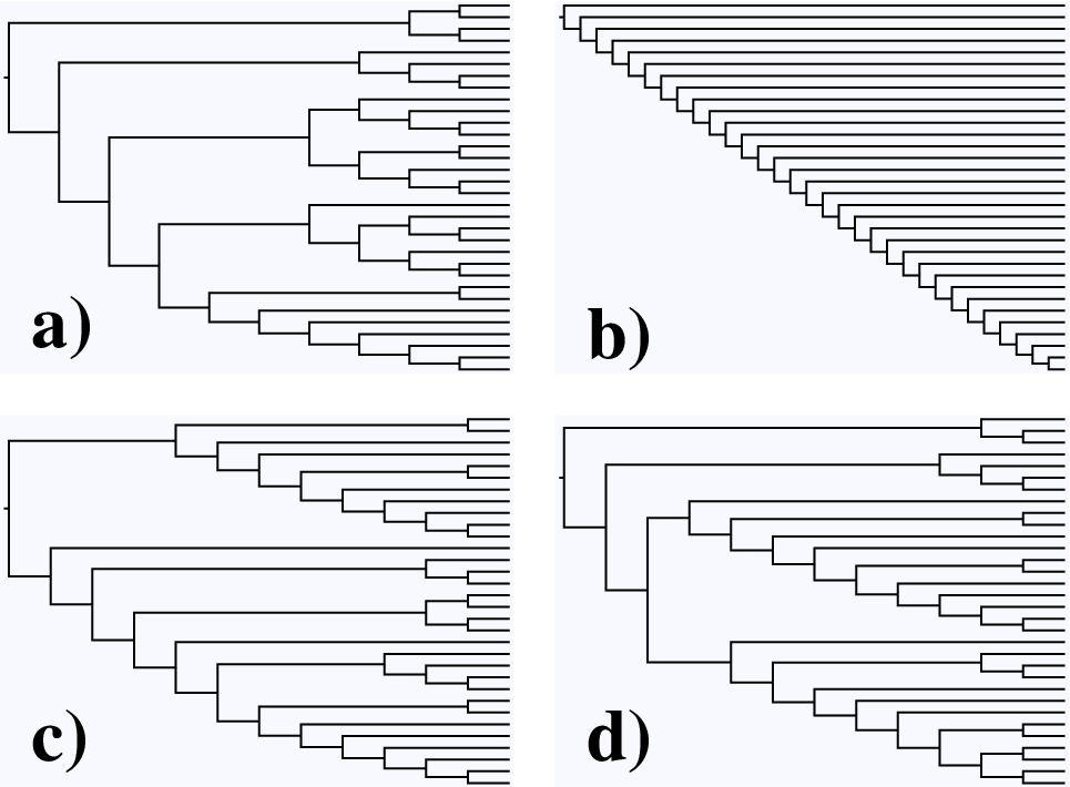
Ford [2006] introduced a model for recursive tree formation: At a given step in the process the tree is a set of leaves connected by terminal links to internal nodes, which are themselves connected by internal edges until reaching the root (the root itself is considered to have a single edge, which we count as internal, joining to the first bifurcating internal node; with this convention a tree of leaves has internal edges). Then, a probability of branching proportional to is assigned to each leaf, and proportional to to each internal edge. By normalization these probabilities are, respectively, , and . When a leaf is selected for branching, it gives birth to a couple of new ones, as in the ERM model. But when choosing an internal edge, a new leaf branches from it by the insertion in the edge of a new internal node. For we have the standard ERM model. For the completely unbalanced comb tree, in which all leaves branch successively from a main branch, is generated. Intermediate topologies are obtained for . Figure 2 shows examples of trees generated for different values of .
By considering the effect of the addition of new leaves on the distances between root and other nodes, Ford [2006] derived exact recurrence relationships which, when written in terms of the average depth, lead to:
| (2) |
is the mean depth of the leaves of a tree with leaves. By assuming a behavior at large , and expanding Eq. (2) in powers of , we get , so that
| (3) |
If the standard ERM behavior, Eq. (1), is recovered.
Figure 3 shows numerical results for the depth of trees generated with this model. Note that the predicted asymptotic behavior is attained but only at very large tree sizes, in general sizes much larger than the tree sizes of the examples shown in Fig. 2 and of the available empirical phylogenies. As analytically demonstrated [Ford, 2006] depth statistics of subtrees of given size extracted from a large tree behave as data from trees of that size directly generated by the alpha model algorithm.
While the Ford model gives a simple mechanism for scaling in trees with a tunable exponent, the dynamical rule of posterior insertion of inner nodes is hard to justify in the context of evolution (although one can think on the modelling of errors arising in phylogenetic reconstruction methods when incorrectly assigning a splitting to a non-existing ancestral species). This motivates the introduction of a new model described in the next section.
3 Activity model

In this section we show that tree shapes distinct from the ERM model may also result from a memory in terms of internal states of the nodes. The activity model proposed here is conceptually similar to the class of models suggested by Pinelis [2003]. However, the present model distinguishes only between active and inactive nodes and has a single parameter controlling the spread of activity.
Starting from a single node (the root), a binary tree is generated as follows. At each step, a leaf of the tree is chosen and branched into two new leaves. Each of the two new leaves, independently of the other, is set active with probability or inactive with probability . The branching leaf is chosen at random from the set of active leaves if this set is non-empty. Otherwise, is chosen at random from the set of all leaves. Figure 4 shows that for the model generates trees with mean depth growing as the square root of tree size (note the log-log scale). Figure 2 displays a small-size example of such trees. For values of below or above , seems to increase logarithmically with .
Here we give a simplified argument to understand the observed exponent of the distance scaling with system size in the case . At the time the growing tree has leaves in total, let be the expected sum of distances of active leaves from the root, and the analogous quantity for the inactive leaves. When a randomly chosen active leaf –at distance from root– branches, the expected increase of is
| (4) | |||||
Here the three terms of the second line are for the activation of two, one and zero of the new leaves, respectively. This expression is appropriate as far as the number of active nodes is not zero. Simultaneously, the expected change in during the same event is
| (5) | |||||
We now average over the different choices of the particular active leave that has been branched. This amounts to replacing in the above formulae by , the average depth of the active leaves in a tree of leaves. Writing , for , one would get a closed system for the quantities provided is expressed in terms of them. This can be done by writing , where is the expected number of active leaves in a tree of leaves. This expected value is used here as an approximation to the actual number of active leaves.
The recurrence equations for are specially simple in the most interesting case , since the dependence in disappears from one of the equations:
| (6) | |||||
| (7) |
The solution (with initial condition ) of Eq. (6) is simply:
| (8) |
Since the probabilities of an increment or decrement (by one unit) of the number of active leaves are the same and time-independent for , the number of active nodes performs a symmetric random walk with a reflecting boundary at 0 (this last condition arises from the prescription of setting active one node when the number of active nodes has reached zero in the previous step). For such random walk the expected value of active leaves increases as the square root of the number of steps. Since a new leaf is added at each time step, this leads to:
| (9) |
Combining (8) and (9) we obtain the average distance of active nodes from root at large tree sizes:
| (10) |
Now we can plug this result into Eq. (7), which can be solved recursively:
| (11) |
The totally averaged depth , which counts both the active and the inactive leaves, is
| (12) |
which explains the asymptotic behavior observed in Fig. 4 for .
We note that the growth dynamics presented here may be mapped to a branching process [Harris, 1963], with the difference that here the death (inactivation) of a node does not lead to its removal from the tree. The special case corresponds to a critical branching process.
4 Discussion
We have presented and studied two simple models which lead to non-logarithmic scaling of the tree depth. In contrast with many of the available models having this behavior [Banavar et al., 1999; Aldous, 2001; Blum & François, 2006; Ford, 2006] they are formulated as dynamical models involving growing trees, so that rules are given to obtain the tree at the next time step from the present state. Their study has been motivated by data from phylogenetic branching, and they are interesting additions to our present understanding of complex networks and trees.
A recent analysis of several evolutionary models including species competition [Stich & Manrubia, 2008] indicates that in these models correlations are finally destroyed by mutation processes and persist only for a finite correlation time. Thus sufficiently large trees would have a scaling behavior closer to the asymptotic ERM predictions. Since the largest phylogenies in databases such as TreeBASE have only some hundreds of leaves, it is possible that the observed imbalance and depth scaling is a finite-size regime. Nevertheless models going beyond the ERM scaling are needed at least to explain this finite-size regime, and also to elucidate the true asymptotic scaling behavior. Here, we have also observed large finite-size transients in the alpha model of Sect. 2.
The different types of scaling of depth with size can be interpreted as indicating different values of the (fractal) dimensionality of the trees. This is so because is a measure of the diameter of the tree, and because for a binary tree the total number of nodes is simply twice the number of leaves. Since the simplest definition of dimension of a network [Eguíluz et al., 2003] is given by the growth of the number of nodes as the diameter increases, , power law scaling of the type indicates that the tree can be thought as having a dimension . The logarithmic scaling in the ERM model is an example of the small-world behavior common to many network structures [Albert & Barabási, 2002], which is equivalent to having an effective infinite dimensionality, whereas the power law scaling reveals a finite dimension for the tree, which implies a more constrained mode of branching. The alpha model produces trees with tunable dimension from 1 to , and the critical activity model gives two-dimensional trees.
The final aim of the modelling of phylogenetic trees is to provide biological mechanisms explaining the branching topology of the Tree of Life. In this direction, the branching of internal edges in the Ford model has no obvious biological interpretation. The activity model puts the mechanisms of birth-death critical branching [Harris, 1963] within a framework of transitions between node internal states similar in spirit to the approach of Pinelis [2003]. The need to tune a parameter to attain the non-ERM critical behavior is however a limitation for its applicability. Much additional work is needed to identify the proper biological mechanisms behind evolutionary branching and adequate modelling of them.
Acknowledgments
We acknowledge financial support from the European Commission through the NEST-Complexity project EDEN (043251) and from MICINN (Spain) and FEDER through project FISICOS (FIS2007-60327).
References
- Albert & Barabási [2002] Albert, R. & Barabási, A.-L. [2002] “Statistical mechanics of complex networks.” Rev. Mod. Phys. 74, 47–97.
- Aldous [2001] Aldous, D. [2001] “Stochastic models and descriptive statistics for phylogenetic trees from Yule to today.” Stat. Sci. 16, 23–34.
- Banavar et al. [1999] Banavar, J. R., Maritan, A. & Rinaldo, A. [1999] “Size and form in efficient transportation networks.” Nature 399, 130–132.
- Blum & François [2006] Blum, M. G. B. & François, O. [2006] “Which random processes describe the Tree of Life? A large-scale study of phylogenetic tree imbalance.” Syst. Bot. 55, 685–691.
- Boccaletti et al. [2006] Boccaletti, S., Latora, V., Moreno, Y., Chavez, M. & Hwang, D.-U. [2006] “Complex networks: Structure and dynamics.” Phys. Rep. 424, 175–308.
- Burlando [1990] Burlando, B. [1990] “The fractal dimension of taxonomic systems.” J. Theor. Biol. 146, 99–114.
- Burlando [1993] Burlando, B. [1993] “The fractal geometry of evolution.” J. Theor. Biol. 163, 161–166.
- Caldarelli et al. [2004] Caldarelli, G., Caretta Cartozo, C., De Los Rios, P. & Servedio, V. D. P. [2004] “Widespread occurrence of the inverse square distribution in social sciences and taxonomy.” Phys. Rev. E 69, 035101.
- Capocci et al. [2008] Capocci, A., Rao, F. & Caldarelli, G. [2008] “Taxonomy and clustering in collaborative systems: The case of the on-line encyclopedia Wikipedia.” Europhys. Lett. 81, 28006.
- Cavalli-Sforza & Edwards [1967] Cavalli-Sforza, L. L. & Edwards, A. W. F. [1967] “Phylogenetic analysis: models and estimation procedures.” Evolution 21, 550–570.
- Cracraft & Donoghue [2004] Cracraft, J. & Donoghue, M. J. [2004] Assembling the Tree of Life (Oxford University Press).
- De Los Rios [2001] De Los Rios, P. [2001] “Power law size distribution of supercritical random trees.” Europhys. Lett. 56, 898–903.
- Eguíluz et al. [2003] Eguíluz, V. M., Hernández-García, E., Piro, O. & Klemm, K. [2003] “Effective dimensions and percolation in hierarchically structured scale-free networks.” Phys. Rev. E 68, 055102.
- Ford [2006] Ford, D. J. [2006] Probabilities on cladograms: introduction to the alpha model. Ph.D. thesis, Stanford University. Available from arXiv:math.PR/0511246.
- Garlaschelli et al. [2003] Garlaschelli, D., Caldarelli, G. & Pietronero, L. [2003] “Universal scaling relations in food webs.” Nature 423, 165–168.
- Guimerà et al. [2003] Guimerà, R., Danon, L., Díaz-Guilera, A., Giralt, F. & Arenas, A. [2003] “Self-similar community structure in a network of human interactions.” Phys. Rev. E 68, 065103.
- Harding [1971] Harding, E. F. [1971] “The probabilities of rooted tree-shapes generated by random bifurcation.” Adv. Appl. Prob. 3, 44–77.
- Harris [1963] Harris, T. E. [1963] The theory of branching processes (Springer-Verlag, Berlin, and Prentice-Hall, Inc., Englewood Cliffs, N.J.). Reprinted by Dover, NY, 1989 and 2002.
- Hernández-García et al. [2007] Hernández-García, E., Herrada, E. A., Rozenfeld, A. F., Tessone, C. J., Eguíluz, V. M., Duarte, C. M., Arnaud-Haond, S. & Serrao, E.A. [2007] “Evolutionary and ecological trees and networks.” In Nonequilibrium Statistical Mechanics and Nonlinear Physics: XV Conference on Nonequilibrium Statistical Mechanics and Nonlinear Physics, edited by Descalzi, O., Rosso, O. A. & Larrondo, H. A., volume 913 of AIP Conference Proceedings, pp. 78–83 (AIP).
- Herrada et al. [2008] Herrada, E. A., Tessone, C. J., Klemm, K., Eguíluz, V. M., Hernández-García, E. & Duarte, C. M. [2008] “Universal scaling in the branching of the tree of life.” PLoS ONE 3, e2757.
- Jain & Dubes [1988] Jain, A. & Dubes, R. [1988] Algorithms for Clustering Data (Prentice Hall, Englewood Cliffs, NJ).
- Klemm et al. [2005] Klemm, K., Eguíluz, V. M. & San Miguel, M. [2005] “Scaling in the structure of directory trees in a computer cluster.” Phys. Rev. Lett. 95, 128701.
- Klemm et al. [2006] Klemm, K., Eguíluz, V. M. & San Miguel, M. [2006] “Analysis of attachment model for directory and file trees.” Physica D 214, 149–155.
- Pinelis [2003] Pinelis, I. [2003] “Evolutionary models of phylogenetic trees.” Proc. R. Soc. Lond. B 270, 1425–1431.
- Rodriguez-Iturbe & Rinaldo [1997] Rodriguez-Iturbe, I. & Rinaldo, A. [1997] Fractal River Basins: Chance and Self-Organization (Cambridge University Press).
- Rozenfeld et al. [2008] Rozenfeld, A. F., Arnaud-Haond, S., Hernández-García, E., Eguíluz, V. M., Serrão, E. A. & Duarte, C. M. [2008] “Network analysis identifies weak and strong links in a metapopulation system.” Proc. Nat. Acad. Sci. 105, 18824–18829.
- Stevens [1974] Stevens, P. S. [1974] Patterns in Nature (Little Brown & Co, Boston).
- Stich & Manrubia [2008] Stich, M. & Manrubia, S. C. [2008] “Topological properties of phylogenetic trees in evolutionary models.” Preprint .
- West et al. [1997] West, G. B., Brown, J. H. & Enquist, B. J. [1997] “A general model for the origin of allometric scaling laws in biology.” Science 276, 122–126.
- Yule [1925] Yule, G. U. [1925] “A mathematical theory of evolution, based on the conclusions of Dr. J. C. Willis, F.R.S.” Phil. Trans. R. Soc. Lond. B 213, 21–87.