Bosonic Spectral Function in HTSC Cuprates:
Part I - Experimental Evidence for Strong Electron-Phonon Interaction
Abstract
In Part I we discuss accumulating experimental evidence related to the structure and origin of the bosonic spectral function in high-temperature superconducting (HTSC) cuprates near optimal doping. Some global properties of , such as number and positions of peaks, are extracted by combining optics, neutron scattering, ARPES and tunnelling measurements. These methods give convincing evidence for strong electron-phonon interaction (EPI) with in cuprates near optimal doping. Here we clarify how these results are in favor of the Eliashberg-like theory for HTSC cuprates near optimal doping.We argue that the neglect of EPI in some previous studies of HTSC was based on a number of deceptive prejudices related to the strength of EPI, on some physical misconceptions and misleading interpretation of experimental results.
In Part II we discuss some theoretical ingredients which are necessary to explain the experimental results related to pairing mechanism in optimally doped cuprates. These comprise the Migdal-Eliashberg theory for EPI in strongly correlated systems which give rise to the forward scattering peak. The latter is due to the combined effects of the weakly screened Madelung interaction in the ionic-metallic structure of layered cuprates and many body effects of strong correlations. While EPI is responsible for the strength of pairing the residual Coulomb interaction (by including spin fluctuations) triggers the d-wave pairing.
I Introduction
In spite of an unprecedentedly intensive experimental and theoretical study after the discovery of high-temperature superconductivity (HTSC) in cuprates there is, even twenty-two years after, no consensus on the pairing mechanism in these materials. At present there are two important experimental facts which are not under dispute: (1) the critical temperature in cuprates is high, with the maximum ; (2) the pairing in cuprates is d-wave like, i.e. with . On the contrary there is a dispute concerning the scattering mechanism which governs normal state properties and pairing in cuprates. To this end, we stress that in the HTSC cuprates, a number of properties can be satisfactorily explained by assuming that the quasi-particle dynamics is governed by some electron-boson scattering and in the superconducting state bosonic quasi-particles are gluing electrons in Cooper pairs. Which bosonic quasi-particles are dominating in the cuprates is the subject which will be discussed in this work. It is known that the electron-boson (phonon) scattering is well described by the Migdal-Eliashberg theory if the adiabatic parameter fulfills the condition , where is the electron-boson coupling constant, is the characteristic bosonic energy and is the electronic band width. The important characteristic of the electron-boson scattering is the Eliashberg spectral function (or its average ) which characterizes scattering of quasi-particle from to by exchanging bosonic energy . Therefore, in systems with electron-boson scattering the knowledge of this function is of crucial importance. There are at least two approaches differing in assumed gluing bosons. The first one is based on the electron-phonon interaction (EPI) [1], [2], [4], [5], [3] where mediating bosons are phonons and where the the average spectral function is similar to the phonon density of states . Note, is not the product of two functions although sometimes one defines the function which should approximate the energy dependence of the strength of the EPI coupling. There are numerous experimental evidence in cuprates which support the dominance of the EPI scattering mechanism with a rather large coupling constant and which will be discussed in detail below. In the EPI approach is extracted from tunnelling measurements in conjunction with IR optical measurements. We stress again that the Migdal-Eliashberg theory is well justified framework for EPI since in most superconductors the condition is fulfilled. The HTSC are on the borderline and it is a natural question - under which condition can high Tc be realized in the non-adiabatic limit ? The second approach [6] assumes that EPI is too weak to be responsible for high in cuprates and it is based on a phenomenological model for spin-fluctuation interaction () as the dominating scattering mechanism, i.e. it is a non-phononic mechanism. In this approach the spectral function is proportional to the imaginary part of the spin susceptibility , i.e. . NMR spectroscopy and magnetic neutron scattering give that in HTSC cuprates is peaked at the antiferromagnetic wave vector and this property is favorable for d-wave pairing. The theory roots basically on the strong electronic repulsion on Cu atoms, which is usually studied by the Hubbard model or its (more popular) derivative the t-J model. Regarding the possibility to explain high Tc solely by strong correlations, as it is reviewed in [7], we stress two facts. First, at present there is no viable theory which can justify these (non-phononic) mechanisms of pairing. Second, the central question in this approach is - do models based on the Hubbard Hamiltonian show up superconductivity at sufficiently high critical temperatures ( ) ? A number of numerical studies of these models offer a negative answer. For instance, the sign-free variational Monte Carlo algorithm in the 2D repulsive () Hubbard model gives no evidence for HTSC, neither the BCS- nor Berezinskii-Kosterlitz-Thouless (BKT)-like [8]. At the same time, similar calculations show that there is a strong tendency to superconductivity in the attractive () Hubbard model for the same strength of , i.e. at finite temperature in the 2D model with the BKT superconducting transition is favored. Concerning HTSC in the model, various numerical calculations such as Monte Carlo calculations of the Drude spectral weight [9] and high temperature expansion [10] have shown that there is no superconductivity at temperatures characteristic for cuprates and if it exists must be rather low - few Kelvins. These numerical results tell us that the lack of high (even in BKT phase) in the repulsive () single-band Hubbard model and in the model is not only due to thermodynamical -fluctuations (which at finite T suppress and destroy superconducting phase coherence in large systems) but it is mostly due to an inherent ineffectiveness of strong correlations to produce solely high in cuprates. These numerical results certainly mean that the simple single-band Hubbard, as well as its derivative the t-J model, are insufficient to explain the pairing mechanism in cuprates and some other ingredients must be included. Having in mind these facts there is no room at present for any kind of celebration of the victory of non-phononic mechanisms of pairing as some prefer to do.
Since is as a rule strong in oxides, then it is plausible that it should be accounted for in cuprates at least in the normal metallic state. As it will be argued later on, the experimental support for the importance of EPI comes from optics, tunnelling, and recent ARPES measurements [11]. It is worth mentioning that recent ARPES activity was a strong impetus for renewed experimental and theoretical studies of EPI in cuprates. However, in spite of accumulating experimental evidence for importance of EPI with , there are occasionally reports which doubt its importance in cuprates. This is the case with recent interpretation of some optical measurements in terms of SFI only [12] and with LDA band structure calculations [13], [14], where both claim that EPI is negligibly small, i.e. .
The paper is organized as follows. There are two parts - in Part I we will mainly discuss experimental results in cuprates near optimal doping and minimal theoretical explanations which are related to the spectral function as well to the transport spectral function and how these are related to EPI in cuprates. In this work we consider mainly those direct one-particle and two-particles probes of low energy quasi-particle excitations (by including gap and pseudogap) and scattering rates which give informations on the structure of the spectral functions and in systems near optimal doping. These are angle-resolved photoemission (), various arts of tunnelling spectroscopies such as superconductor/insulator/ normal metal () junctions and break junctions, scanning-tunnelling microscope spectroscopy (), infrared () and Raman optics, inelastic neutron scattering () etc. We shall argue that these direct probes give evidence for a rather strong EPI in cuprates as dominating scattering mechanism of quasi-particles. Some other experiments on EPI are also discussed in order to complete the arguments for the importance of EPI in cuprates. The detailed contents of Part I is the following. In Section II we discuss some prejudices related to and the Fermi-liquid behavior of HTSC cuprates. We argue that any non-phononic mechanism of pairing should have very large bare critical temperature in the presence of the large EPI coupling constant, , if its spectral function is weakly momentum dependent, i.e. if . The fact that EPI is large in the normal state of cuprates and the condition that it must conform with d-wave pairing implies inevitably that EPI in cuprates must be strongly momentum dependent. In Section III we discuss direct and indirect experimental evidence for the importance of EPI and for the weakness of SFI in cuprates. These are:
(A) Magnetic neutron scattering measurements - These measurements provide dynamic spin susceptibility which is in the phenomenological approach [6] related to the Eliashberg spectral function, i.e. . We stress that such an approach can be qualitatively justified only in the weak coupling limit, , where is the band width. Here we discuss experimental results which give evidence for strong rearrangement (with respect to ) of by doping toward the optimal doped HTSC [16]. It turns out that in the optimally doped cuprates with is drastically suppressed compared to that in slightly underdoped ones with , and this is strong evidence for the smallness of the SFI coupling constant.
(B) Optical conductivity measurements - From these measurements one can extract the transport relaxation rate and indirectly an approximative shape of the transport spectral function . In that respect we discuss: (i) the misleading concept concerning the relation between the optical relaxation rate and the quasi-particle relaxation rate . This (misleading) concept has been appearing repeatedly in the last twenty years despite the fact that this controversy is resolved many years ago [17], [18], [19], [1], [2], [44]; (ii) some methods of extraction of the optical spectral function from optical reflectivity measurements. It turns out that the width and the shape of the extracted favor EPI; (iii) the restricted sum-rule for the optical weight as a function of temperature which can also be explained by strong [20], [21]; (iv) good agreement with experiments of the temperature dependence of the resistivity calculated with the extracted . Recent femtosecond time-resolved optical spectroscopy in gives additional evidence for importance of EPI and ineffectiveness of SFI [22].
(C) ARPES measurements and EPI - From these measurements one can extract the self-energy from which one can extract some properties of . Here we discuss the following items: (i) appearance of the nodal and anti-nodal kinks in optimally and slightly underdoped cuprates, as well as the structure of the ARPES self-energy () and its isotope dependence, which are all due to EPI; (ii) appearance of different slopes of at low () and high energies () which can be explained with strong EPI; (iii) formation of small polarons in the undoped HTSC which is due to strong EPI - this gives rise to phonon side bands which are clearly seen in ARPES of undoped HTSC.
(D) Tunnelling spectroscopy - It is well known that this method is of an immense importance in obtaining the spectral function from tunnelling conductance. In this part we discuss the following items: (i) extraction of the Eliashberg spectral function with from the tunnelling conductance of break-junctions [23]-[29] which gives that the maxima of coincide with the maxima in the phonon density of states; (ii) the presence of the dip in dI/dV in STM which shows the pronounced oxygen isotope effect and important role of these phonons: (iii) the presence of fine and doping independent structure in I(V) characteristics due to phonon emission by the Josephson current in layered HTSC cuprates with intrinsic Josephson junctions.
(E) Phonon neutron scattering measurements - From these experiments one can extract the phonon density of state and strengths of the quasi-particle coupling with various phonon modes. Here we argue, that the large softening and broadening of the half-breathing Cu-O bond-stretching phonon, of apical oxygen phonons and of oxygen buckling phonons (in LSCO, BISCO,YBCO) cannot be explained by LDA. It is curious that the magnitude of softening can be partially obtained by LDA but the calculated widths of some important modes are an order of magnitude smaller than the neutron scattering data show. This remarkable fact implies the inadequacy of LDA in strongly correlated systems and a more sophisticated many body theory for EPI is needed. This problem will be discussed in more details in Part II [15]. In Section IV brief summary of the Part I is given. Since we are dealing with electron-boson scattering in cuprate near optimal doping, then in Section V - Appendix we introduce the reader briefly into the Migdal-Eliashberg theory for superconductors (and normal metals) where the quasi-particle spectral function and the transport spectral function are defined.
Finally, at the end of the day one poses a question - do the experimental results of the above enumerated spectroscopic methods allow a building of a satisfactory and physically reasonable microscopic theory for basic scattering and pairing mechanism in cuprates? The posed question is very modest compared with a much stringent request for the theory of everything - which would be able to explain all properties of HTSC materials. Such an ambitious project is not realized even in those low-temperature conventional superconductors where it is definitely proved that the pairing is due to EPI and many properties are well accounted for by the Migdal-Eliashberg theory. Let us mention only two examples. First, the experimental value for the coherence peak in the microwave response at in is much higher than the theoretical value obtained by the Migdal-Eliashberg theory [31]. So to say, the theory explains the coherence peak at in qualitatively but not quantitatively. However, the measurements at higher frequency are in agreement with the Migdal-Eliashberg theory [32]. Second, the experimental boron (B) isotope effect in (with ) is much smaller than the theoretical value, i.e. , although the pairing is due solely by EPI for boron vibrations [33]. Since the theory of everything is impossible in the complex materials such as HTSC cuprates in Part I and II we shall not discuss those phenomena which need much more microscopic details and/or more sophisticated many-body theory. These are selected by chance: (i) peculiarities of the coherence peak in the microwave response in HTSC cuprates, which is peaked at much smaller than , contrary to the case of LTSC where it occurs near ; (ii) dependence on the number of in the unit cell; (iii) temperature dependence of the Hall coefficient; (iv) distribution of states in the vortex core, etc. However, in a separate paper - Part II [15] we shall discuss some minimal theoretical concepts which can explain at least qualitatively and semi-quantitatively results related to the above enumerated spectroscopic methods. Due to the presence of strong correlations and quasi-2D electronic structure some of these concepts go beyond the LDA approach. In our opinion at this stage of the HTSC physics some important ingredients of the future theory are already recognized. These are: (1) very peculiar quasi-2D ionic-metallic structure with a rather weak screening along the c-axis, which is a prerequisite for strong EPI; (2) strong Coulomb interaction and correlations which are responsible for strong magnetism in undoped cuprates and for important renormalizations of EPI. Since both ingredients belong to the class of strong coupling problems, at present there is no quantitative theory and therefore we must rely on approximative and model theories. Even these approaches allow us qualitative (and semi-quantitative) explanations of some important properties which are due to the interplay of EPI and strong correlations. The latter two cause the appearance of momentum dependent EPI - peaked at small transfer momenta [2]. Based on such an approach we are able to explain (understand) at least qualitatively some very puzzling experimental results, for instance: (a) why is d-wave pairing realized in the presence of strong EPI? (b) why is the transport coupling constant () smaller than the pairing one , i.e. ? (c) Why is the mean-field (one-body) LDA approach unable to give reliable values for the EPI coupling constant in cuprates and how many-body effects help; (d) why is d-wave pairing robust in presence of non-magnetic impurities and defects? (e) why the ARPES nodal and antinodal kinks are differently renormalized in the superconducting states?
In real materials there are numerous experimental evidence for nanoscale inhomogeneities in HTSC oxides . For instance recent STM experiments show rather large gap dispersion at least on the surface of BISCO crystals [30] giving rise for a pronounced inhomogeneity of the superconducting order parameter, i.e. where is the relative momentum of the Cooper pair and is the center of mass of Cooper pairs. One possible reason for the inhomogeneity of and disorder on the atomic scale can be due to extremely high doping level of in HTSC cuprates which is many orders of magnitude larger than in standard semiconductors ( vs carrier concentration). There are some claims that high is exclusively due to these inhomogeneities (of an extrinsic or intrinsic origin) which may increase EPI [34], while other try to explain high within the inhomogeneous Hubbard or t-J model. In Part II [15] we argue that the concept of an increase of Tc by inhomogeneity is ill-defined, since the increase of is defined with respect to the average value . However, the latter quantity is experimentally not well defined and an alleged increase of by the material inhomogeneity cannot be tested at all.
II EPI vs non-phononic mechanisms - facts vs prejudices
Concerning the high in cuprates, one of the central questions is - which interaction(s) is(are) responsible for strong quasi-particle scattering in the normal state and for the superconducting pairing? In the last twenty-two years, the scientific community was overwhelmed by all kinds of (im)possible proposed pairing mechanisms, most of which are hardly verifiable in any material, if at all. This trend is still continuing nowadays (although with smaller slope), in spite of the fact that the accumulated experimental results eliminate all but few.
A. Fermi vs non-Fermi liquid in cuprates
After discovery of HTSC in cuprates there was a large amount of evidence on strong scattering of quasi-particles which contradicts the canonical (popular but narrow) definition of the Fermi liquid, thus giving rise to numerous proposals of the so called non-Fermi liquids, such as Luttinger liquid, RVB theory, marginal Fermi liquid, etc. In our opinion there is no need for these radical approaches in explaining basic physics in cuprates at least in optimally, slightly underdoped and overdoped metallic and superconducting HTSC cuprates. This subject will be discussed more in Part II and here we give some clarifications related to the dilemma of Fermi vs non-Fermi liquid. The definition of the canonical Fermi liquid (based on the Landau work) in interacting Fermi systems comprises the following properties: (1) there are quasi-particles with charge , spin and low-laying energy excitations which are much larger than their inverse life-times, i.e. . Since the level width of the quasi-particle is negligibly small, this means that the excited states of the Fermi liquid are placed in one-to-one correspondence with the excited states of the free Fermi gas; (2) at there is an energy level with the Fermi surface at which and the Fermi quasi-particle distribution function has finite jump; (3) the number of quasi-particles under the Fermi surface is equal to the total number of conduction particles (we omit here other valence and core electrons) - the Luttinger theorem; (4) the interaction between quasi-particles are characterized with a few (Landau) parameters which describe low-temperature thermodynamics and transport properties. Having this definition in mind one can say that if fermionic quasi-particles interact with some bosonic excitation (for instance with phonons) and if the coupling is sufficiently strong, then the former are not described by the canonical Fermi liquid since at energies and temperatures of the order of the Debay temperature (more precisely ), i.e. for one has and the quasi-particle picture (in the sense of the Landau definition) is broken down. In that respect an electron-boson system can be classified as a non-canonical Fermi liquid for sufficiently strong electron-boson coupling. It is nowadays well known that for instance Al, Zn are weak coupling systems since for one has and they are well described by the Landau theory. However, the electron-phonon system is satisfactory described by the Migdal-Eliashberg theory and the Boltzmann theory, where thermodynamic and transport properties depend on the spectral function and its higher momenta. Since in HTSC cuprates the electron-boson (phonon) coupling is rather strong and is large, i.e. of the order of characteristic boson energies (), , then it is natural that in the normal state (at ) we deal inevitably with a strong interacting non-canonical Fermi liquid which is at least qualitatively and semi-quantitatively described by the Migdal-Eliashberg theory. In order to justify this statement we shall in the following elucidate some properties in more details by studying optical, ARPES, tunnelling and other experiments.
B. Prejudice on the limitation of the strength of EPI
In spite of reach experimental evidence in favor of strong EPI in HTSC oxides there was a disproportion in the research activity (especially theoretical) in the past, since the investigation of the SFI mechanism of pairing prevailed in the literature. This retrograde trend was partly due to an incorrect statement in [35] on the possible upper limit of Tc in the phonon mechanism of pairing. Since in the past we have discussed this problem thoroughly in numerous papers - for the recent one see [36], we shall outline here the main issue and results only.
It is well known that in an electron-ion crystal, besides the attractive EPI, there is also repulsive Coulomb interaction. In case of an isotropic and homogeneous system with weak quasi-particle interaction, the effective potential in the leading approximation looks like as for two external charges () embedded in the medium with the total longitudinal dielectric function ( is the momentum and is the frequency) [37], i.e.
| (1) |
In case of strong interaction between quasi-particles, the state of embedded quasi-particles changes significantly due to interaction with other quasi-particles, giving rise to . In that case depends on other (than ) response functions. However, in the case when Eq.(1) holds, i. e. when the weak-coupling limit is realized, is given by [118], [37]. Here, is the EPI coupling constant, is an average phonon frequency and is the Coulomb pseudo-potential, ( is the Fermi energy). The couplings and are expressed by
| (2) |
where is the density of states at the Fermi surface and is the Fermi momentum - see more in [1]. In [35] it was claimed that lattice stability of the system with respect to the charge density wave formation implies the condition for all . If this was correct then from Eq.(2) it follows that , which limits the maximal value of Tc to the value . In typical metals and if one accepts the statement in [35], i.e. that , one obtains . The latter result, if it would be true, means that EPI is ineffective in producing not only high-Tc superconductivity but also low-temperature superconductivity (LTS). However, this result is apparently in conflict first of all with experimental results in LTSC, where in numerous systems and . For instance, is realized in alloy which is definitely much higher than .
Moreover, the basic theory tells us that is not the response function [37]. Namely, if a small external potential is applied to the system it induces screening by charges of the medium and the total potential is given by which means that is the response function. The latter obeys the Kramers-Kronig dispersion relation which implies the following stability condition: for , i.e. either or . This important theorem invalidates the above restriction on the maximal value of Tc in the EPI mechanism. We stress that the condition is not in conflict with the lattice instability. For instance, in inhomogeneous systems such as crystal, the total longitudinal dielectric function is matrix in the space of reciprocal lattice vectors (), i.e. , and is defined by . It is well known that in dense metallic systems with one ion per cell (such as metallic hydrogen ) and with the electronic dielectric function , one has [38]
| (3) |
At the same time the frequency of the longitudinal phonon is given by
| (4) |
where is the ionic plasma frequency, is the local (electric) field correction - see Ref. [38]. The real condition for lattice stability requires that , which implies that for one has . The latter condition gives automatically . Furthermore, the calculations [38] show that in the metallic hydrogen crystal, for all . Moreover, the analyzes of crystals with more ions per unit cell [38] gives that is more a rule than an exception - see Fig. 1. The physical reason for are local field effects described above by . Whenever the local electric field acting on electrons (and ions) is different from the average electric field , i.e. , there are corrections to (and to ) which may lead to .

The above analysis tells us that in real crystals can be negative in the large portion of the Brillouin zone giving rise to in Eq.(2). This means that the dielectric function does not limit in the phonon mechanism of pairing. This result does not mean that there is no limit on Tc at all - see more in [36] and references therein. We mention in advance that the local field effects play important role in HTSC oxides, due to their layered structure with very unusual ionic-metallic binding, thus giving rise to large - see more in the subsequent sections. It is pertinent to note that one of the author of [35] recognizes the possibility and in [39] even makes interesting proposals for compounds with large EPI and , while the other author [40] still ignores rigors of scientific arguments and negates importance of EPI in HTSC cuprates.
In conclusion we point out that there are no theoretical and experimental arguments for ignoring EPI in HTSC cuprates. To this end it is necessary to answer several important questions which are related to experimental findings in HTSC cuprates (oxides): (1) if EPI is responsible for pairing in HTSC cuprates and if superconductivity is of type, how are these two facts compatible? (2) why is the transport EPI coupling constant (entering resistivity) much smaller than the pairing EPI coupling constant (entering Tc), i.e. why one has ? (3) is high Tc possible for a moderate EPI coupling constant, let say for , and under which conditions? (4) if EPI is ineffective for pairing in HTSC oxides, inspite of , why it is so?
C. Is a non-phononic pairing realized in HTSC?
Regarding EPI one can pose a question - whether it contributes significantly to d-wave pairing in cuprates? Surprisingly, despite numerous experiments in favor of EPI, a number of researchers still believe that EPI is irrelevant for pairing [6]. This belief is mainly based: (i) on the, previously discussed, incorrect lattice stability criterion, which implies small EPI; (ii) on the well established experimental fact that d-wave pairing is realized in cuprates [41], which is believed to be incompatible with EPI. Having in mind that EPI in HTSC is strong with (see below), we assume for the moment that the leading pairing mechanism in cuprates, which gives d-wave pairing, is due to some non-phononic mechanism, like the exitonic one, with the high energy gluing boson () and with the bare critical temperature and look for the effect of EPI. If EPI is isotropic, like in most LTSC materials, then it would be very detrimental for d-wave pairing - the pair breaking effect. In the case of dominating isotropic EPI in the normal state and the exitonic-like pairing, then near the linearized Eliashberg equations have an approximative form for weak non–phonon interaction (with the characteristic frequency )
| (5) |
For pure d-wave pairing one has and which gives the equation for Tc - see [1]
| (6) |
Here is the di-gamma function. At temperatures near one has and the solution of Eq. (6) is approximately , which means that for and the bare due to the non-phononic interaction must be very large, i.e. .
Concerning other non-phononic mechanisms, such as the SFI one, the effect of the isotropic EPI in the framework of Eliashberg equations was studied numerically in [42]. The latter is based on Eqs.(42-44) in Appendix A. with kernels
| (7) |
| (8) |
where is taken in the FLEX approximation [43]. The calculations [42] confirm the very detrimental effect of the isotropic EPI on the d-wave pairing due to SFI. For the bare SFI and the calculations give very small . These results tell us that a more realistic pairing interaction must be operative in cuprates and that EPI is strongly momentum dependent [45]. Only in that case is strong EPI conform with d-wave pairing, either as its main cause or as a supporter of a non-phononic mechanism. In Part II we shall argue that the strongly momentum dependent EPI is the main player in cuprates providing the strength of the pairing mechanism, while the residual Coulomb interaction and SF, although weaker, trigger it to d-wave pairing.
III Experimental evidence for strong EPI and weak SFI
In the following we discuss some important experiments which give evidence for strong EPI in cuprates. Before doing it; we shall discuss some magnetic neutron scattering measurements in cuprates whose results are against the SFI mechanism of pairing. The experimental results related to the pronounced imaginary part of the susceptibility at the AF wave vector were interpreted in a number of papers as a support for the SFI mechanism for pairing [6]. We briefly explain inadequacy of such an interpretation.
III.1 Magnetic neutron scattering and the spin fluctuation spectral function
A. SFI affects very little
Before discussing experimental results in cuprates on the imaginary part of the spin susceptibility we point out that in theories based on spin fluctuations the effective pairing potential , which is repulsive, is assumed in the form [6]
| (9) |
This form of can be theoretically justified in the weak coupling limit () only. This mechanism of pairing could be effective in cuprates only if the spin susceptibility (spectral function) Im is strongly peaked at the AF wave vector . What is the experimental situation? The breakthrough came from magnetic neutron scattering experiments on by Bourges group [16]. They showed that (the odd part of the spin susceptibility in the bilayer system) at is strongly dependent on the hole doping as it is shown in Fig. 2.


By varying doping there is a huge rearrangement of in the frequency interval which is important for superconducting pairing, let say as it is seen in the last two curve in Fig. 2(top). At the same time there is only a small variation of the corresponding critical temperature ! For instance, in the underdoped crystal Im, and , is much larger than that in the near optimally doped , i.e. , although the difference in the corresponding critical temperatures is very small, i.e. (in ) and (in ). This pronounced rearrangement and decrease of Im by doping, but a negligible change in in YBCO is clearly seen in Fig. 2(top), which is strong evidence against the mechanism of pairing. These results in fact mean that the coupling constant is small, i.e. , and the pairing mechanism is ineffective in cuprates. We stress that in the phenomenological theory of the SFI pairing [6], an unrealistically large coupling was assumed which gives . The latter value cannot be justified neither experimentally nor theoretically. Let us add that the anti-correlation between the decrease of and increase of by increasing doping toward the optimal value is also present in the NMR spectral function which determines the longitudinal relaxation rate - see [2]. This result additionally disfavors the SFI model of pairing [6], i.e. the strength of pairing interaction is little affected by SFI. As we shall discuss below the role of SFI together with the stronger direct Coulomb interaction is to trigger d-wave pairing.
A less direct argument for smallness of the SFI coupling constant, i.e. and comes from other experiments related to the magnetic resonance peak in the superconducting state, and this will be discussed next.
B. Ineffectiveness of the magnetic resonance peak
In the superconducting state of optimally doped YBCO and BISCO, is significantly suppressed at low frequencies except near the resonance energy where a pronounced narrow peak appears - the magnetic resonance peak. We stress that there is no magnetic resonance peak in LSCO sand consequently one can question the importance of the resonance peak in the scattering processes. The relative intensity of this peak (compared to the total one) is small, i.e. - see Fig 2 (bottom). In underdoped cuprates this peak is present also in the normal state as it is seen in Fig 2 (top). After the discovery of the resonance peak there were attempts to relate it: (i) to the origin of the superconducting condensation energy and (ii) to the kink in the energy dispersion or the peak-dimp structure in the ARPES spectral function. In order that the property (i) holds it is necessary that the peak intensity is small [46]. is obtained by equating the condensation energy with the change of the magnetic energy in the superconducting state, i.e. , where
| (10) |
By taking and the realistic value , one obtains . However, such a small intensity cannot be responsible for the anomalies in ARPES and optical spectra since it gives rise to small coupling constant for the interaction of holes with the resonance peak, i.e. . Such a small coupling does not affect superconductivity. Moreover, by studying the width of the resonance peak one can extract the SFI coupling constant . Thus, the magnetic resonance disappears in the normal state of the optimally doped YBCO, which can be qualitatively understood by assuming that its broadening scales with the resonance energy , i.e. , where the line-width is given by [46]. This limits to . We stress that the obtained is much smaller than the one assumed in the phenomenological spin-fluctuation theory [6] where , but much larger than in [46] (where ). The smallness of comes out also from the analysis of the antiferromagnetic state in underdoped metals of LSCO and YBCO [47], where the small magnetic moment points to an itinerant antiferromagnetism with small coupling constant . The conclusion is that the magnetic resonance in the optimally doped YBCO is a consequence of the onset of superconductivity and not its cause.
There is also a principal reason against the pairing due to the resonance peak at least in optimally doped cuprates. Since its intensity near is vanishingly small, though not affecting pairing at the second order phase transition at , then if it would be the origin for superconductivity the phase transition at Tc would be first order, contrary to experiments. Recent ARPES experiments give evidence that the magnetic resonance cannot be related to the kinks in ARPES spectra [48], [49] - see the discussion below.
III.2 Optical conductivity and EPI
Optical spectroscopy gives information on optical conductivity and on two-particle excitations, from which one can indirectly extract the transport spectral function . Since this method probes bulk sample (on the skin depth), contrary to ARPES and tunnelling methods which probe tiny regions ( Å) near the sample surface, this method is very indispensable. However, is not a directly measured quantity but it is derived from the reflectivity with the transversal dielectric tensor . Here, is the high frequency dielectric function, describes the contribution of the lattice vibrations and describes the optical (dynamical) conductivity of conduction carriers. was usually measured in the limited frequency interval . Therefore, some physical modelling for is needed in order to guess it outside this range - see more in reviews [1], [2]. This was the reason for numerous inadequate interpretations of optic measurements in cuprates, as well as the misconceptions and misinterpretations that will be uncover below. An illustrative example for this claim is large dispersion in the reported value of - from to , i.e. almost three orders of magnitude - see discussion in [50]. This tells us also that in some periods science suffers from a lack of rigorousness and objectiveness. However, it turns out that measurements of in conjunction with elipsometric measurements of at high frequencies allows reliable determination of .
1. Transport and quasiparticle relaxation rates
The widespread misconception in studying the quasi-particle scattering in cuprates was an ad hoc assumption that the transport relaxation rate is equal to the quasi-particle relaxation rate , in spite of the well known fact that [17]. This incorrect assumption led to the abandoning of EPI as relevant scattering mechanism in cuprates. Although we have discussed this problem several times before, we want to do it again, since the correct understanding of the scattering mechanism in cuprates will take us forward in understanding of the pairing mechanism.
The dynamical conductivity consists of two parts, i.e. where describes interband transitions which contribute at higher frequencies, while is due to intraband transitions which are relevant at low frequencies . (In measurements the frequency is usually given in , where the following conversion holds: .) The experimental data for in cuprates are usually processed by the generalized (extended) Drude formula [17], [51], [18], [19]
| (11) |
which is a useful representation for systems with single band electron-boson scattering which is justified in HTSC cuprates - see the discussion below. (The usefulness of introducing the optic relaxation will be discussed in Appendix B.) Here, enumerates the plane axis, , and are the electronic plasma frequency, the transport (optical) scattering rate and the optical mass, respectively. Very frequently, the quantity [51], which is determined from the half-width of the Drude-like expression for , was analyzed since it is independent of . In the weak coupling limit , the formula for conductivity given in Eqs. (64-67) can be written in the form of Eq.(11) where reads [18]-[19]
| (12) |
Here is the Bose distribution function. (For the explicit form of the transport mass see [17], [18], [19], [1], [2].) In the presence of impurity scattering one should add to . It turns out that Eq.(12) holds within a few percents also for large . Note, that and the index enumerates all scattering bosons - phonons, spin fluctuations, etc. For comparison, we give the quasi-particle scattering rate
| (13) |
where is the Fermi distribution function. By comparing Eq.(13) and Eq.(12), it is seen that and are different quantities, , i.e. the former describes the relaxation of Bose particles (electron-hole pairs) while the latter one the relaxation of Fermi particles. This difference persists also at where one has (due to simplicity we omit in the following summation over ) [17]
| (14) |
and
| (15) |
In the case of EPI, the above equations give that for while (as well as ) is monotonic growing for , where is the maximal phonon frequency. This is clearly seen by comparing , and which are calculated for the EPI spectral function extracted from tunnelling experiments in YBCO (with ) [23] - see Fig. 3.


The results shown in Fig. 3 clearly demonstrate the physical difference between two scattering rates and . It is also seen that is more a linear function of than . From these calculations one concludes that the quasi-linearity of (and ) is not in contradiction with the EPI scattering mechanism but it is in fact a natural consequence of EPI. We stress that such behavior of and , shown in Fig. 3, is in fact not exceptional for HTSC cuprates but it is generic for many metallic systems, for instance 3D metallic oxides, low temperature superconductors such as , , etc. - see more in [1], [2].
Let us discuss briefly the experimental results for and and compare these with theoretical predictions obtained by using a single band model and from tunnelling data with the EPI coupling [23]. In the case of YBCO the agreement between measured and calculated is very good up to frequencies which confirms the importance of EPI in scattering processes. For higher frequencies, where a mead infrared peak appears, it is necessary to account for interband transitions [1]. In optimally doped [52] the experimental results for are explained theoretically by assuming that the EPI spectral function , where is the phononic DOS in BISCO while , and - see Fig. 4(a). The agreement is rather good. At the same time the fit of by the marginal Fermi liquid fails as it is evident in Fig. 4(b).


Now we will comment on the so called pronounced linear behavior of (and ) which served in the past for numerous inadequate conclusions. We stress that the measured quantity is reflectivity and derived ones are , and , which are very sensitive to the value of the dielectric constant . This is clearly demonstrated in Fig. 5 for Bi2212 where it is seen that (and ) for is linear up to much higher than in the case .

In some experiments [53], [54] (and ) is linear up to very high which means that the ion background and interband transitions (contained in ) are not properly taken into account since it is assumed too small . The recent elipsometric measurements on YBCO [55] give the reliable value for . The latter gives rise to a much less spectacular linearity in the relaxation rates than it was the case immediately after the discovery of HTSC cuprates.
Furthermore, we would like to comment on two points concerning , , and their interrelations. First, the parametrization of with the generalized Drude formula in Eq.(11) and its relation to the transport scattering rate and the transport mass is useful if we deal with electron-boson scattering in a single band problem. In [19] it is shown that of a two-band model with only elastic impurity scattering can be represented by the generalized (extended) Drude formula with and dependence of effective parameters , despite the fact that the inelastic electron-boson scattering is absent. To this end we stress that the single-band approach is fully justified for a number of HTSC cuprates such as LSCO, BISCO etc. Second, at the beginning we said that and are physically different quantities and it holds . In order to give the physical picture and qualitative explanation we assume that . In that case the renormalized frequencies, the quasi-particle one (for the definition of see Appendix A.) and the transport one - defined above, are related and at , they are given by [17], [19]
| (16) |
It gives the relation between and , and respectively
| (17) |
| (18) |
The physical meaning of Eq.(16) is the following: in optical measurements one photon with the energy is absorbed and two excited particles (electron and hole) are created above and below the Fermi surface. If the electron has energy and the hole , then they relax as quasi-particles with the renormalized . Since takes values then the optical relaxation is the energy-averaged according to Eq.(16). The factor 2 is due to the two quasi-particles, electron+hole. At finite , the generalization reads [17], [19]
| (19) |
2. Inversion of the optical data and
In principle, the transport spectral function can be precisely extracted from , i.e. , only at , which follows from Eq.( 14)
| (20) |
However, real measurements are performed at finite (and also at ) and the inversion procedure is in principle an ill-posed problem since is the deconvolution of the inhomogeneous Fredholm integral equation of the first kind with the temperature dependent Kernel in Eq.(12). An ill-posed mathematical problem, like this one, is very sensitive to input since experimental data contain less information than one needs. This can cause the fine structure of gets blurred in the extraction procedures and it can be temperature dependent even when the true is independent. In the context of HTSC cuprates, this problem was first studied in [18], [19] with the following results: (1) the extracted shape of in is not unique and it is temperature dependent, i.e. at higher the peak structure is smeared and only a single peak (slightly shifted to higher ) is present. For instance, the experimental data of in YBCO were reproduced by two different spectral functions , one with single peak and the other with three peaks structure as it is shown in Fig. 6 The similar situation is realized in optimally doped BISCO as it is seen in Fig. 7. It is important to stress that the width of the extracted in both compounds coincide with the width of the phonon density of states [18], [19], [56]; (2) the upper energy bound for can be extracted with certainty and it coincides approximately with the maximal phonon frequency in cuprates as it is seen in Figs. 6-7.


These results undoubtedly demonstrate the importance of EPI in cuprates [18], [19], [1]. We point out that the width of which is extracted from the optical measurements [18], [19], [1] coincides with the width of the quasi-particle spectral function obtained in tunneling and ARPES spectra (which we shall discuss below), i.e. both functions are spread over the energy interval . Since in cuprates this interval coincides with the width in the phononic density of states and since the maxima of and almost coincide, this is further strong evidence for the dominance of EPI.
To this end, we would like to comment on two important points. First, in some reports [59],[12], [60] it was assumed that of cuprates can be extracted also in the superconducting state by using Eq. (20). However, Eq. (20) holds exclusively in the normal state (at T=0) since can be described by the generalized (extended) Drude formula in Eq. (11) only in the normal state. Such an approach apparently does not hold in the superconducting state since the dynamical conductivity depends not only on the electron-boson scattering but also on coherence factors and on the momentum and energy dependent order parameter . In such a case it is unjustified to extract from Eq. (20). Second, if (and ) in cuprates are due to some other bosonic scattering which is pronounced up to much higher energies , this should be seen in the extracted spectral function . Such an assumption is made, for instance, in the phenomenological spin-fluctuation approach [6] where it is assumed that Im where Im is extended up to the large energy cutoff . This assumption is apparently in conflict with the above theoretical and experimental analysis which shows that solely EPI can describe very well and that the contribution from higher energies must be small and therefore irrelevant for pairing [18], [19], [56]. This is also confirmed by tunnelling measurements - see below.
Despite the experimentally established facts for the importance of EPI, some reports appeared recently claiming that SFI dominates and that where [12], [60]. This claim is based on reanalyzing some old IR measurements [12], [60]. The transport spectral function is extracted in [12] by using the maximum entropy method in solving the Fredholm equation. However, in order to exclude negative values in the extracted they imply a biased condition that has a rather large tail at large energies - up to 400 meV. Then it is not surprising at all that their extracted at large resembles qualitatively obtained by the magnetic neutron scattering on [61]. In other words one obtains as output what is assumed in the input. It turns out that even such a biased assumption in [12] by extracting does not reproduce the experimental curve [61] in some important respects. (1) The relative heights of the two peaks in the extracted spectral function at lower temperatures are opposite to that in [61] - see Fig. 1 in [12]. (2) The strong temperature dependence of the extracted , found in [12], [60] is in fact not the intrinsic property of the spectral function but it is due to the high sensitivity of the extraction procedure on temperature. As we already explained before, this is due to the ill-posed problem of solving the Fredholm integral equation of the first kind with strong -dependent kernel. (3) The extracted spectral weight in [12] has much smaller values at larger frequencies ( ) than it is the case for the measured Im, i.e. Im Im - see Fig. 1 in [12]. In spite of the fact that the main weight of the extracted [12] lies in the range of phononic frequencies, it is not in agreement with that obtained in tunnelling and ARPES measurements. (4) To this end it is suspicious that the transport coupling constant extracted in [12] is so large, i.e. contrary to the previous findings that [18], [19], [56]. Since in HTSC one has this would probably give that is not confirmed by other experiments. It is necessary to stress that the estimated depends strongly on the value of plasma frequency, i.e. on - see Fig. 12 below, and it might be that for the latter the larger value is assumed in [12]. (5) The interpretation of in LSCO and BISCO solely in terms of Im is in contradiction with the magnetic neutron scattering in the optimally doped and slightly underdoped YBCO [16] - that was discussed above, where in the former Im is small in the normal state - it is even below the experimental noise. This means that if the assumption that Im were correct then the contribution to Im from the momenta would be dominant and very detrimental for d-wave superconductivity and Tc would be rather low. Since the results of magnetic neutron scattering in YBCO [16] are very convincing and trustful, then the conclusion is that the SFI coupling constant must be small, i.e. and . The latter is in accordance with other independent estimates (discussed also above) of .
Finally, we point out that very similar (to cuprates) properties, of , (and and electronic Raman spectra) were observed in 3D isotropic metallic oxides and which are non-superconducting [62] and in which superconducts at at . This means that in all of them, the scattering mechanism might be of similar origin. Since in these compounds there are no signs of antiferromagnetic fluctuations (which are present in cuprates), then EPI plays important role.
3. Restricted optical sum-rule
The restricted optical sum-rule was studied intensively in HTSC cuprates. It shows peculiarities not present in low-temperature superconductors. It turns out that the restricted spectral weight is strongly temperature dependent in the normal and superconducting state, that was interpreted either to be due to EPI [20], [21] or to some non-phononic mechanisms [63]. In the following we demonstrate that the temperature dependence of in the normal state can be explained in a natural way by the -dependence of the EPI transport relaxation rate [20], [21]. Since the problem of the restricted sum-rule attracted much interest, it will be considered here in some details. In fact there are two kinds of sum rules related to . The first one is the total sum rule which in the normal state reads
| (21) |
while in the superconducting state it is given by the Tinkham-Ferrell-Glover (TFG) sum-rule
| (22) |
Here, - the total electron density, - the electron charge, - the bare electron mass and - the London penetration depth. The first (singular) term is due to the superconducting condensate which contributes . The total sum rule represents the fundamental property of matter - the conservation of the electron number, and to calculate it one should use the total Hamiltonian where all electrons, bands and their interactions (Coulomb, EPI, with impurities, etc.) are accounted for. Here, is the kinetic energy of bare electrons
| (23) |
The partial sum rule is related to the energetics in the conduction (valence) band which is described by the Hamiltonian of the valence (band) electrons
| (24) |
It contains the band-energy with the dispersion and the effective Coulomb interaction of the valence electrons . In this case the partial sum-rule in the normal state reads [64] (for general form of )
| (25) |
where the number operator ; is the reciprocal mass and is volume . In practice measurements are performed up to finite frequency and the integration over goes up to some cutoff frequency (of the order of the band plasma frequency). In this case the restricted sum-rule has the form
| (26) |
where is the diamagnetic Kernel and is the paramagnetic (current-current) response function - see more in [20], [21]. In the case when the interband gap is the largest scale in the problem, i.e. when , in this region one has approximately Im and the limit in Eq.(26) is justified. In that case one has Im which gives the approximate formula for
| (27) |
where is the band-energy and is the quas-iparticle distribution function in the interacting system. Note that the right hand side of Eq.(27) does not depend on the cutoff energy . So one should be careful not to interpret blindly the experimental result in cuprates by this formula and for that reason the best way is to calculate by using the exact result in Eq.(26) which apparently depends on . However, Eq.(27) is useful for appropriately chosen , since it allows us to get semi-quantitative and qualitative results. In most papers related to the restricted sum-rule in HTSC, it was assumed, due to simplicity, the tight-binding model with nearest neighbors (n.n.) with the energy and . It is straightforward to show that in this case one has
| (28) |
where is the averaged kinetic energy of the band electrons and is the (band) plasma frequency. In this approximation is a direct measure of the averaged kinetic energy. In the superconducting state the partial sum-rule reads
| (29) |
In order to introduce the reader to the complexity of the problem of T-dependence of , let us consider the electronic system in the normal state and in absence of quasi-particle interaction. In that case one has ( is the Fermi distribution function) and increases with the decrease temperature, i.e. where . To this end, let us mention in advance that the experimental value is much larger than , i.e. thus telling us that the simple Sommerfeld-like smearing of by the temperature effects cannot explain the T-dependence of as it was put forward in some papers. We stress that the smearing of by temperature lowers the spectral weight compared to that at , i.e. . In that respect it is not surprising at all that there is a lowering of in the BCS superconducting state, since is smeared due to the appearance of the superconducting gap, , , , and the maximal decrease of is at .
Let us enumerate and analyze the main experimental results in cuprates. 1. In the normal state () of most cuprates, one has with , i.e. is increasing by decreasing , even at T below the opening of the pseudogap. The change of from room temperature down to is no more than . 2. In the superconducting state () of some underdoped and optimally doped Bi-2212 compounds [66], [65] (and underdoped Bi-2212 films [72]) there is an effective increase of with respect to that in the normal state, i.e. for . This is non-BCS behavior shown in Fig. 8.

In some optimally doped and in most overdoped cuprates, there is decreasing of at which is the BCS-like behavior [67] as it is seen in Fig. 9

We stress that the non-BCS behavior of for underdoped and optimally doped systems was obtained by assuming that . However, in Ref. [55] these results have been questioned and the conventional BCS-like behavior was observed () in the optimally doped YBCO and slightly underdoped Bi-2212 by using larger cutoff energy . Although the results obtained in [55] looks very trustfully, it is fair to say that the issue of the reduced spectral weight in the superconducting state of cuprates is still unsettled and under dispute. In overdoped Bi-2212 films, the BCS-like behavior was observed, while in LSCO it was found that , i.e. .
How to explain the strong temperature dependence of in the normal and superconducting state? In [20], [21] it was shown that the EPI relaxation plays the main role in the -dependence of . The main theoretical results of [20], [21] are the following. (1) The calculations based on the exact formula in Eq.(27) give that for , the difference in spectral weights of the normal and superconducting state is small, i.e. (in the following we call it ) since . In the case of large based on the approximate formula Eq.(27), one obtains
| (30) |
In the case of EPI, one has where . It turns out that for shown in Fig. 3, one obtains: (i) in the temperature interval as it is seEn in Fig. 10, [20], [21]; (ii) the second term in Eq.(30) is much larger than the last one (the Sommerfeld-like term). For the EPI coupling constant one obtains rather good agreement with experiments. At lower temperatures, deviates from the behavior and the deviation depends on the structure of the spectrum in . It is seen in Fig. 10 that for a softer Einstein spectrum (with ), lies above the curve with the asymptotic, while the one with a harder phononic spectrum (with ) lies below it.

This result means that different behavior of in the
superconducting state of cuprates for different doping might be simply
related to different contributions of low and high frequency phonons. We
stress that such a behavior of was observed in
experiments [66], [65], [55] and the above
analysis tells us that the theory based on EPI explains in a consistent way
the strange temperature behavior of above and below and that there is no need to invoke exotic scattering mechanisms.
4. Resistivity
The temperature dependence of the in-plane resistivity in cuprates is a direct consequence of the quasi- motion of quasi-particles and of the inelastic scattering which they experience. At present, there is no consensus on the origin of the linear temperature dependence of the in-plane resistivity in the normal state and there is rather widespread believe that it can not be due to EPI. The inadequacy of this belief was already demonstrated by analyzing the dynamic conductivity which is successfully explained by EPI. Since
| (31) |
| (32) |
It is quite natural that in some temperature region, in cuprates can be explained by EPI as it is shown in Fig. 11. It turns out that for , depending on the shape of . In case of the Debye spectrum, it is realized for i.e.
| (33) |


There is an experimental constraint on , i.e.
| (34) |
which imposes a limit on it. For instance, for [62] and in the oriented YBCO films and in single crystals of BSCO, one obtains . In case of YBCO single crystals, there is a pronounced anisotropy in [70] which gives and . According to Eq.(34), one obtains which is shown in Fig.12, where the plasma frequency which enters Eqs.(31-33) can be calculated by LDA and also extracted from the width ( of the Drude peak at small frequencies, where .
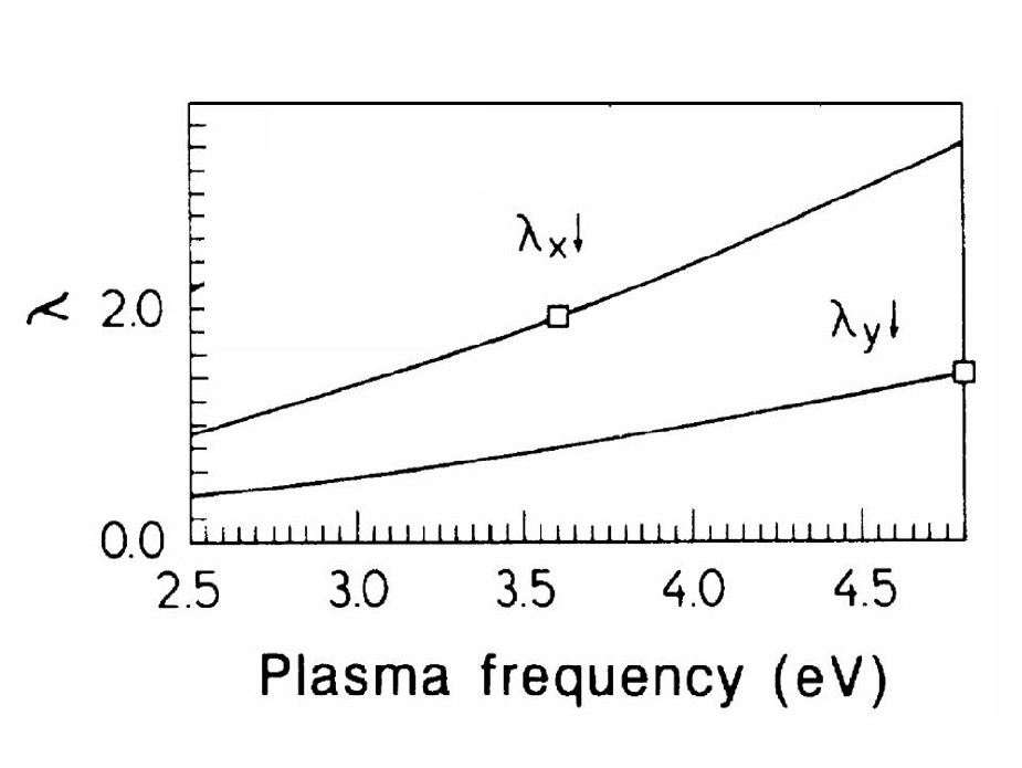
We shall argue below that from tunnelling experiments [23]-[28] one obtains in the framework of the Eliashberg theory that the EPI coupling constant is large which implies that , i.e. EPI is reduced in transport properties due to some reasons that shall be discussed in Part II. Such a large reduction of cannot be obtained within the LDA band structure calculations which means that and contain renormalization which do not enter in the theory. In Part II we shall argue that the strong suppression of may have its origin in strong electronic correlations and the long-range Madelung energy [45], [73].
4. Femtosecond time-resolved optical spectroscopy
The femtosecond time-resolved optical spectroscopy (FTROS) has been developed intensively in the last couple of years and applied successfully to HTSC cuprates. In this method a femtosecond () laser pump excites in materials electron-hole pairs via interband transitions. These hot carriers release their energy via electron-electron (with the relaxation time ) and electron-phonon scattering reaching states near the Fermi energy within - see [74]. The typical energy density of the laser pump pulses with the wavelength nm ( ) was around (the excitation fluenc ) which produces approximately carriers per puls (by assuming that each photon produces carriers, is the superconducting gap). By measuring photoinduced changes of the reflectivity in time, i.e. , one can extract information on the further relaxation dynamics of the low-laying electronic excitations. Since relax to equilibrium the fit with exponential functions is used
| (35) |
where ( is the Heavyside function) describes the finite rise-time. The parameters , depends on the fluenc . This method was used in studying the superconucting phase of , with , and and respectively [22]. In that case the signal for and for , while the signal was present also at . It turns out that the signal is related to the quasi-particle recombination across the superconducting gap and has a relaxation time of the order at . At the so called threshold fluenc ( for and for ) occurs the vaporization (destroying) of the superconducting phase, where the parameter saturates. This vaporization process takes place at the time scala . The external fluenc is distributed in the sample over the excitation volume which is proportional to the optical penetration depth ( at ) of the pump. The energy densities stored in the excitation volume at the vaporization threshold for and are and , respectively. The important fact is that is much larger than the superconducting condensation energy which is for and for , i.e. . This means that the energy difference must be stored elsewhere on the time scale . The only present reservoir which can absorb the difference in energy are the bosonic baths of phonons and spin fluctuations. The energy required to heat the spin reservoir from to is . The measured in [22] gives very small value . In the case of the phonon reservoir on obtains for and for . Since the spin reservoir cannot absorb the rest energy . The situation is opposite with phonons since and phonon can absorb the rest energy in the excitation volume. The complete vaporization dynamics can be described in the framework of the Rothwarf-Taylor model which describes approaching of electrons and phonons to quasi-equilibrium on the time scale of 1 ps [75]. We shall not go into details but only summarize, that only phonon-mediated vaporization is consistent with the experiments, thus ruling out spin-mediated quasi-particle recombination and pairing in HTSC cuprates. This is additional proof for the ineffectivness of the SFI scattering in cuprates.
In conclusion, optics and resistivity measurements in normal state of cuprates are much more in favor of EPI than against it. However, some intriguing questions still remain to be answered: (i) what are the values of and ; (ii) what is the reason that is realized in cuprates; (iii) what is the role of Coulomb scattering in and . Later on we shall argue that ARPES measurements in cuprates give evidence for a contribution of Coulomb scattering at higher frequencies, where for with . So, despite the fact that EPI is suppressed in transport properties it can be sufficiently strong in the self-energy in some frequency and temperature range.
III.3 ARPES and the EPI self-energy
ARPES is nowadays a leading spectroscopy method in the solid state physics [11]. It provides direct information to the one-electron removal spectrum in a complex many system. The method involves shining light (photons) with energies between on the sample and by detecting momentum () - and energy()-distribution of the outgoing electrons. The resolution of ARPES has been significantly increased in the last decade with the energy resolution of (for photon energies ) and angular resolution of . The ARPES method is surface sensitive technique, since the average escape depth () of the outgoing electrons is of the order of Å, depending on the energy of incoming photons. Therefore, very good surfaces are needed in order that the results be representative for bulk samples. The most reliable studies were done on the bilayer () and its single layer counterpart (), since these materials contain weakly coupled planes with the longest inter-plane separation in the cuprates. This results in a natural cleavage plane making these materials superior to others in ARPES experiments. After a drastic improvement of sample quality in other families of HTSC materials, the ARPES technique has became a central method in theoretical considerations. Potentially, it gives valuable information on the quasi-particle Green’s function, i.e. on the quasi-particle spectrum and life-time effects. The ARPES can indirectly give information on the momentum and energy dependence of the pairing potential. Furthermore, the electronic spectrum of the (above mentioned) cuprates is highly quasi-2D which allows an unambiguous determination of the initial state momentum from the measured final state momentum, since the component parallel to the surface is conserved in photoemission. In this case, the ARPES probes (under some favorable conditions) directly the single particle spectral function . In the following we discuss only those ARPES experiments which give evidence for the importance of the EPI in cuprates - see more in [11].
The photoemission measures a nonlinear response function of the electron system, and under some conditions it is analyzed in the so-called three-step model, where the total photoemission intensity is the product of three independent terms: (1) - describes optical excitation of the electron in the bulk; (2) - describes the scattering probability of the travelling electrons; (2) - the transmission probability through the surface potential barrier. The central quantity in the three-step model is and it turns out that it can be written in the form (for ) [11] with and the quasi-particle spectral function Im
| (36) |
Here, is the dipole matrix element which depends on , polarization and energy of the incoming photons. The knowledge of the matrix element is of a great importance and its calculation from first principles was done carefully in [76]. is the Fermi function, and are the quasi-particle Green’s function and the self-energy, respectively.
We summarize and comment here on some important ARPES results which were obtained recently and which confirm the existence of the Fermi surface and importance of EPI in quasi-particle scattering [11].
ARPES in the normal state
() There is a well defined Fermi surface in the metallic state with the topology predicted by the LDA. However, the bands are narrower than LDA predicts which points to a strong quasi-particle renormalization. () The spectral lines are broad with Im (or for ) which tells us that the quasi-particle liquid is a non-canonical Fermi liquid. () There is a bilayer band splitting in (at least in the over-doped state). The previous experiments did not show this splitting and served for various speculations on some exotic non-Fermi liquid scenarios. () At temperatures and in the under-doped cuprates there is a d-wave like pseudogap in the quasi-particle spectrum where increases by lowering doping. We stress that the pseudogap phenomenon is not well understood at present and we shall discuss this problem in Part II. Its origin can be due to a precursor superconductivity or due to a competing order, such as spin- or charge-density wave or something similar. () The ARPES self-energy gives clear evidence that EPI interaction is rather strong. For instance, at there are kinks in the quasi-particle dispersion in the nodal direction (along the line) at the characteristic phonon energy [48], see Fig. 13, and near the anti-nodal point at [77] - see Fig. 13.


That these kinks exist also above excludes the scenario with the magnetic resonance peak in . Since the magnetic neutron scattering give small SFI coupling constant . The kinks cannot be due to SFI as we already discussed above. () The position of the nodal kink is practically doping independent which points towards phonons as the scattering (gluing) boson. () The quasi-particles (holes) couple practically to the whole spectrum of phonons since at least three group of phonons were extracted from the ARPES effective self-energy in [78] - Fig. 14.

This result is in a qualitative agreement with numerous tunnelling measurements [23]-[28] which apparently demonstrate that the broad spectrum of phonons couples with holes without preferring any particular phonons - see discussion below. () Recent ARPES measurements in B2212 [49] show very different slope of the quasi-particle energy at very small and large energies - see Fig. 15. The theoretical analysis [79] of these results gives the total coupling constant , the EPI one while the Coulomb scattering (SFI is a part of it) is [79] - see Fig. 15. To this end let us mention some confusion related to the value of the EPI coupling constant extracted from ARPES. Namely, in [11], [80], [81] the EPI self-energy was obtained by subtracting the high energy slope of the quasi-particle spectrum at . The latter is apparently due to the Coulomb interaction. Although the position of the low-energy kink is not affected by this procedure (if ), the above (subtraction) procedure gives in fact an effective EPI self-energy and the coupling constant only. The latter is smaller than the real EPI coupling constant . The total self-energy is where is the contribution due to the Coulomb interaction. At very low energies one has usually , where is the characteristic Coulomb energies and the Coulomb coupling constant. The quasi-particle spectrum is determined from the condition
| (37) |
where is the bare band structure energy. At low energies , Eq.(37) can be rewritten in the form
| (38) |
| (39) |
| (40) |
Since at very low energies , one has and , then the real coupling constant is related to the effective one by
At higher energies , which are less important for pairing, the EPI effects are suppressed and stops growing, one has . The measured at near and slightly away from the nodal point in the optimally doped Bi2212 with [83] is shown in Fig. 15.

It is seen that has two kinks - the first one at low energy which is most probably of the phononic origin [11], [80], [81], while the second kink at higher energy is probably due to the Coulomb interaction. However, the important results in Ref. [83] is that the slopes of at low () and high energies () are different. The low-energy and high-energy slope near the nodal point are depicted and shown in Fig. 15 schematically (thin lines). From Fig. 15 it is obvious that EPI prevails at low energies . More precisely digitalization of in the interval gives the Coulomb coupling while the same procedure at gives the total coupling constant and the EPI coupling constant , i.e. the EPI coupling is at least twice larger than in the previous analysis of ARPES results. This estimation tells us that at (and near) the nodal point, the EPI interaction dominates in the quasi-particle scattering at low energies since , while at large energies (compared to ), the Coulomb interaction with dominates. We point out that EPI near the anti-nodal point can be even larger than in the nodal point, mostly due to the higher density of states near the anti-nodal point. () Recent ARPES spectra in the optimally doped near the nodal and anti-nodal point [81] show a pronounced isotope effect in , thus pointing to the important role of EPI - see more in the part related to the isotope effect. The isotope effect in can be well described in the framework of the Migdal-Eliashberg theory for EPI [82] as it will be discussed in Part II. () ARPES experiments on give strong evidence for the formation of small polarons in undoped cuprates which can be only due to phonons and strong EPI, while by doping quasi-particles appear and there are no small polarons [84]. Thus in [84], it a broad peak (around ) is observed at the top of the band () with the dispersion similar to that predicted by the model - see Fig. 16.

However, the peak in Fig. 16 is of Gaussian shape and can be described only by coupling to bosons, i.e. this peak is a boson side band - see more in [5] and references therein. The theory based on the t-J model (in the antiferromagnetic state of the undoped compound) by including coupling to several (half-breathing, apical oxygen, low-lying) phonons, which is given in [85], explains successfully this broad peak of the boson side band by the formation of small polarons due to the EPI coupling (). Note that this is for the polaron at the bottom of the band while in the case whwn the Fermi surface exists this coupling is even larger [85]. In [85] it was stressed that even when the electron-magnon interaction is stronger than the EPI one, the polarons are formed due to EPI. The latter involves excitation of many phonons at the lattice site (where the hole is seating), while it is possible to excite only one magnon at the given site.
() Recent soft x-ray ARPES measurements on the electron doped HTSC [86], and ( ), , [87] show kink at energies in the quasi-particle dispersion relation along both nodal and antinodal directions as it is shown in Fig. 17.

It is seen from this figure that the effective EPI coupling constant is isotropic and . The kink in the electron-doped cuprates is due solely to EPI and in that respect the situation is similar to the one in the hole-doped cuparates.
ARPES results in the superconducting state
() There is an anisotropic superconducting gap in most HTSC compounds [11], which is predominately d-wave like, i.e. with . () The kink at in the quasi-particle energy around the nodal point is not-shifted in the superconducting state while the antinodal kink at is shifted in the superconducting state by , i.e. [11]. To remind the reader, in the standard Eliashberg theory the kink in the normal state at should be shifted in the superconducting state to at any point at the Fermi surface. This puzzling result might be a smoking gun result since it makes a constraint on the quasi-particle interaction in cuprates. Until now there is only one plausible explanation [88] of this shift-non-shift puzzle which is based on an assumption of the forward scattering peak (FSP) in EPI - see more in Part II. The FSP in EPI means that electrons scatter into a narrow region around the starting point in the k-space, so that at the most part of the Fermi surface, there is weak (or no) mixing of states with different signs of the order parameter . () The recent ARPES spectra [89] on an undoped single crystalline 4-layered cuprate with apical fluorine (F), (F0234) gives strong evidence against SFI - see Fig. 18.

Namely, F0234 is not a Mott insulator - as expected from valence charge counting which puts valence as , but it is a superconductor with . Moreover, the ARPES data [89] reveal at least two metallic Fermi-surface sheets with corresponding volumes equally below and above half-filling - see Fig. 19.

One of the Fermi-surfaces is due to the electron-like () band (with % electron-doping) and the other one due to the hole-like () band (with hole-doping) and their split along the nodal direction is significant and cannot be explained by the LDA (or DFA) method [90]. This electron and hole self-doping of inner and outer layers is in an appreciable contrast to other multilayered cuprates where there is only hole self-doping. For instance, in HgBa2CanCun+1O2n+2 () and (Cu,C)Ba2CanCun+1O3n+2 (), the inner CuO2 layers are less hole-doped than outer layers. It turns out, unexpectedly, that the superconducting gap on the -band Fermi-surface is significantly larger than on the -one, i.e. their ratio is anomalous and is an order of magnitude larger than in the electron-doped cuprate . Furthermore, the -band Fermi-surface is rather far from the antinodal point at (). This is an extremely important result which means that the antiferromagnetic spin fluctuations with the AF wave-vector , as well as the van Hove singularity, are not important for the pairing in the -band. To remind the reader, the SFI scenario assumes that the pairing is due to spin fluctuations with the wave-vector which connects two anti-nodal points which are near the van Hove singularity at the hole-surface (at () and ()) giving rise to large density of states. This is apparently not the case for the -band Fermi-surface - see Fig. 19. The ARPES data give further that there is a kink at in the quasi-particle dispersion of both bands, while the kink in the -band is stronger than that in the -band. This result, together with the anomalous ratio , strongly disfavors SFI as a pairing mechanism.
() Despite the presence of significant elastic scattering in optimally doped Bi-2212, there are dramatic sharpening of the spectral function near the anti-nodal point at [91]. This can be explained by assuming that the small q-scattering (the forward scattering peak) dominates in the elastic impurity scattering [92], [93]. As a result, one finds that the impurity scattering rate in the superconducting state is almost zero, i.e. for for any kind of pairing (s- p- d-wave etc.) since the normal () and the anomalous () scattering rates compensate each other - the collapse of the elastic scattering rate. This result is a consequence of the Anderson-like theorem for unconventional superconductors which is due to the dominance of the small q-scattering [92]-[93]. In such a case d-wave pairing is weakly unaffected by impurities - there is small reduction in [93], [94]. The physics behind this result is rather simple. The small q-scattering (forward scattering) means that electrons scatter into a small region in the k-space, so that at the most part of the Fermi surface there is no mixing of states with different signs of the order parameter , and the detrimental effect of impurities is reduced. For states near the nodal points, there is mixing but since is small in this region, there is only small reduction in [42]. This result points to the importance of strong correlations in the renormalization of the impurity scattering - see discussion in Part II.
In conclusion, in order to explain ARPES results in cuprates it is necessary to take into account: (1) EPI interaction since it dominates in the quasiparticle scattering in the energy region responsible for pairing; (2) effects of elastic nonmagnetic impurities with FSP; (3) the Coulomb interaction which dominates at higher energies . In this respect, the presence of ARPES kinks and the knee-like shape of the spectral width are serious constraints for the pairing theory.
III.4 Tunnelling spectroscopy and spectral function
By measuring current-voltage characteristics in (normal metal-insulator-superconductor) tunnelling junctions with large tunnelling barrier - see more below, one obtains from tunnelling conductance the so called tunnelling density of states in superconductors . Moreover, by measuring of at voltages it is possible to determine the Eliashberg spectral function and finally to confirm (definitely) the phonon mechanism of pairing in materials, except heavy fermions. Four tunnelling techniques were used in the study of cuprates: vacuum tunneling by using the technique - scanning tunnelling microscope; point-contact tunnelling; break-junction tunnelling; planar-junction tunnelling. Each of these techniques has some advantages although in principle the most potential one is the STM technique [95]. It should be stressed that there are still difficulties in understanding tunnelling experiments in cuprates because of non-ideal tunnelling behavior of contacts [95]. Since tunnelling measurements probe a surface region of the order of superconducting coherence length , then this kind of measurements in materials with small coherence length ( Å in the plane and Å along the ) depends strongly on the surface quality and sample preparation. Nowadays, many of these material problems in cuprates are understood and as a result consistent picture of tunnelling features is starting to emerge.
From tunnelling experiments one obtains the energy gap in the superconducting state. Since we have already discussed this problem in [2], we will only briefly mention some important result, that in most cases, has V-shape in all families of HTSC hole and electron doped cuprates. This is due to pairing with the gapless spectrum, which is definitely confirmed in the interference experiments on hole and electron doped cuprates [41]. Some experiments give the U-shape of which resembles s-wave pairing. This controversy is explained to be the property of the tunneling matrix element which filters out states with the maximal gap.
Here we are interested in the electron-boson spectral function in HTSC cuprates which can be extracted by using tunnelling spectroscopy. We inform the reader in advance, that the shape and the energy width of , which are extracted from the second derivative at voltages above the superconducting gap, in most HTSC cuprates resembles the phonon density of states . This result is strong evidence for the importance of in the pairing potential of cuprates. For instance, plenty of break-junctions made from single crystals [23] show that the negative peaks in coincide with the peaks in the generalized phonon density of states measured by neutron scattering - see Fig. 20.

The tunnelling spectra in Bi2212 break junctions [23], which are shown in Fig. 20, indicates that the spectral function is unchanged in magnetic field which disfavors SFI since in the latter case, this function should be sensitive to the magnetic field. The reported broadening of the peaks in are partly due to the gapless spectrum of pairing in cuprates. Additionally, the tunnelling density of states at very low show a pronounced gap structure and it was found that , where and is some average value of the gap. In order to obtain the inverse procedure wasused by assuming superconductivity and the effective Coulomb parameter [23]. The obtained gives large coupling constant . Although this analysis [23] was done in terms of pairing, it mimics qualitatively the case of pairing, since one expects that pairing does not change significantly the global structure of at albeit introducing a broadening in it - see the physical meaning in Appendix A. We point out that the results obtained in [23] were reproducible on more than 30 junctions. In that respect very important results on slightly overdoped and on planar tunnelling junctions are obtained in [24] - see Fig. 21.

These results show very similar features to those obtained in [23] on break-junctions. It is worth mentioning that several
groups [25], [26], [27] have obtained similar
results for the shape of the spectral function from
the measurements on various cuprates - see the comparison in
Fig. 22. The latter results leave no much doubts about the
importance of the in pairing mechanism of cuprates.

In that respect tunnelling measurements on slightly overdoped [24], [28] are impressive, since the Eliashberg spectral function was extracted from the measurements of and by solving the inverse problem. The extracted has several peaks in broad energy region up to as it is seen in Fig. 21- 22, which coincide rather well with the peaks in the phonon density of states . In [28] numerous peaks, from , in are discerned as shown in Fig.24, which correspond to various groups of phonon modes - laying in (and around) these peaks. Moreover, in [24], [28] are extracted the coupling constants for these modes and their contribution () to as it is seen in Fig. 23. Note, due to the nonlinearity of the problem, the sum of is not equal to .

The next remarkable result is that the extracted coupling constant is very large,i.e. - see Fig. 23. It is obvious from Figs. (23-24) that almost all phonon modes contribute to and , which means that on the average, each particular phonon mode is not too strongly coupled to electrons thus keeping the lattice stable. None of the modes has too large , thus keeping the lattice stability.

For a better understanding of the the EPI coupling in these systems we show in Fig. 25 the total and partial density of phononic states.

In Fig. 23 it is seen that lower frequency modes from , corresponding to and vibrations, are rather strongly coupled to electrons (with ) and give appreciable contributions to . It is also seen in Fig. 23 that the coupling constants of the high-energy phonons ( with ) have and give moderate contribution to - around 10 %. These results confirm the importance of modes which cause the change of the Madelung energy in the ionic-metallic structure of HTSC cuprates, the idea also conveyed in [1], [2] - see more in Part II. If definitely confirmed, these results are in accordance with the moderate oxygen isotope effect in cuprates near the optimal doping. We stress that each peak in corresponds to many modes. In order to get filling on the structure of vibrations possibly strongly involved in pairing, we show in Figs. 26-27 the structure of these vibrations at special points in the Brillouin zone. It is seen in Fig. 26 that the low-frequency phonons are dominated by Cu, Sr, Ca vibrations.


It is seen in Fig. 23 that modes are stronger coupled to electrons than ones, although the density of state for the modes is larger. The reason for such an anomalous behavior might be due to symmetries of corresponding phonons as it is shown in Fig. 27. Namely to the peak contribute axial vibrations of O(1) in the Cu2 plane which are odd under inversion, while in the peak these modes are even. The in-plane modes of Ca and O(1) are present in which are in-phase and out-of-phase modes, while in they are all out-of-phase modes. For more information on other modes see [28]. We stress that the Eliashberg equations based on the extracted of the slightly overdoped with the ratio describe rather well numerous optical, transport and thermodynamic properties [28]. However, in underdoped systems with , where the pseudogap phenomena are pronounced, there are serious disagreements between experiments and the Eliashberg-like theory.
Similar conclusion, regarding the properties of the spectral function in cuprates, comes out from tunneling measurements on the Andreev ( low barrier)- and Giaver (, high barrier) -type junctions in and compounds [97], where the extracted is in accordance with the phonon density of states see Fig. 28.

Note that the BTK parameter is related to the transmission and reflection coefficients for the normal metal and respectively.
Although most of the peaks in in cuprates coincide with the peaks in the phonon density of states it is legitimate to put the question - can the magnetic resonance in the superconducting state give contribution to the ? In that respect very important inelastic neutron scattering measurements of the magnetic resonance as a function of doping [98] give that the resonance energy scales with , i.e. as shown in Fig.29.

This means that if one of the peaks in is due to the magnetic resonance at , then it shifts strongly with doping as it is observed in [98]. This is contrary to phonon peaks (energies) whose positions are doping independent. To this end, recent tunnelling experiments on Bi2212 [29] show clear doping independence of as it is seen in Fig. 30. This remarkable result is an additional and strong evidence in favor of EPI and against the SFI mechanism of pairing in HTSC cuprates.

It is interesting that in the vacuum tunneling measurements [99] the fine structure in at was not seen below , while the pseudogap structure is observed at temperatures near and above . This result could mean that the tunnelling is likely dominated by the nontrivial structure of the tunnelling matrix element (along the -axis), which is derived from the band structure calculations [100]. However, recent experiments on [30] give important information on possible nature of the bosonic mode which couples with electrons. In [30] the local conductance is measured where it is found that has peak at where has the maximal slope - see Fig. 31(a).


It turns out that the average phonon energy depends on the oxygen mass, i.e. , with and - as it is seen in Fig. 31(b). This result is a convincing evidence that phonons are strongly involved in the quasi-particle scattering. A possible explanation is put forward in [30] by assuming that this isotope effect is due to the B1g phonon which interacts with anti-nodal quasi-particles.
In our opinion the important message of tunnelling experiments in cuprates (by including too [101], [102]) is that there is strong evidence for the importance of EPI and that no particular phonon mode can be singled out in the spectral function as being the only one which dominates in pairing mechanism. This important result means that the high is not attributable to a particular phonon mode in the mechanism, i.e. all phonon modes contribute to . Having in mind that the phonon spectrum in cuprates is very broad (up to ), then the large constant () obtained in tunnelling experiments is not surprising at all.
III.5 Phonon spectra and EPI
Although experiments, such as inelastic neutron and Raman scattering, related to phonon spectra and their renormalization by do not give directly , as the tunnelling and optic spectra do, they nevertheless give useful information on the strength of EPI for some particular phonons. We stress in advance that the interpretation of experimental results in terms of EPI for weakly interacting electrons might be risky since in strongly correlated systems, such as HTSC cuprates, the phonon renormalization due to EPI is rather different from that in weakly correlated metals - see [103]. Since these questions are thoroughly studied in the excellent review [103] - see also Part II, we shall briefly enumerate the main points: (1) In strongly correlated systems, the EPI coupling for a number of phononic modes can be significantly larger than the LDA and Hartree-Fock methods predict. This is due to many-body effects [103]. (2) In strongly correlated systems the quasi-particle charge susceptibility, which enters the phonon self-energy , is much more suppressed than in weakly correlated metals and these effects are out of the LDA possibilities [2], [104], [103]. This is one of the reasons that the analysis of experiments on phonon renormalizations in the framework of LDA underestimates the EPI coupling constant significantly - on all these questions, see more details in Part II.
III.5.1 The phonon Raman scattering
The phonon Raman scattering gives also evidence for appreciable EPI in cuprates [111], [112], [113]. We enumerate some of them - see more in [2] and References therein. (i) There is a pronounced asymmetric line-shape (of the Fano resonance) in the metallic state. For instance, in two Raman modes at (Ba dominated mode) and at (O dominated mode in the CuO2 planes) show pronounced asymmetry which is absent in . This result points to appreciable interaction of Raman active phonons with continuum states (quasi-particles) [111], [112],. (ii) The phonon frequencies for some and are strongly renormalized in the superconducting state, between , pointing again to large EPI [113] - see also in [2], [44]. To this point we mention that the electronic Raman scattering in cuprates show a remarkable correlation between the Raman cross-section and the optical conductivity in the a-b plane , i.e. [2]. It was argued above that EPI with the very broad spectral function explains in a natural way the and dependence of . This means that the electronic Raman spectra in cuprates can be explained by EPI in conjunction with strong correlations. This conclusion is supported by calculations of the Raman cross-section [105] which take into account EPI with extracted from tunnelling measurements in and [2], [23]-[28]. Quite similar properties (to cuprates) of the electronic Raman scattering, as well as of , and , were observed in experiments [62] on isotropic 3D metallic oxides and where there are no signs of antiferromagnetic fluctuations. This means that low-dimensionality and antiferromagnetic spin fluctuations cannot be a prerequisite for anomalous scattering of quasi-particles and EPI must be inevitably taken into account since it is present in all these compounds.
III.5.2 Neutron scattering, phonon spectra and EPI
The softening of numerous phonon modes has been observed in the normal state of cuprates giving important evidence for pronounced EPI. There are several important reviews on this subject [108] and here we discuss briefly two important examples which demonstrate in an impressive way the inefficiency of the LDA band structure calculations to treat quantitatively and qualitatively EPI in HTSC cuprates. Namely, by doping the Cu-O bond-stretching phonon mode shows a substantial softening at - called the half-breathing phonon, and a large broadening by 5 meV at 15% doping. While the softening can be partly described by the LDA method [109], it predicts an order of magnitude smaller broadening than the experimental one. The reason for this failure lies in strong correlations, which are not included in the LDA method as explained in [2], [5], [104], [103]. They give rise to an increase of the EPI coupling and to strong suppression of the charge fluctuations which enter the phonon self-energy via the charge susceptibility - see below and in Part II. The neutron scattering in gives evidence for large (30%) softening of the O with symmetry with the energy , which is theoretically predicted in [106], and for the large line-width about 17 meV which also suggest strong EPI.
As it is discussed in the Introduction, there are recently several calculations of the EPI coupling constant in the framework of DFT (or LDA), where very small was obtained [13], [14]. However, the LDA method is inadequate for strongly correlated systems as it does not correctly take into account exchange-correlations and many-body effects, and therefore overestimates the screening in cuprates. If DFT is able to describe EPI correctly, it must also be able to calculate phonon renormalization, such as softening and broadening of the spectrum. In fact DFT completely fails to describe this renormalization for some important phonon modes and therefore fails to describe the effect of EPI on the electronic spectrum. The critique of LDA (DFT) results in HTSC cuprates is done in [2] and recently strongly argued in [5], [110] by its disagreement with neutron scattering measurements as it is shown in Fig. 32.

The point is that DFT (LDA) can reproduce the phonon softening in and rather good at low momenta but predicts smooth softening at higher , while experiments show pronounced features for . At the same time DFT predicts an order of magnitude smaller line width than experiments [114].
In Part II we shall discuss some theoretical approaches related to EPI renormalization of phonons in strongly correlated systems. Here, we point out two results. First, there is an appreciable difference in the phonon renormalization in strongly and weakly correlated systems. Namely, the change of phonon frequencies in the presence of conduction electrons is proportional to the coupling constant and charge susceptibility , i.e. , while the line width is given by . It turns out that in strongly correlated systems doped with hole concentration the charge fluctuations are suppressed in which case the following sum-rule holds [5], [104]
while in the LDA method one has
This means that for low doping (note ), one has and LDA strongly underestimates the coupling constant, i.e. . We stress that there is no such strong suppression in the quasi-particle self-energy [5].
Second, the theory gives that the coupling constant in HTSC cuprates can be significantly larger than LDA predicts, which is due to some many-body effects not present in the latter [5], [104]. It can be shown that for some phonon modes one has . For instance, for the half-breathing mode, one has that is first calculated in [104]. These results point to inadequacy of LDA in calculations of EPI effects in HTSC cuprates.
III.6 Isotope effect for various doping
The isotope effect in the critical temperature was one of the very important proof for the EPI pairing in low-temperature superconductors (LTSC). As a curiosity the isotope effect in systems was measured almost exclusively in monoatomic systems and in few polyatomic systems: the hydrogen isotope effect in , the and isotope shift of in , and the isotope effect in and . We point out that very small ( in and ) and even negative (in ) isotope effect in some polyatomic systems of materials are compatible with the pairing mechanism but in the presence of substantial Coulomb interaction or lattice anharmonicity. The isotope effect cannot be considered as the smoking gun since it is sensitive to numerous influences. For instance, in it is with certainty proved that the pairing is due to EPI and strongly dominated by the boron vibrations, but the boron isotope effect is significantly reduced, i.e. . It is still unexplained. The situation in HTSC cuprates is much more complicated because they contain many-atoms in unit cell. Additionally, the situation is complicated with the presence of intrinsic and extrinsic inhomogeneities which can mask real effects. On the other hand new techniques such as ARPES, STM, allow studies of the isotope effects in quasi-particle self-energies, i.e. , which will be discussed below.
III.6.1 Isotope effect in
This problem will be discussed only briefly since more extensive discussion can be found in [2]. It is well known that in the pure EPI pairing mechanism, the total isotope coefficient is given by
| (41) |
where is the mass of the i-th element in the p-th crystallographic position. Note that in the case when the screened Coulomb interaction is negligible, i.e. , one has . From this formula one can deduce that the relative change of , , for heavier elements is rather small - for instance it is 0.02 for , 0.03 for and 0.07 for . This means that measurements of for heavier elements are at/or beyond the ability of present day experimental techniques. Therefore most isotope effect measurements were done by substituting light atoms by only. It turns out that in most optimally doped HTSC cuprates is small. For instance in with , but it is appreciable in with where. In with one has while and even negative () in with . The experiments on () with are still unreliable and is unknown: In the electron-doped with one has while in the underdoped materials increases. The largest is obtained even in the optimally doped compounds like in systems with substitution, such as , , where for . In there is a isotope effect which is of the order of the oxygen one, i.e. giving for optimally doped systems (). In case when with one has with [107]. The appreciation of copper isotope effect in tells us that vibrations other than oxygen ions are important in giving high Tc. In that sense one should have in mind the tunnelling experiments discussed above, which tell us that all phonons contribute to the Eliashberg pairing function and according to these results the oxygen modes give moderate contribution to [28]. Having these facts in mind, then the small oxygen isotope effect in optimally doped cuprates, if it is intrinsic property, does not exclude the EPI mechanism of pairing.
III.6.2 Isotope effect in the self-energy
The fine structure of the quasi-particle self-energy , such as kinks, can be resolved in ARPES measurements and in some respect in STM. It turns out that there is an isotope effect in the self-energy in the optimally doped samples [81], [115], [116]. In the first paper on this subject [81], there is a red shift of the nodal kink at for the substitution. This isotope shift of the self-energy is more pronounced at large energies . However, there is a dispute on the latter result which is not confirmed experimentally [115], [116]. The isotope effect in [115], [116] can be well described in the framework of the Migdal-Eliashberg theory for EPI [82] which is in accordance with the recent ARPES measurements with low-energy photons [117]. The latter allowed very good precision in measuring the isotope effect in the nodal point of Bi2212 with and [117]. They observed shift in the maximum of Re - at which corresponds to the half-breathing or breathing phonon, by as shown in Fig. 33.

By analyzing the shift in Im - shown in Fig. 33, one finds similar result . The similar shift was obtained in STM measurements [30] which is shown in Fig. 31(b) and can have its origin in different phonons. We would like to stress two points: (i) in compounds with the isotope effect in is moderate, i.e. , [117]. If we consider this value to be intrinsic then it is not in conflict with the tunnelling experiments in [28] which give evidence that vibrations of heavier ions contribute significantly to - see the above discussion on the tunnelling spectroscopy; (ii) the extracted value in [117] of the effective EPI coupling constant , which is smaller than the real - see above the discussion on ARPES, is significantly larger than the LDA theory predicts [13], [14]. This again points that the LDA method does not pick up the many-body effects due to strong correlations- see Part II.
IV Summary of Part I
The analysis of experimental data in HTSC cuprates which are related to optics, tunnelling and ARPES measurements near the optimal doping give evidence for the large electron-phonon interaction with the coupling constant . The analysis is done in the framework of the Migdal-Eliashberg theory which is a reliable approach for systems near the optimal doping. The spectral function averaged over the Fermi surface is extracted from various tunnelling measurements and it contains peaks at the same positions as the phonon density of states. The energy width of is the same as the width of the phonon density of states . This is an unambiguous proof for the important role which EPI plays in the pairing mechanism of cuprates. The optical IR reflectivity data provide additional support for this finding since the transport spectral function has the width and global properties similar to . These findings are additionally and strongly supported by ARPES measurements on BISCO compounds. The ARPES kinks in the quasi-particle self-energy can be explained exclusively by EPI and there is no much room for spin fluctuations (SFI) effects. The weakness of SFI is unambiguously proved in magnetic neutron scattering on YBCO where the imaginary part of the susceptibility is drastically reduced in the low energy region by going from slightly underdoped toward optimally doped systems, while is practically unchanged. This implies that the SFI coupling constant is limited to the value . All these results do not leave doubts on the significance of EPI and weakness of SFI. The obtained total EPI coupling constant is rather large, i.e. , while the transport coupling constant is . The different renormalization of the quasi-particle and transport self-energies by the Coulomb interaction and strong correlations points to dominance of the small-momentum scattering in EPI. This will be discussed in Part II.
Inelastic neutron scattering measurements in cuprates show that the broadening of phonon lines is by an order of magnitude larger than the LDA (DFA) method predicts. Since the phonon line-widths depend on the EPI coupling and the charge susceptibility it is evident that calculations of both quantities are beyond the range of applicability of LDA. As a consequence, LDA overestimates electronic screening and thus underestimates the EPI coupling. This means that LDA is suitable only for weakly correlated systems, while many-body effects due to strong correlations are not contained in this mean-field type theory.
In spite of the very promising and encouraging results about the dominance of EPI in cuprates the theory is still confronted with the task of obtaining sufficiently large coupling constant in the d-channel in order that EPI conforms with d-wave pairing. At present we do not have such a detailed microscopic theory although some concepts, such as the the dominant EPI scattering at small transfer momenta, are understood at least qualitatively. These set of problems and questions will be discussed in Part II.
Acknowledgement. We are thankful to Vitalii Lazarevich Ginzburg for his permanent interest in our work and for support in many respects over many years. One of us (M. L. K.) is thankful to Karl Bennemann for inspiring discussions on many subjects related to physics of HTSC cuprates. We thank Godfrey Akpojotor for careful reading of the manuscript. M. L. K. is thankful to the Max-Born-Institut für Nichtlineare Optik und Kurzzeitspektroskopie, Berlin for the hospitality and financial support during his stay where part of this work has been done.
V Appendix - Spectral functions
V.1 Spectral functions and
Before discussing experimental results in cuprate superconductors which are related to various spectral functions, we introduce the reader briefly into the subject. The quasiparticle-bosonic (Eliashberg) spectral function and its Fermi surface average enter the quasi-particle self-energy , while the transport spectral function enters the transport self-energy and dynamical conductivity . Since the Migdal-Eliashberg theory for EPI is well defined we define the spectral functions for this case and the generalization to other electron-boson interaction is straightforward. In the superconducting state the Matsubara Green’s function and are matrices with the diagonal elements and off-diagonal elements which describe superconducting pairing. By defining and , the Eliashberg functions for EPI in the presence of the Coulomb interaction (in the pairing channel) read [118], [119], [120]
| (42) |
| (43) |
| (44) |
where is the density of states at the Fermi surface, , and . (For studies of optical properties - see below, it is useful to introduce the renormalized frequency (or its analytical continuation ). These equations are supplemented with the electron number equation ( is the chemical potential)
| (45) |
Note that in the case of EPI one has (with ) where is defined by
| (46) |
| (47) |
where is the phonon spectral function of the -th phonon mode related to the phonon propagator
| (48) |
The renormalized coupling constant comprises the screening effect due to long-range Coulomb interaction ( - the inverse electronic dielectric function) and short-range strong correlations ( - the vertex function) - see more in Part II. Usually in the case of low-temperature superconductors (LTS) with s-wave pairing the anisotropy is rather small (or in the presence of impurities it is averaged out) which allows an averaging of the Eliashberg equations [118], [119], [120]
| (49) |
| (50) |
| (51) |
Here where is the average over the Fermi surface. The above equations can be written on the real axis by the analytical continuation where the gap function is complex i.e. . The solution for allows the calculation of the current-voltage characteristic and tunnelling conductance in the superconducting state of the tunneling junction where is given by
| (52) |
Here, are the spectral functions of the normal metal and superconductor, respectively and is the Fermi distribution function. Since the angular and energy dependence of the tunnelling matrix elements is practically unimportant for superconductors, then in that case the relative conductance is proportional to the tunnelling density of states , i.e. where
| (53) |
Here, , , and the quasi-particle scattering rate in the superconducting state is given by
| (54) |
where is the quasi-particle density of states in the superconducting state, are Bose and Fermi distribution function respectively. Since the structure of phononic spectrum is contained in , it is reflected on for (the real gap obtained from ) which gives the structure in at . On the contrary one can extract the spectral function from by the inversion procedure proposed by McMillan and Rowell [121], [2]. It turns out that in low-temperature superconductors, negative peaks of at , correspond to the peak positions of and . However, we would like to point out that in HTSC cuprates the gap function is unconventional and very anisotropic, i.e. . Since in this case the extraction of is extremely difficult and at present rather unrealistic task, then an ”average” is extracted from the experimental curve . There is belief that it gives relevant information on the real spectral function such as the energy width of the bosonic spectrum () and positions and distributions of peaks due to bosons. It turns out that even such an approximate procedure gives valuable information in HTSC cuprates - see discussion in Section III D.
Note that in the case of spin-fluctuation interaction (the SFI model) one should make difference between and since they differ by sign i.e. since SFI is repulsive in the pairing-channel - see Eqs. (7-8).
V.1.1 Inversion of tunnelling data
Phonon features in the conductance at makes the tunnelling spectroscopy a powerful method in obtaining the Eliashberg spectral function . Two methods were used in the past for extracting .
The first method is based on solving the inverse problem of the nonlinear Eliashberg equations. Namely, by measuring , one obtains the tunnelling density of states and by the inversion procedure one gets [121]. In reality the method is based on the iteration procedure - the McMillan-Rowell () inversion, where in the first step an initial , and are inserted into Eliashberg equations (for instance for and for ) and then is calculated. In the second step the functional derivative () is found in the presence of a small change of and then the iterated solution is obtained, where the correction is given by
| (55) |
The procedure is iterated until and converge to and which reproduce the experimentally obtained conductance . In such a way the obtained for resembles the phonon density of states , that is obtained from neutron scattering measurements. Note that the method depends explicitly on but on the contary it requires only data on up to the voltage where is the maximum phonon energy ( for ) and is the zero-temperature superconducting gap. One pragmatical feature for the interpretation of tunnelling spectra (and for obtaining the spectral pairing function ) in and cuprates is that the negative peaks of are at the peak positions of and . This feature will be discussed later on in relation with experimental situation in cuprates.
The second method has been invented in [122] and it is based on the combination of the Eliashberg equations and dispersion relations for the Greens functions - we call it GDS method. First, the tunnelling density of states is extracted from the tunneling conductance in a more rigorous way [123]
| (56) |
where and the constant is obtained from at large biases - see [122]. under the integral can be replaced by the BCS density of states. Since the second method is used in extracting in a number of LTSC as well as in HTSC cuprates - see below, we describe it briefly for the case of isotropic EPI at T=0 K. In that case the Eliashberg equations are [118], [119], [120], [122]
| (57) |
| (58) |
where
| (59) |
Here is the Coulomb pseudopotential, the cutoff is approximately , is the energy gap. Now by using the dispersion relation for the matrix Greens functions one obtains [122]
| (60) |
where . From Eqs. (57-58) one obtains
| (61) |
V.1.2 Phonon effects in
We briefly discuss the physical origin for the phonon effects in by considering a model with only one peak, at , in the phonon density of states by assuming for simplicity and neglecting the weak structure in at , which is due to the nonlinear structure of the Eliashberg equations [125].

In Fig.34 it is seen that the real gap reaches a maximum at then decreases, becomes negative and zero, while is peaked slightly beyond that is the consequence of the effective electron-electron interaction via phonons.
It follows that for most phonons have higher energies than the energy of electronic charge fluctuations and there is over-screening of this charge by ions giving rise to attraction. For charge fluctuations are in resonance with ion vibrations giving rise to the peak in . For the ions move out of phase with respect to charge fluctuations giving rise to repulsion and negative . This is shown in Fig. 34(b). The structure in is reflected on as shown in Fig. 34(c) which can be reconstructed from the approximate formula for expanded in powers of
As increases above this gives , while for the real value decreases while rises and decreases giving rise for .
V.2 Transport spectral function
The spectral function enters the dynamical conductivity ( axis in systems) which generally speaking is a tensor quantity given by the following formula
| (62) |
where and and the bare current vertex is related to the Fermi velocity , i.e. The vertex function takes into account the renormalization due to all scattering processes responsible for finite conductivity [124]. In the following we study only the in-plane conductivity at . The latter case is realized due to the long penetration depth in HTSC cuprates and the skin depth in the normal state are very large. In the theory, is a solution of an approximative integral equation written in the symbolic form [68]
| (63) |
where the effective potential (due to EPI) is given by , where is the phonon Green’s function. In such a case the Kubo theory predicts ()
| (64) |
where , and is the impurity contribution. In the following we omit the tensor index in . In the presence of several bosonic scattering processes the transport self-energy is given by
| (65) |
| (66) |
| (67) |
Here is the transport spectral function which measures the strength of the -th (bosonic) scattering process and is the digamma function. The index enumerates EPI, charge and spin-fluctuation scattering processes. Like in the case of EPI, the transport bosonic spectral function is given explicitly by
| (68) |
We stress that in the phenomenological SFI theory [6] one assumes Im, which, as we have repeated several times, can be justified only for small , i.e. (the band width).
In case of weak coupling (), can be written in the generalized (extended) Drude form as discussed in Section III.B.
References
- [1] E. G. Maksimov, Uspekhi Fiz. Nauk 170, 1033 (2000); V. L. Ginzburg, E, G. Maksimov, Physica C 235-240, 193 (1994); Superconductivity (in Russian) 5, 1505 (1992)
- [2] M. L. Kulić, Phys. Reports 338, 1-264 (2000)
- [3] C. Falter, phys. stat. solidi (b) 242, 118 (2005)
- [4] A. S. Alexandrov, arXiv:0808.3520; T. M. Hardy, J. P. Hague, J. H. Samson, A. S. Alexandrov, arXiv:0806.2810
- [5] O. Gunnarsson, O. Rösch, J. Phys: Condens. Matter 20, 043201 (2008); O. Rösch, J. E. Hahn, O. Gunnarsson, V. H. Crespi, phys. stat. solidi (b) 242, 78 (2005)
- [6] A. J. Millis, H. Monien, D. Pines, Phys. Rev. B 42, 167 (1990); P. Monthoux and D. Pines, Phys. Rev. Lett. 69, 961 (1992); Phys. Rev. B 47, 6069 (1993); B. P. Stojković, D. Pines, Phys. Rev. B56, 11931 (1997); D. Pines, preprint CNSL Newsletter, LALP-97-010, No. 138, June 1997; Physica B163, 78 (1990)
- [7] P. A. Lee, N. Nagaosa, C.-G. Wen, Rev. Mod. Phys. 78, 17 (2006)
- [8] T. Ami, M. Imada, J. Phys. Soc. Jpn. 76, 113708 (2007)
- [9] D. J. Scalapino, S. R. White, S. C. Zhang, Phys. Rev. Lett. 68, 2830 (1992)
- [10] L. Pryadko, S. Kivelson, O. Zachar, Phys. Rev. Lett. 92, 067002 (2004)
- [11] A. Damascelli, Z. Hussain, Z. -X. Shen, Rev. Mod. Phys. 75, 473 (2003); J. C. Campuzano, M. R. Norman, M. Randeria, cond-mat/0209476 (2002)
- [12] J. Hwang et al., Phys. Rev. Lett. 100, 137005 (2008)
- [13] R. Heid et al., Phys. Rev. Lett. 100, 137001 (2008)
- [14] F. Giuistino et al., Nature 452, 975 (2008)
- [15] E. G. Maksimov, M. L. Kulić, O. V. Dolgov, G. Akpojotor, in preparation
- [16] Ph. Bourges, in The Gap Symmetry and Fluctuations in High Temperature Superconductors, J. Bok, G. Deutscher, D. Pavuna, S. A. Wolf, Eds. (Plenum, New York, 1998), pp. 349-371; preprint cond-mat/9901333 (1999)
- [17] P. B. Allen, Phys. Rev. B3, 305 (1971)
- [18] O. V. Dolgov, S. V. Shulga, J. of Superconductivity 8, 611 (1995); S. V. Shulga, O. V. Dolgov, E. G. Maksimov, Physica C178, 266 (1991), O. V. Dolgov, E. G. Maksimov, S. V. Shulga, in Electron-Phonon Interaction in Oxide Superconductors, ed. R. Baquero, World Scien., p.30 (1991)
- [19] S. V. Shulga, in High- Superconductors and Related Materials, p. 323 (2001), eds. S.-L. Drechsler, T. Mishonov, Kluwer Academic Publishers
- [20] A. E. Karakozov, E. G. Maksimov, O. V. Dolgov, Sol. St. Comm. 124, 119 (2002)
- [21] A. E. Karakozov, E. G. Maksimov, Solid St. Commun. 139, 80 (2006)
- [22] P. Kusar et al., arXiv: 0805.0536v2
- [23] L. N. Bulaevskii, O. V. Dolgov, I.P. Kazakov, S.N. Maksimovskii, M.O. Ptitsyn, V.A. Stepanov, S.I. Vedeneev, Supercond. Science Technology, 1, 205 (1988); S. I. Vedeneev, A. G. M. Jensen, P. Samuely, V. A. Stepanov, A. A. Tsvetkov and P. Wyder, Phys. Rev. 49, 9823 (1994); S. I. Vedeneev, A. G. M. Jansen, A. A. Tsvetkov, P. Wyder, Phys. Rev. B 51, 16380 (1995); S. I. Vedeneev, A. G. M. Jensen and P. Wyder, Physica B 218, 213 (1996)
- [24] D. Shimada, Y. Shiina, A. Mottate, Y. Ohyagi and N. Tsuda, Phys. Rev. B 51, 16495 (1995); N. Miyakawa, A. Nakamura, Y. Fujino, T. Kaneko, D. Shimada, Y. Shiina and N. Tsuda, Physica C 282-287, 1519 (1997);
- [25] N. Miyakawa, Y. Shiina, T. Kaneko and N. Tsuda, J. Phys. Soc. Jpn. 62, 2445 (1993); N. Miyakawa, Y. Shiina, T. Kido and N. Tsuda, J. Phys. Soc. Jpn. 58, 383 (1989)
- [26] Y. Shiina, D. Shimada, A. Mottate, Y. Ohyagi and N. Tsuda, J. Phys. Soc. Jpn. 64, 2577 (1995); Y. Ohyagi, D. Shimada, N. Miyakawa, A. Mottate, M. Ishinabe, K. Yamauchi and N. Tsuda, J. Phys. Soc. Jpn. 64, 3376 (1995)
- [27] R. S. Gonnelli, F. Asdente and D. Andoreone, Phys. Rev. B 49, 1480 (1994)
- [28] D. Shimada et al., Physica C 298, 195 (1998); N. Tsuda et al., in New Research on Superconductivity, Ed. Barry P. Martinis, pp. 105-141, 2007 Nova Science Publishers, Inc.
- [29] Y. G. Ponomarev et al., in Proc. of the Intern. Conf. on Strongly Correlated Systems, Houston, Texas, USA, May 13-17, 2007, p. 190; Physica C (2008)
- [30] K. McElroy, R. W. Simmonds, J. E. Hoffman, D. H. Lee, K. M. Lang, J. Orenstein, H. Eisaki, S. Uchida, J. C. Davis, Nature 422, 592 (2003); J. Lee et al., Bull. Am. Phys. Soc. 50, 299 (2005); J. C. Davis et al., Bull. Am. Phys. Soc. 50, 1223 (2005)
- [31] F. Marsiglio et al., Phys. Rev. B50, 7023 (1994)
- [32] O. Klein et al., Phys. Rev. B50, 6307 (1994)
- [33] D. G. Hinks, J. D. Jorgensen, Physica C385, 98 (2003)
- [34] J. C. Phillips, phys. stat. solidi (b) 242, 51 (2005)
- [35] M. L. Cohen, P. W. Anderson, Superconductivity in and band metals, AIP Conference Proceedings (ed. D. H. Douglass) New York, p.17 (1972); reprint in P.W. Anderson A Career in Theoretical Physics (World Scientific, 1994) p. 288
- [36] O. V. Dolgov, E. G. Maksimov, Uspekhi Fiz. Nauk 177, 983 (2007) ( Phys.-Uspekhi, 50, 933 (2007))
- [37] D. A. Kirzhnitz, in High Temperature Superconductivity, eds. V. L. Ginzburg and D. Kirzhnitz, Consultant Bureau New York, London, 1982; D. A. Kirzhnitz, Chapter 2 in: ”Dielectric Function of Condensed Systems”, eds. L.V.Keldysh, D.A.Kirzhnits, A.A.Maradudin, Elsevier Publ., Amsterdam (1989)
- [38] O. V. Dolgov, D. A. Kirzhnitz, E. G. Maksimov, Rev. Mod. Phys. 53, 81 (1981); O.V. Dolgov, D.A. Kirzhnits, E.G. Maksimov, Chapter 2 in: ”Superconductivity, Superdiamagnetism and Superfluidity”, ed. by V.L.Ginzburg, MIR Publ., Moscow (1987) (in English); O.V. Dolgov, E.G.Maksimov, Chapter 4 in: ”Dielectric Function of Condensed Systems”, eds. L.V.Keldysh, D.A.Kirzhnits, A.A.Maradudin, Elsevier Publ., Amsterdam (1989)
- [39] J. E. Moussa, M. L. Cohen, Phys. Rev. B 74, 094520 (2006)
- [40] P. W. Anderson, Science 316, 1705 (2007)
- [41] C. C. Tsuei, J. R. Kirtley, Rev. Mod. Phys. 72, 969 (2000)
- [42] A. I. Lichtenstein, M. L. Kulić, Physica C 245, 186 (1995)
- [43] D. J. Scalapino, Physics Reports 250, 329(1995)
- [44] M. L. Kulić, AIP Conference Proceedings Volume 715, 75 (2004), Lectures On The Physics Of Highly Correlated Electron Systems; M. L. Kulić, O. V. Dolgov, phys. stat. solidi (b) 242, 151 (2005)
- [45] M. L. Kulić, R. Zeyher, Phys. Rev. B 49, 4395 (1994); Physica C 199-200, 358 (1994); Physica C 235-240, 358 (1994)
- [46] H. Y. Kee, S. A. Kivelson, G. Aeppli, Phys. Rev. Lett. 88, 257002 (2002)
- [47] M. L. Kulić, I. M. Kulić, Physica 391, 42 (2003)
- [48] A. Lanzara et al., Nature 412, 510 (2001)
- [49] T. Valla et al., Science 285, 2110 (1999)
- [50] I. Božović, Phys. Rev. B 42, 1969 (1990)
- [51] Z. Schlesinger et al., Phys. Rev. Lett. 65, 801 (1990)
- [52] D. B. Romero et al., Phys. Rev. Lett. 68, 1590 (1992); D. B. Romero et al., Sol. St. Comm. 82, 183 (1992)
- [53] A. V. Puchkov, D. N. Basov, T. Timusk, J. Phys.: Condens. Matter 8, 10049 (1996); J. Hwang, T. Timusk, G. D. Gu, Nature 427, 714 (2004); M. Norman, Nature 427, 692 (2004).
- [54] F. Gao et all., Phys. Rev. B47, 1036 (1993)
- [55] A. V. Boris et al., Science 304, 708 (2004).
- [56] H. J. Kaufmann, Ph. D. Thesis, Uni. Cambridge, February 1999
- [57] J. Schutzmann et al., Phys. Rev. B46, 512 (1992)
- [58] K. Kamaras et al., Phys. Rev. Lett. 64, 84 (1990)
- [59] E. Schachinger, J. P. Carbotte, Phys. Rev. B 64, 094501 (2001)
- [60] J. Hwang et al., Phys. Rev. B75, 144508 (2007); J. Hwang et al., Nature (London) 427, 714 (2004)
- [61] B. Vignolle et al., Nature Phys. 3, 163 (2007)
- [62] I. Božović, J. H. Kim, J. S. Harris, Jr., C. B. Eom, J. M. Phillips, J. T. Cheung, Phys. Rev. Lett., 73, 1436 (1995)
- [63] J. E. Hirsch, Physica 201, 347 (1992)
- [64] P. F. Maldague, Phys. Rev. B16, 2437 (1977)
- [65] F. Carbone et al., Phys. Rev. B74, 024502 (2006); F. Carbone et al., Phys. Rev. B74, 064510 (2006)
- [66] H. J. Molegraaf et al., Science 295, 2239 (2002)
- [67] G. Deutscher et al., Phys. Rev. B72, 095504 (2005)
- [68] H. J. Kaufmann, E. G. Maksimov, E. K. H. Salje, J. of Supercond. 11, 755 (1998)
- [69] I. I. Mazin, O. V. Dolgov, Phys. Rev. B45, 2509 (1992)
- [70] T. A. Friedman et al., Phys. Rev. B42, 6217 (1990)
- [71] P. B. Allen, Nature 412, 494 (2001)
- [72] A. F. Santander-Syro eta al., Europhys. Lett. 62, 568 (2003)
- [73] R. Zeyher, M. L. Kulić, Phys. Rev. B53, 2850 (1996); R. Zeyher, M. L. Kulić, Phys. Rev. B54, 8985 (1996); M. L. Kulić and R. Zeyher, Mod. Phys. Lett. B 11, 333 (1997)
- [74] D. Mihailović, V. V. Kabanov, Struct Bond (2005) 114, p. 331-364, Springer-Verlag Berlin-Heidelberg 2005
- [75] V. V. Kabanov et al., Phys. Rev. Lett. 95, 147002 (2005)
- [76] A. Bansil, M. Lindros, Phys. Rev. Lett. 83, 5154 (1999)
- [77] T. Cuk et al., Phys. Rev. Lett. 93, 117003 (2004)
- [78] X. J. Zhou et al., Phys. Rev. Lett. 95, 117001 (2005)
- [79] M. L. Kulić, O. V. Dolgov, Phys. Rev. B 76, 132511 (2007)
- [80] T. Cuk et al., phys. stat. solidi (b) 242, 11 (2005)
- [81] G.-H. Gweon et al., Nature 430, 187 (2004)
- [82] E. G. Maksimov, O. V. Dolgov, M. L. Kulic, Phys. Rev. B72, 212505 (2005)
- [83] T. Valla, T. E. Kidd, Z.-H. Pan, A. V. Fedorov, W.-G. Yin, G. D. Gu, P. D. Johnson, Phys. Rev. Lett. 98, 167003 (2007)
- [84] K. M. Shen et al., Phys. Rev. Lett. 93, 267002 (2004)
- [85] O. Rösch et al., Phys. Rev. Lett. 95, 227002 (2005); A. S. Mishenko, N. Nagaosa, Phys. Rev. Lett. 93, 036402 (2004); S. Ciuchi et al., Phys. Rev. B 56, 4494 (1997)
- [86] M. Tsunekawa, New Journal of Physics 10, 073005 (2008)
- [87] S. R. Park et al., Phys. Rev. Lett. 101, 117006 (2008)
- [88] M. L. Kulić, O. V. Dolgov, Phys. Rev. B 71, 092505 (2005)
- [89] Y. Chen et al., Phys. Rev. Lett. 97, 23640 (2006)
- [90] W. Xie et al., Phys. Rev. Lett. 98, 047001 (2007)
- [91] L. Zhu, P. J. Hirschfeld, D. J. Scalapino, Phys. Rev. B70, 214503 (2004)
- [92] M. L. Kulić, V. Oudovenko, Solid State Comm. 104, 731 (1997)
- [93] M. L. Kulić, O. V. Dolgov, Phys. Rev.B60, 13062(1999)
- [94] H. -Y. Kee, Phys. Rev.B64, 012506(2001)
- [95] J. Kirtley et al., in Superconductivity I, eds. J. Kettersson, K. H. Bennemann, 2008 Springer Verlag, Berlin
- [96] B. Renker et al., Z. Phys. B77, 65 (1989)
- [97] G. Deutscher et al., J. Supercond. 7, 371 (1994)
- [98] Y. Sidis et al., phys. stat. sol. (b) 241, 1204 (2004) and References therein
- [99] O. Fischer et al., Rev. Mod. Phys. 79, 353 (2007)
- [100] O. K. Andersen, O. Jepsen, A. I. Lichtenstein, I. I. Mazin, Phys. Rev. B49, 4145 (1994)
- [101] Q. Huang, J. F. Zasadinski, N. Tralshawala, K. E. Gray, D. Hinks, J. L. Peng and R. L. Greene, Nature (London) 347, 389 (1990)
- [102] P. Samuely, N. L Bobrov, A. G. N. Jansen, P. Wyder, S. N. Barilo, S. V. Shiryaev, Phys. Rev. B48, 13904 (1993); P. Samuely, P. Szabo, A. G. N. Jansen, P. Wyder, J. Marcus, C. Escribe-Filippini, M. Afronte, Physica B 194-196, 1747 (1994)
- [103] O. Rösch, O. Gunnarsson, Phys. Rev. Lett. 92, 146403 (2004)
- [104] K. J. Szczepanski, K. W. Becker, Z. Phys. B89, 327 (1992); G. Khaliullin, P. Horsch, Phys. Rev. B54, R9600 (1996)
- [105] S. N. Rashkeev and G. Wendin, Phys. Rev. B47, 11603 (1993)
- [106] T. Bauer, C. Falter, arXiv:0808.2765
- [107] J. F. Franck, in Physical Properties of High Temperature Supercoductors V , ed. D. M. Ginsberg, (World Scientific, Singapore, 1994); Physica C282-287, 198 (1997)
- [108] L. Pintschovius, phys. stat. solidi (b) 242, 30 (2005)
- [109] K. -P. Bohnen, R. Heid, M. Kraus, Europhys. Lett. 64, 104 (2003)
- [110] D. Reznik et al., Nature 455, E6 (2008)
- [111] C. Thomsen, M. Cardona, B. Gegenheimer, R. Liu and A. Simon, Phys. Rev. B 37, 9860 (1988)
- [112] C. Thomsen and M. Cardona, in Physical Properties of High Temperature Superconductors I, ed. by D. M. Ginzberg (World Scientific, Singapore, 1989), pp. 409; R. Feile, Physica C 159, 1 (1989); C. Thomsen, in Light Scattering in Solids VI, ed. by M. Cardona and G. Guentherodt (Berlin, Heidelberg, New York, Springer, 1991), pp. 285
- [113] V. G. Hadjiev, X. Zhou, T. Strohm, M. Cardona, Q. M. Lin, C. W. Chu, Phys. Rev. B 58, 1043 (1998)
- [114] D. Reznik et al., Nature 440, 1170 (2006); D. Reznik et al., J. Low Temp. Phys. 147, 353 (2007); L. Pintschovius et al., Phys. Rev. B69, 214506 (2004)
- [115] J. F. Douglas et al., Nature 446, E5 (2007)
- [116] H. Iwasawa et al., Physica C463-465, 52 (2007)
- [117] H. Iwasawa et al., arXiv: 0808.1323
- [118] P.B. Allen, B. Mitrović, Solid State Physics, ed. H. Ehrenreich, F. Seitz, D. Turnbull, Academic, New York, V37, p. 1, (1982)
- [119] O. V. Dolgov, E. G. Maksimov, Uspekhi Fiz. Nauk 138, 95 (1982); O.V. Dolgov, E.G.Maksimov, Chapter 1 in: ”Thermodynamics and Electrodynamics of Superconductors”, ed. by V.L.Ginzburg, Nova Science Publ., N.Y.(1987)
- [120] F. Marsiglio, J. P. Carbotte, in Superconductivity I, eds. J. Kettersson, K. H. Bennemann, 2008 Springer Verlag, Berlin
- [121] W. L. McMillan and J. M. Rowell, Phys. Rev. Lett. 14, 108 (1965)
- [122] A. A. Galkin, A. I. Dyashenko, V. M. Svistunov, Zh. Eksp. Teor. Fiz., 66, 2262 (1974); V. M. Svistunov et al, J. Low Temp. Phys. 31, 339 (1978)
- [123] Yu. M. Ivanshenko, Yu. V. Medvedev, Fiz. Nizkih Temp., 2, 143 (1976)
- [124] J. R.Schrieffer, Theory of Superconductivity, New York, (1964)
- [125] D. J. Scalapino, J. R. Schrieffer, J. W. Wilkins, Phys. Rev. 148, 263 (1966)