The kinematic signature of damped Lyman alpha systems: Using the D-index to screen for high column density HI absorbersThanks: Based on observations made with ESO Telescopes at the Paranal Observatories under programmes 078.A-0003(A) and 080.A-0014(B).
Abstract
Using a sample of 21 damped Lyman alpha systems (DLAs) and 35 sub-DLAs, we evaluate the -index from high resolution spectra of the Mg ii 2796 profile. This sample represents an increase in sub-DLA -index statistics by a factor of four over the sample used by Ellison (2006). We investigate various techniques to define the velocity spread () of the Mg ii line to determine an optimal -index for the identification of DLAs. The success rate of DLA identification is 50 – 55%, depending on the velocity limits used, improving by a few percent when the column density of Fe ii is included in the -index calculation. We recommend the set of parameters that is judged to be most robust, have a combination of high DLA identification rate (57%) and low DLA miss rate (6%) and most cleanly separate the DLAs and sub-DLAs (Kolmogorov-Smirnov probability 0.5%). These statistics demonstrate that the -index is the most efficient technique for selecting low redshift DLA candidates: 65% more efficient than selecting DLAs based on the equivalent widths of Mg ii and Fe ii alone. We also investigate the effect of resolution on determining the (H i) of sub-DLAs. We convolve echelle spectra of sub-DLA Ly profiles with Gaussians typical of the spectral resolution of instruments on the Hubble Space Telescope and compare the best fit (H i) values at both resolutions. We find that the fitted H i column density is systematically over-estimated by dex in the moderate resolution spectra compared to the best fits to the original echelle spectra. This offset is due to blending of nearby Ly clouds that are included in the damping wing fit at low resolution.
Keywords:
quasars: absorption lines, galaxies: high redshift1 Introduction
The near-UV is a critical wavelength regime for quasar absorption line spectroscopy. Whilst blue-sensitive ground-based instruments such as UVES at the VLT have opened the door for such efforts as measuring the molecular content of DLAs (Ledoux et al. 2003; Noterdaeme et al. 2008) and the study of the low redshift Ly forest (e.g. Kim et al. 2002), studying neutral hydrogen at requires a space telescope. Moreover, due to the declining number density of galactic scale absorbers, such as damped Lyman alpha systems (DLAs), at low redshifts, blind searches for these galaxies place unrealistic demands on space resources. Therefore, whilst the number of known DLAs at is now in excess of 1000, thanks to trawling large ground-based optical surveys (http://www.ucolick.org/xavier/SDSSDLA/index.html), the head-count of low redshift DLAs is only around 5% of the high tally (e.g. Rao, Turnshek & Nestor 2006). Characterising the low-to-intermediate redshift DLA population is important not just for the large fraction of cosmic time that it represents, but also because the detection of galactic counterparts for the absorbers is largely only feasible at .
In order to circumvent the high cost of a blind survey for low DLAs, the practice in recent years has been to pre-select DLA candidates based on the detection of strong metal lines in ground-based spectra (e.g. Rao & Turnshek 2000). Although there is no tight correlation between the (H i) and Mg ii equivalent width (EW), there is a statistical correlation for large samples, e.g. Bouché (2008) and Ménard & Chelouche (2008). In the most recent survey of low DLAs selected by metal lines, Rao et al. (2006) found that 36% of absorbers with rest frame EWs of Mg ii 2796 and Fe ii 2600 0.5 Å were DLAs. Including the additional criterion that the EW of Mg i Å, increases success rate for identifying DLAs to 42%. The remaining absorbers were found to have 18.0 log (H i) 20.3 (Table 1 of Rao et al. 2006), thus spanning the range from Lyman limit systems (LLS) to sub-DLAs. Whereas DLAs have neutral hydrogen column densities (H i) cm-2, sub-DLAs are usually defined (e.g. Peroux et al. 2003a) to have 19.0 log (H i) 20.3. The upper bound of this classification corresponds to the transition to classical DLAs, whilst the lower limit is driven by the clarity of the Ly damping wing necessary to produce a reliable fit. The LLS and sub-DLAs are usually excluded from the statistical calculation of quantities such as (the mass density of neutral gas). The contribution of sub-DLAs to , and even the validity of including the sub-DLAs in the census for neutral gas are still hotly debated topics (e.g. Peroux et al. 2003b; Prochaska, Herbert-Fort & Wolfe 2005). Nonetheless, the sub-DLAs are emerging as an interesting field of research in their own right, and for statistical purposes it is often desirable to separate the DLAs and sub-DLAs (e.g. Turnshek & Rao 2002). For these reasons, it is desirable to develop an empirical tool that allows an observer to pre-select candidate absorption systems that are most suitable for their purpose. Therefore, whilst the Mg ii + Fe ii EW selection has certainly been the key to identifying the vast majority of low redshift DLAs, a more robust separation of DLAs and sub-DLAs from ground-based spectra would be welcome.
Ellison (2006) proposed a new way to screen Mg ii absorbers as potential DLAs, defining the -index as the ratio between Mg ii EW and velocity width (see Section 3.2). For a sample of 27 absorbers, the success rate of the -index in selecting DLAs was found to be more than a factor of two improvement over the use of EW alone. However, only eight of the 27 absorbers were sub-DLAs, and yet these lower column density absorbers are more abundant than their high (H i) cousins (e.g. Peroux et al. 2003b). In this work, we re-visit the assessment of the -index as a tool for the pre-selection of DLAs based on high resolution spectroscopy of Mg ii absorbers with an enlarged sample of 56 absorbers.
2 Sample selection
| QSO | V | Instrument | Observation date | Exp. time (s) | S/N per pixel | |
|---|---|---|---|---|---|---|
| Q0009-016 | 1.998 | 17.6 | UVES | Nov. 2006 | 6000 | 25 |
| Q0021+0043 | 1.245 | 17.7 | UVES | Nov. 2006 | 9000 | 20 |
| Q0157-0048 | 1.548 | 17.9 | UVES | Oct. 2006 | 6000 | 20 |
| Q0352-275 | 2.823 | 17.9 | UVES | Oct. & Nov. 2006 | 10240 | 35 |
| Q0424-131 | 2.166 | 17.5 | UVES | Oct. & Nov. 2006 | 6000 | 30 |
| Q1009-0026 | 1.244 | 17.4 | UVES | Jan. 2007 | 6000 | 30 |
| Q1028-0100 | 1.531 | 18.2 | UVES | Feb. 2007 | 10240 | 20 |
| Q1054-0020 | 1.021 | 18.3 | UVES | Jan. & Feb. 2007 | 10240 | 35 |
| Q1327-206 | 1.165 | 17.0 | UVES | Feb. 2008 | 4460 | 25 |
| Q1525+0026 | 0.801 | 17.0 | HIRES | Jul. 2006 | 1200 | 10 |
| Q2048+196 | 2.367 | 18.5 | HIRES | Jul. 2006 | 3655 | 20 |
| Q2328+0022 | 1.308 | 17.9 | HIRES | Jul. 2006 | 2500 | 10 |
| Q2352-0028 | 1.628 | 18.2 | HIRES | Jul. 2006 | 5400 | 20 |
| QSO | log (H i) | N(Fe ii) | (H i) reference | Fe ii reference | |
|---|---|---|---|---|---|
| Q0002+051 | 0.851 | 19.08 0.04 | 13.890.04 | Rao, Turnshek & Nestor (2006) | Murphy, unpublished |
| Q0009-016 | 1.386 | 20.26 0.02 | 14.320.04 | Rao, Turnshek & Nestor (2006) | Dessauges-Zavadsky et al. in prep. |
| Q0021+0043 | 0.520 | 19.54 0.03 | 13.170.04 | Rao, Turnshek & Nestor (2006) | Dessauges-Zavadsky et al. in prep. |
| Q0021+0043 | 0.940 | 19.38 0.15 | 14.620.04 | Rao, Turnshek & Nestor (2006) | Dessauges-Zavadsky et al. in prep. |
| Q0058+019 | 0.613 | 20.08 0.20 | 15.240.06 | Pettini et al. (2000) | Pettini et al. (2000) |
| Q0100+130 | 2.309 | 21.37 0.08 | 15.090.01 | Dessauges-Zavadsky et al. (2004) | Dessauges-Zavadsky et al. (2004) |
| Q0117+213 | 0.576 | 19.15 0.07 | … | Rao, Turnshek & Nestor (2006) | … |
| Q0157-0048 | 1.416 | 19.90 0.07 | 14.570.03 | Rao, Turnshek & Nestor (2006) | Dessauges-Zavadsky et al. in prep. |
| Q0216+080 | 1.769 | 20.00 0.20 | 14.530.09 | Lu et al. (1996) | Dessauges-Zavadsky et al. in prep. |
| Q0352-275 | 1.405 | 20.18 0.18 | 15.100.03 | Rao, Turnshek & Nestor (2006) | Dessauges-Zavadsky et al. in prep. |
| Q0424-131 | 1.408 | 19.04 0.04 | 13.450.02 | Rao, Turnshek & Nestor (2006) | Dessauges-Zavadsky et al. in prep. |
| Q0454-220 | 0.474 | 19.45 0.03 | … | Rao, Turnshek & Nestor (2006) | … |
| Q0512-333A | 0.931 | 20.49 0.08 | 14.470.06 | Lopez et al. (2005) | Lopez et al. (2005) |
| Q0512-333B | 0.931 | 20.47 0.08 | 14.65 | Lopez et al. (2005) | Lopez et al. (2005) |
| Q0823-223 | 0.911 | 19.04 0.04 | 13.570.04 | Rao, Turnshek & Nestor (2006) | Meiring et al. (2007) |
| Q0827+24 | 0.525 | 20.30 0.05 | 14.590.02 | Rao & Turnshek (2000) | Meiring et al. (2006) |
| Q0841+129 | 2.375 | 20.99 0.08 | 14.760.01 | Dessauges-Zavadsky et al. (2006 ) | Dessauges-Zavadsky et al. (2006) |
| Q0957+561A | 1.391 | 20.30 0.10 | 14.460.05 | Churchill et al. (2003a) | Churchill et al. (2003a) |
| Q0957+561B | 1.391 | 19.90 0.10 | 14.340.05 | Churchill et al. (2003a) | Churchill et al. (2003a) |
| Q1009-0026 | 0.840 | 20.20 0.06 | 14.480.02 | Rao, Turnshek & Nestor (2006) | Dessauges-Zavadsky et al. in prep. |
| Q1009-0026 | 0.880 | 19.48 0.08 | 14.370.07 | Rao, Turnshek & Nestor (2006) | Dessauges-Zavadsky et al. in prep. |
| Q1010-0047 | 1.327 | 19.81 0.07 | 14.530.03 | Rao, Turnshek & Nestor (2006) | Meiring et al. (2007) |
| Q1028-0100 | 0.709 | 20.04 0.07 | 15.100.03 | Rao, Turnshek & Nestor (2006) | Dessauges-Zavadsky et al. in prep. |
| Q1054-0020 | 0.951 | 19.28 0.02 | 13.710.01 | Rao, Turnshek & Nestor (2006) | Dessauges-Zavadsky et al. in prep. |
| Q1101-264 | 1.838 | 19.50 0.05 | 13.510.02 | Dessauges-Zavadsky et al. (2003) | Dessauges-Zavadsky et al. (2003) |
| Q1104-180A | 1.662 | 20.85 0.01 | 14.770.02 | Lopez et al (1999) | Lopez et al (1999) |
| Q1122-168 | 0.682 | 20.45 0.05 | 14.550.01 | Ledoux, Bergeron & Petitjean (2002) | Ledoux, Bergeron & Petitjean (2002) |
| Q1151+068 | 1.774 | 21.30 0.08 | … | Dessauges-Zavadsky, unpublished | … |
| Q1157+014 | 1.944 | 21.60 0.10 | 15.460.02 | Dessauges-Zavadsky et al. (2006) | Dessauges-Zavadsky et al. (2006) |
| Q1206+459 | 0.928 | 19.04 0.04 | 12.950.02 | Rao, Turnshek & Nestor (2006) | Murphy, unpublished |
| Q1210+173 | 1.892 | 20.63 0.08 | 15.010.03 | Dessauges-Zavadsky et al. (2006) | Dessauges-Zavadsky et al. (2006) |
| Q1213-002 | 1.554 | 19.56 0.02 | 14.440.01 | Rao, Turnshek & Nestor (2006) | Murphy, unpublished |
| Q1223+175 | 2.466 | 21.44 0.08 | 15.160.02 | Dessauges-Zavadsky, unpublished | Prochaska et al. (2001) |
| Q1224+0037 | 1.235 | 20.88 0.06 | 15.11 | Rao, Turnshek & Nestor (2006) | Meiring et al. (2007) |
| Q1224+0037 | 1.267 | 20.00 0.08 | 14.540.09 | Rao, Turnshek & Nestor (2006) | Meiring et al. (2007) |
| Q1247+267 | 1.223 | 19.88 0.10 | 13.970.04 | Pettini et al. (1999) | Pettini et al. (1999) |
| Q1327-206 | 0.853 | 19.40 0.02 | 13.900.04 | Rao, Turnshek & Nestor (2006) | Dessauges-Zavadsky et al. in prep. |
| Q1331+170 | 1.776 | 21.14 0.08 | 14.630.03 | Dessauges-Zavadsky et al. (2004) | Dessauges-Zavadsky et al. (2004) |
| Q1351+318 | 1.149 | 20.23 0.10 | 14.740.07 | Pettini et al. (1999) | Pettini et al. (1999) |
| Q1451+123 | 2.255 | 20.30 0.15 | 14.330.07 | Dessauges-Zavadsky et al. (2003) | Dessauges-Zavadsky et al. (2003) |
| Q1525+0026 | 0.567 | 19.78 0.08 | 14.190.06 | Rao, Turnshek & Nestor (2006) | Dessauges-Zavadsky et al. in prep. |
| Q1622+238 | 0.656 | 20.40 0.10 | … | Rao & Turnshek (2000) | … |
| Q1622+238 | 0.891 | 19.23 0.03 | … | Rao & Turnshek (2000) | … |
| Q1629+120 | 0.900 | 19.70 0.04 | … | Rao, Turnshek & Nestor (2006) | … |
| Q2048+196 | 1.116 | 19.26 0.08 | 15.22 | Rao, Turnshek & Nestor (2006) | Dessauges-Zavadsky et al. in prep. |
| Q2128-123 | 0.430 | 19.37 0.08 | 14.08 | Ledoux, Bergeron & Petitjean (2002) | Ledoux, Bergeron & Petitjean (2002) |
| Q2206-199 | 1.920 | 20.44 0.08 | 15.300.02 | Pettini et al. (2002) | Pettini et al. (2002) |
| Q2230+023 | 1.859 | 20.00 0.10 | … | Dessauges-Zavadsky et al. (2006) | … |
| Q2231-001 | 2.066 | 20.53 0.08 | 14.830.03 | Dessauges-Zavadsky et al. (2004) | Dessauges-Zavadsky et al. (2004) |
| Q2328+0022 | 0.652 | 20.32 0.07 | 14.840.01 | Rao, Turnshek & Nestor (2006) | Dessauges-Zavadsky et al. in prep. |
| Q2331+0038 | 1.141 | 20.00 0.05 | 14.380.03 | Rao, Turnshek & Nestor (2006) | Meiring et al. (2007) |
| Q2343+125 | 2.431 | 20.35 0.05 | 14.660.03 | Dessauges-Zavadsky et al. (2004) | Dessauges-Zavadsky et al. (2004) |
| Q2348-144 | 2.279 | 20.59 0.08 | 13.840.05 | Dessauges-Zavadsky et al. (2004) | Dessauges-Zavadsky et al. (2004) |
| Q2352-0028 | 0.873 | 19.18 0.10 | 13.470.06 | Rao, Turnshek & Nestor (2006) | Dessauges-Zavadsky et al. in prep. |
| Q2352-0028 | 1.032 | 19.81 0.14 | 14.960.04 | Rao, Turnshek & Nestor (2006) | Dessauges-Zavadsky et al. in prep. |
| Q2352-0028 | 1.246 | 19.60 0.30 | 14.280.03 | Rao, Turnshek & Nestor (2006) | Dessauges-Zavadsky et al. in prep. |
We selected sub-DLAs from the compilation of Rao et al. (2006) for follow-up spectroscopy at high resolution, obtaining new echelle spectra of 13 QSOs with 17 absorbers along their lines of sight. Nine of these QSOs were observed with the UV and Visual Echelle Spectrograph (UVES) at the Very Large Telescope (VLT) and four with High Resolution Echelle Spectrograph (HIRES) at the Keck telescope. The observations and data reduction are described in detail in Dessauges-Zavadsky et al. (in preparation). In Table 1 we summarise the details of these new data; emission redshifts and -band magnitudes are taken from Rao et al. (2006). The new data were reduced using the publically available pipelines UVESpopler (e.g. Zych et al. 2008, see also http://astronomy.swin.edu.au/mmurphy/UVESpopler) and xidl HIRES redux (e.g. Bernstein et al. in preparation, see also http://www.ucolick.org/xavier/HIRedux/index.html). We have also added to the archival sample, thanks to the donation of spectra that have appeared in Meiring et al. (2006, 2007) and Churchill et al. (1999, 2003b). Finally, one additional spectrum (Q0216+080) has been obtained from the UVES archive and re-reduced by us (Dessauges-Zavadsky et al. in prep.). Our final sample consists of 56 absorbers, of which 21 are DLAs and 35 are sub-DLAs. We have therefore doubled the total sample size of absorbers since Ellison (2006) and increased the number of sub-DLAs by more than a factor of four. In Table 2 we list the full absorber sample, absorber redshifts, H i and Fe ii column densities and references for these quantities11 1 In cases where errors on N(Fe ii) are not available in the literature , we assign a value of 0.05 dex.. Out of the 56 absorbers in our sample, 49 have available N(Fe ii) column densities, of which 19 are DLAs and 30 are sub-DLAs.
3 Results
3.1 Sub-DLAs at moderate resolution
Most of the sub-DLAs in our sample have been drawn from the surveys of Rao & Turnshek (2000) and Rao et al. (2006), where the (H i) column densities have been determined from moderate resolution HST spectra. Although the damping wings of sub-DLAs should theoretically be present in data with resolutions below that of echelle spectrographs (typically FWHM 6 km s-1, or 0.1 Å), there are a number of practical problems which may affect the Ly fit at all resolutions, including blending of nearby Ly forest lines, the accuracy of the continuum fit and correct sky subtraction. Therefore, although random errors can be quoted for the (H i) determinations (typically 0.05 – 0.10 dex), it is important to also consider any systematic effects. This is particularly relevent for a technique that aims to distinguish DLAs and sub-DLAs, since we must be confident that the absorbers are correctly classified. Indeed, Meiring et al. (2008) have previously suggested that low resolution spectra might lead to over-estimates of (H i) when only single absorption components are fitted. Here, we quantitatively investigate this possibility and assess its impact on the current study.
The HST spectra used by Rao & Turnshek (2000) and Rao et al. (2006) have been compiled from various surveys and archival data from the Faint Object Spectrograph (FOS) and Space Telescope Imaging Spectrograph (STIS; both MAMA and CCD observations). Although the data vary in characteristics, the typical FWHM resolution 5 Å. In order to investigate the presence of systematic uncertainties in the (H i) determinations of sub-DLAs, we have taken the UVES spectra of the 12 sub-DLAs published by Dessauges-Zavadsky et al. (2003) and convolved them with a gaussian profile of FWHM=5Å to simulate the effect of HST spectral resolution. The process of convolution effectively smooths the noise out of the UVES data. However, we do not re-insert any noise characteristics, so that our fitting tests are driven by the effects of resolution, not noise. We use VPFIT22 2 http://www.ast.cam.ac.uk/rfc/vpfit.html. to determine the H i column density of absorbers in the convolved spectra. In Table 3 we give the original UVES best fit (H i) values from Dessauges-Zavadsky et al. (2003) and our VPFIT values. The comparison is shown visually in Figure 1.
The main result of this test is that we find a systematic offset between (H i) determined from the high resolution UVES data and the spectra that have been convolved to mimic HST resolution. The low resolution fits yield (H i) values that are typically higher than the UVES-determined values by 0.1 dex, although the discrepancy can be as large as 0.3 dex. The magnitude of the discrepancy appears to be driven by the amount of local Ly absorption. At high resolution, it is relatively straightforward to distinguish low column density Ly forest clouds from the main sub-DLA absorption. However, at low resolution, these components become indistinguishable and the fit is driven to higher values of (H i) to account for the increased equivalent width.
This effect is demonstrated in Figure 2, where we show two extreme cases, Q1101264 and Q2344+0342. The former of these sub-DLAs appears isolated from Ly forest blending in the UVES spectra and has a very well defined continuum and consequently an excellent H i fit. Conversely, Q2344+0342 is highly blended and Dessauges-Zavadsky et al (2003) found it necessary to simultaneously fit a second absorption system in the blue wing of the sub-DLA in order to obtain a satisfactory fit. In Figure 2 we show both the original UVES data (top panels) and convolved data (lower panels) for the two QSOs. In each panel, the blue dashed lines show the profiles (at the appropriate resolution for the data shown) for the (H i) values derived from the UVES data and the red dotted lines show the values determined from VPFIT to the convolved data. Therefore, although the (H i) values for the top and bottom panels are identical for a given sub-DLA, the resolution of the profile is matched to the effective instrumental resolution of the data shown. For convenience, the (H i) values are given (with the appropriate colour code) at the top of each panel. Since redshift is also a free parameter in VPFIT, we also show its best-fit value, as well as the value obtained from the UVES data (taken from Dessauges-Zavadsky et al. 2003). In the case of Q1101264, it can be seen that the VPFIT (H i) column density and redshift are in excellent agreement with the UVES values. The same is not true of the sub-DLA towards Q2344+0342. From the bottom-right panel, we see that the UVES (H i) value (blue dashed line) is a poor fit to the low resolution data. The VPFIT solution (red dotted line) is driven to fit the blue wing, which, in reality, is severely blended with additional Ly absorption. This also causes the redshift of the two solutions to differ by 120 km s-1. In the top-right panel, it can be seen how the VPFIT low resolution fit is a poor representation of the high resolution data.
| QSO | UVES (H i) | FWHM=5Å (H i) | |
|---|---|---|---|
| Q1101264 | 1.838 | 19.500.05 | 19.510.05 |
| Q1223+175 | 2.466 | 19.320.15 | 19.600.10 |
| Q1409+095 | 2.668 | 19.750.10 | 19.830.05 |
| Q1444+014 | 2.087 | 20.180.10 | 20.230.05 |
| Q1451+123 | 2.255 | 20.300.15 | 20.450.05 |
| Q1511+090 | 2.088 | 19.470.10 | 19.800.05 |
| Q2059360 | 2.507 | 20.210.10 | 20.300.05 |
| Q2116358 | 1.996 | 20.060.10 | 20.150.05 |
| Q2155+1358 | 3.142 | 19.940.10 | 20.030.05 |
| 3.565 | 19.370.15 | 19.700.10 | |
| 4.212 | 19.610.10 | 19.580.05 | |
| Q2344+0342 | 3.882 | 19.500.10 | 19.730.08 |
Although we have demonstrated that there is a tendency to over-estimate (H i) from low resolution spectra, the effect, in general, is relatively small, usually 0.1 dex (see Table 3). Abundances of sub-DLAs may therefore have been previously under-estimated by 0.1 – 0.3 dex, and there are also implications for the number densities of absorbers with modest HI column densities. At low redshift, this effect may be mediated somewhat by the lower line number density as the forest thins. On the other hand, it has been shown that sub-DLAs are often found near (in velocity space) to other strong absorbers (e.g. Ellison & Lopez 2001; Peroux et al. 2003a; Ellison et al. 2007). Statistics that rely on weighted, or total (H i) values should not be greatly affected by this systematic error, since the fractional contribution of blended Ly forest absorption will have only a minor impact on the high column density DLAs that dominate such quantities.


Finally, we note that the systematic effect investigated here does not include errors in the continuum fit. The error in continuum fitting is difficult to quantify for absorbers in general, given that different authors use very different techniques, and that these techniques themselves are often adapted to the resolution and S/N of the data. Errors in the continuum are often estimated to add a further 0.1 dex uncertainty to the determination of (H i).
3.2 The D-index
Ellison (2006) defined the D-index to be
| (1) |
where the EW is that of the Mg ii 2796 line and is the velocity spread of the same line. The limits of were determined by excluding ‘detached’ absorption components where the continuum is recovered, and only include the complex with the largest EW. The limits of (the minimum and maximum wavelengths over which the EW is calculated) were set where the absorption becomes significant at the 3 level below the continuum.
With a larger sample, we can experiment further with the definition of , in order to optimize the distinction between DLAs and sub-DLAs. We begin by experimenting with different ways of defining in the Mg ii 2796 Å line. We do not appeal to additional lines at this stage, since we are aiming to develop a method that can be used with the limited spectral information that is available for low redshift absorbers.
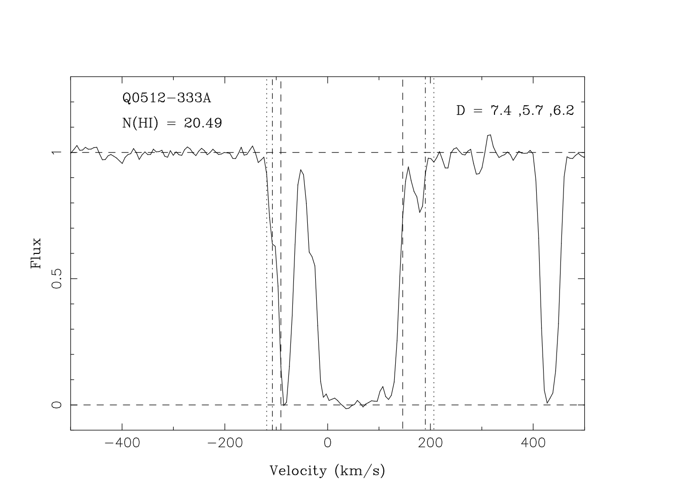
The values of EW and that are input into Eqn 1 are governed by the choice of . We have investigated the following possibilities: (i) defined by 3 absorption (described above and in Ellison 2006); (ii) defined by the central 90% of the Mg ii line EW. This is analogous to the technique used on unsaturated lines to determine the velocity width of an absorber based on optical depth (e.g. Prochaska & Wolfe 1997; Ledoux et al. 2006); (iii) defined by the central 90% of the velocity spread of the Mg ii line. As a further experiment, we apply these three techniques using the full spread of all Mg ii components in our calculation of the -index, in addition to the original definition of Ellison (2006) which uses only the main absorption complex. The D-index calculated over the central absorption excludes outlying components once the continuum has been recovered, whereas ‘full’ refers to all absorption components in a given Mg ii system. In Figure 3 we show how these different approaches yield different values for in one of the absorbers in our sample. This Figure is reproduced for all of our absorber sample in the online material that accompanies this article. We also provide in the online material a table listing all of the EWs and errors for the 3 approaches described above for each absorber; Table 4 gives the first four lines of the online version as an example.
| QSO | log N(HI) | EW90%EW(Å) | (km s-1) | EW90%vel(Å) | (km s-1) | EW3σ (Å) | (km s-1) |
|---|---|---|---|---|---|---|---|
| Q0823223 | 19.040.04 | 0.850.03 | 186.38 | 0.930.04 | 231.30 | 0.930.04 | 206.59 |
| Q1206459 | 19.040.04 | 0.560.02 | 106.86 | 0.630.03 | 142.48 | 0.630.03 | 115.76 |
| Q0424131 | 19.040.04 | 0.250.01 | 37.53 | 0.280.02 | 65.04 | 0.260.02 | 40.03 |
| Q0002051 | 19.080.04 | 0.620.03 | 95.03 | 0.660.04 | 129.80 | 0.630.02 | 85.76 |
In Table 5 we give the success statistics and optimal value for each technique33 3 The D-index statistics which include N(Fe ii) are described later in this section.. The success rate is defined as the fraction of systems with that are actually DLAs. The DLA miss rate is the fraction of DLAs with . We also tabulate the Kolmogorov-Smirnov (KS) probability that the -indices of sub-DLAs and DLAs for a given technique are drawn from the same population. Table 5 shows that all of the techniques yield more or less consistent results, with success rates 50 – 55 % and KS probabilities on the order of a few percent. As an example, we show the distribution of versus (H i) in Figure 4 when the 90% EW limits are applied to the central absorption complex.

| Absorption range | limits | Optimal | DLA success rate (%) | DLA miss rate (%) | KS probability (%) |
|---|---|---|---|---|---|
| Central | 3 | 6.7 | 48.6 | 19.0 | 9.1 |
| Central | 90% velocity | 5.5 | 54.3 | 9.5 | 0.1 |
| Central | 90% EW | 7.2 | 54.1 | 4.8 | 0.4 |
| Full | 3 | 6.3 | 51.5 | 19.0 | 5.3 |
| Full | 90% velocity | 5.2 | 53.1 | 19.0 | 2.4 |
| Full | 90% EW | 7.0 | 56.7 | 19.0 | 1.3 |
| Central + N(Fe ii) | 3 | 6.3 | 48.4 | 11.8 | 20.6 |
| Central + N(Fe ii) | 90% velocity | 5.7 | 57.7 | 11.8 | 0.1 |
| Central + N(Fe ii) | 90% EW | 7.0 | 57.1 | 5.9 | 0.5 |
| Full + N(Fe ii) | 3 | 5.2 | 55.6 | 16.7 | 1.3 |
| Full + N(Fe ii) | 90% velocity | 5.1 | 60.0 | 16.7 | 0.6 |
| Full + N(Fe ii) | 90% EW | 5.6 | 53.6 | 16.7 | 1.3 |
We next consider whether including information from other metal lines may improve the use of to distinguish DLAs and sub-DLAs. It has been shown (e.g. Meiring et al. 2008; Peroux et al. 2008) that sub-DLAs have a tendency to be more metal-rich than DLAs. Indeed, there is a lack of high (H i) high metallicity systems that empirically manifests itself as an apparent anti-correlation between (H i) and [Zn/H] (Boisse et al. 1998; Prantzos & Boissier 2000). Although it has been argued that this is due to dust bias, this interpretation is not supported by extinction measurements of DLAs (Ellison, Hall & Lira 2005). Simply put, the observed reddening values derived from DLA samples (Murphy & Liske 2004; Ellison et al. 2005; Vladilo, Prochaska & Wolfe 2008) are much lower than would be required to impose a ‘dust filter’. Moreover, it has been argued (Dessauges-Zavadsky et al. 2003) that the higher metallicities in sub-DLAs are not a result of ionization corrections. As we have shown above, any systematic error in the (H i) of low redshift sub-DLAs determined from low resolution spectra is both small, and in the wrong sense to explain the different metallicity distributions. In the absence of any experimental reason (such as dust bias or ionization correction) behind the elevated metallicities in sub-DLAs, we explore whether information on the metallicity of an absorber can be combined with the kinematic description encapsulated in Eqn 1 to improve the selection success of the -index.

In Figure 5 we show the distribution of [Fe/H] versus -index (as defined by the 90% EW range for the central absorption component) for the 49 absorbers for which N(Fe ii) measurements are available in the literature. It can be seen that in the regime of high -index, the DLAs have preferentially lower metallicities than the sub-DLAs. For , the mean [Fe/H] is for sub-DLAs and for DLAs. These mean values are calculated by treating the lower limits of the three absorbers with fully saturated Fe ii profiles as detections. The difference between the mean metallicities could therefore be even larger. Although the DLAs in our sample have a higher mean redshift than the sub-DLAs (see next section) the evolution of DLA metallicity is very mild. Kulkarni et al. (2005) show that the DLA metallicity changes by less than 0.3 dex from to . Of course, we can not use the actual metallicity to fine-tune the definition of the -index, since this requires a measurement of (H i), the very quantity we are hoping to select for. We therefore consider the use of N(Fe ii). In Figure 6 we show histograms of log N(Fe ii) for the compilation of DLAs and sub-DLAs in Dessauges-Zavadsky et al. (in prep.) at (the redshift regime for which we are trying to develop a selection technique). The column density of Fe ii is a quantity that can be measured with relative ease from almost any high resolution spectrum suitable for -index determination. There are almost a dozen different Fe ii transitions with a large dynamic range in -value at wavelengths not far from Mg ii. From Figure 6 we can see that the DLAs clearly have systematically higher N(Fe ii) than the sub-DLAs. The mean log N(Fe ii) (and standard deviation) is 15.150.08 for DLAs and 14.640.07 for sub-DLAs. Although the element zinc is usually considered the best indicator of actual metallicity, we emphasize here that we are simply using iron from the empirically motivated viewpoint that its column density is systematically different in DLAs and sub-DLAs.
We factor N(Fe ii) into our calculation of the -index by multiplying the value derived from Eqn 1 by log N(Fe ii) and dividing by 15 (to re-scale the D-index):
| (2) |
In Table 5 we give the success and miss rates for this modified -index definition, again calculating its value for the six different combinations investigated above and excluding systems which only have N(Fe ii) limits. Figure 7 shows the distribution of -index versus (H i) for our sample using the definition of D given in Eqn 2. Although the success rates generally improve slightly (by a few percent) when N(Fe ii) is included, this is not a significant improvement given the modest-sized sample. The close consistency of success rates with/without N(Fe ii) included in the calculation is probably due to the small relative difference (in the log) between iron column densities. It is also worth noting that in Figure 5 there is apparently no correlation between -index and [Fe/H] in DLAs, indicating that the -index does not preferentially select high or low metallicity DLAs. On the other hand, 4/5 sub-DLAs with have [Fe/H] , the highest values in our sample. Therefore, using low values of to select sub-DLAs may miss the highest metallicity absorbers.


4 Summary and discusssion
We have presented a sample of 56 Mg ii absorbers with known (H i) column densities and investigated techniques to screen for DLAs. The -index combines measures of both Mg ii EW and velocity spread, and we have also investigated incorporating information on the Fe ii column density. The results are robust to the various parameterizations that we use, with a typical DLA yield of 55%, compared to 35% when Mg ii EW alone is used (Rao et al. 2006). The relative insensitivity to the precise definition of the -index is reassuring, in the sense that it demonstrates that its success is unlikely to be a fluke of our dataset or choice of parameterization.
4.1 Using the -index
Given the results in Table 5, what is the ‘best’ definition of ? Given the sample size (and hence, rounding errors in the success and miss rates), simply selecting the technique with the best statistics is not necessarily the best choice. Instead, we consider which technique might be the most robust against issues such as noise, resolution and absorber environment. Any of the methods that use the ‘full’ velocity range will be sensitive to outlying components that may have nothing to do with the main absorber, e.g. be associated with a satellite galaxy. As discussed in Section 3.1, sub-DLAs in particular are known to often have companion absorbers. S/N is a consideration for techniques that use a 3 cut-off, either over the full absorption range, or just the central complex. However, Ellison (2006) showed that S/N only significantly degrades the efficiency of -index selection in the central absorption component at S/N . The disadvantage of using the 90% velocity range is that it is sensitive to small differences (between spectra) of resolution. As Ellison (2006) showed, this is also the case for a 3 definition. Taking these issues into account, and then re-visiting the statistics of Table 5, we suggest that the 90% EW over the central absorption range (i.e excluding outlying, low EW clouds), should be the most robust to these various troubles and yields a high success rate, with only one DLA missed. The optimal values of are very similar for the central/90% EW technique whether or not N(Fe ii) is included – 7.0 and 7.2 respectively. The KS test probability is slightly better when Fe ii is included.
One potential bias in the evaluation of the -index in the current sample is that the redshift distributions of the DLAs and sub-DLAs are not the same. The mean DLA redshift is , compared with 1.06 for the sub-DLAs, with very few of the latter above . This potential bias can be seen in Figures 4 and 7 where the open points show absorbers at . Confining our analysis to absorbers only in this low redshift range includes only 5 DLAs with Fe ii detections, insufficient for robust statistical analysis. However, Mshar et al. (2007) have shown that neither the EW distribution, nor the velocity spread of strong Mg ii systems evolves with redshift. These authors do, however, find differences in the number and distribution of ‘subsystems’ between their low and high redshift sample. Whilst the low redshift absorbers tend to comprise a single strong absorption component with one satellite subsystem, there are more subsystems in high redshift absorbers, over the same velocity range. The -index is sensitive to such differences. However, the redshift differences in kinematic structure reported by Mshar et al. (2007) and described above can not explain the ‘success’ of the -index in distinguishing DLAs from sub-DLAs. This is because the redshift inequality in our sample is such that we have more DLAs at high , where the tendency towards more complex kinematic structure would decrease the -index. However, DLAs are defined by high values of , i.e. with few kinematically extended subsystems. Further evidence against a redshift bias in our sample comes from Ledoux et al. (2006) who find that, in DLAs, the median velocity width of unsaturated metal lines increases with decreasing redshift. This redshift dependence again works in the opposite sense to a redshift bias that would artificially introduce a -index dependence in our work. Therefore, although it is certainly desirable to repeat the -index tests for a sample of sub-DLAs and DLAs that are matched in redshift, there is no empirical evidence to suggest that redshift evolution can explain the difference in .
In summary, we recommend that the -index is calculated using the 90% EW range over the central absorption complex, incorporating N(Fe ii), if available, see Equation 2. In Figure 7 we show the distribution of (H i) versus -index for this choice of parameters. This Figure is directly comparable to Figure 4 which uses the same definition of the -index, but does not include N(Fe ii) in the calculation. Based on our recommended definition, the KS probability that the -indices of sub-DLAs and DLAs are drawn from the same population is 0.5%. In our sample of 45 absorbers with accurate Fe ii column densities, 57% (16/28) of systems with 7.0, are DLAs where the error bars are 1 values taken from Gehrels (1986). Only 6% (1/17) of the DLAs in the sample of 45 have .
4.2 Interpretation of the -index
Ellison (2006) suggested that the -index may be driven in part by the QSO-galaxy impact parameter. For a galaxy composed of numerous Mg ii ‘clouds’, whose size is of the order of a few kpc (Ellison et al. 2004b), the absorption may appear more patchy when the sightline intersects at large impact parameter where the filling factor of these clouds is low. A sightline passing close to the galaxy’s centre will intercept a higher density of absorbing clouds, perhaps with a smaller radial velocity distribution. This picture is supported by empirical evidence that the EW of Mg ii absorbers does correlate with impact parameter (Churchill et al. 2000; Chen & Tinker 2008) and sub-DLAs do have more distinct absorbing components than DLAs (Churchill et al. 2000).
Another possible source of distinction between the kinematic structure of DLAs and sub-DLAs is the presence of galactic outflows. The connection between outflows and a subset of strong Mg ii absorbers has been discussed in the literature for several years (e.g. Bond et al. 2001; Ellison, Mallen-Ornelas & Sawicki 2003), although it remains contentious as a general description (see discussions in Bouché et al. 2006 and Chen & Tinker 2008). Nonetheless, galactic outflows are apparently common in high redshift star-forming galaxies (e.g. Shapley et al 2003; Weiner et al. 2008) and a growing body of empirical evidence is being published which supports the connection of strong Mg ii absorbers with winds or outflows. For example, Zibetti et al. (2007) find that the mean impact parameter of Mg ii absorbers in the SDSS is about 50 kpc from a L⋆ galaxy. One explanation for this observation is that the absorption detected in QSO spectra corresponds to material that is in a large extended region, possibly associated with winds. Ménard & Chelouche (2008) also argue for the connection of Mg ii absorbers to massive galaxies based on their gas-to-dust ratios, which are an order of magnitude higher than values for DLAs (Murphy & Liske 2004; Ellison et al. 2005; Vladilo et al. 2006). Murphy et al. (2007) observed a significant correlation between Mg ii EW and metallicity and concluded that ‘[there is] a strong link between absorber metallicity and the mechanism for producing and dispersing the velocity components’. Finally, Kacprzak et al. (2007) have shown that there is a correlation between the Mg ii EW and the degree of asymetry in the host galaxy. However, it does not necessarily flow that all strong Mg ii absorbers are connected with outflows. Both Bouché (2008) and Ménard & Chelouche (2008) have recently suggested that, when plotted in the (H i)-Mg ii EW plane, there are two separate absorber populations distinguished by metallicity. This effect is also seen in Figure 5 where the high -index absorbers are fairly cleanly separated into high metallicity sub-DLAs and low metallicity DLAs. Bouché (2008) proposes that the more metal-rich, lower (H i) absorbers at a given Mg ii EW are associated with galactic outflows. In turn, this may lead to kinematics that are more patchy in velocity space (e.g. Ellison et al. 2003) and contribute to the mechanism behind the success of the -index.
4.3 Applications of the -index
The -index requires moderately high resolution spectra to yield accurate pre-selection. Therefore, whilst EW-only DLA pre-selection can exploit the truly enormous datasets of, for example, the SDSS (e.g. Rao & Turnshek 2000; Rao et al. 2006), what is the niche for the -index? Individual groups have already used moderately large datasets for Mg ii searches at high resolution. The two most recent surveys for strong Mg ii absorbers in high resolution spectra are Mshar et al. (2007) (56 absorbers with 2796 EW 0.3 Å) and Prochter et al. (2006a) (21 absorbers with Mg ii 2796 EW 1 Å). Given that the number density of Mg ii 2796 EW 0.6 Å absorbers is a factor 2 larger than at 1 Å, these two samples would already yield over 50 absorbers suitable for -index screening (not accounting for an overlap between the samples). However, these samples are small compared to the full archival power that could be applied. After a decade of high resolution spectroscopy with HIRES on Keck and UVES at the VLT, and a somewhat shorter, but extremely productive history with ESI, we estimate that 500 – 700 QSOs have been observed at moderate–high resolution (e.g. Prochaska et al. 2007b). If we assume an average emission redshift =2.5 for 500 QSOs, and maximum wavelength coverage of 8500 Å, this yields a redshift path of almost 760. The number density of strong Mg ii absorbers has been robustly determined from SDSS spectra (e.g. Nestor et al. 2005; Prochter et al. 2006a). For example, Nestor et al. (2005) find that the number density of Mg ii 2796 EW 0.6 Å absorbers (a typical EW suitable for DLA pre-selection) at is . This value is unlikely to be affected due to magnitude bias (Ellison et al. 2004a) and can therefore also be applied to high resolution spectra. The total number44 4 We note that the sample used for the study in this paper does not have much overlap with this archival path length. of such absorbers that we could therefore expect to find in existing moderate–high resolution spectra is therefore approaching 400. Even though follow-up observations with space telescopes are likely to focus on the brightest in this sample, the typical magnitude limit for echelle spectroscopy with an 8-m ground-based telescope is close to the limit that will be feasible for the Cosmic Origins Spectrograph (COS) and the renovated STIS .
The -index may also be useful for assessing the nature of absorption where follow-up observations of Ly are not even possible. For example, in the spectra of GRBs. As observatories (and observers) fine-tune their rapid follow-up techniques, there is a growing database of bright GRBs that have been observed promptly at high resolution (e.g. Vreeswijk et al. 2007; Ellison et al. 2007; Prochaska et al. 2007a). Mg ii absorbers detected in these spectra that do not have Ly covered, have no chance of susbsequent follow-up due to the rapid fading of the optical afterglow, but their likelihood of being DLAs can still be assessed, (e.g. Ellison et al. 2006; Prochaska et al. 2007a). The application to GRB spectra is particularly interesting given the possibility of deep searches for the absorbing galaxy after the optical afterglow has faded. Even at low redshifts, the study of DLA host galaxies has been challenging with QSO impact parameters of 1–2 arcseconds (e.g. Chen & Lanzetta 2003 and references therein). Identifying probable DLAs in GRB spectra opens the door to host galaxy searches to unprecedented depths.
Finally, in light of the recent puzzling result by Prochter et al. (2006b) that intervening Mg ii absorbers are more numerous towards GRB sightlines than QSO sightlines, it would also be interesting to compare the distribution of -indices of these two populations.
Acknowledgments
SLE was funded by an NSERC Discovery grant. MTM thanks the Australian Research Council for a QEII Research Fellowship (DP0877998). We are indebted to Chris Churchill and Joseph Meiring for providing spectra that expanded our archival sample. Joe Hennawi provided valuable help in obtaining and reducing the HIRES data. This research has made use of the NASA/IPAC Extragalactic Database (NED) which is operated by the Jet Propulsion Laboratory, California Institute of Technology, under contract with the National Aeronautics and Space Administration.
References
- Asplund et al. (2005) Asplund, M., Grevesse, N., Sauval, A. J., 2005 ASP Conference Series, 336, 25
- Boisse et al (1998) Boisse, P., Le Brun, V., Bergeron, J., Deharveng, J.-M., 1998, A&A, 333, 841
- Bond et al (2001) Bond, N., Churchill, C., Charlton, J., Vogt, S., 2001, ApJ, 562, 641
- Bouché et al. (2006) Bouché, N., Murphy, M. T., Peroux, C., Csabai, I., Wild, V., 2006, MNRAS, 371, 495
- Bouché (2008) Bouché, N., 2008, arXiv:0803.3944v2
- Chen & Lanzetta (2003) Chen, H.-W., Lanzetta, K., 2003, ApJ, 597, 706
- Chen & Tinker (2008) Chen, H.-W., Tinker, J. L., 2008, ApJ, submitted, arXiv:0801.2169
- Churchill et al (1999) Churchill, C. W., Rigby, J R., Charlton, J. C., Vogt, S. S., 1999, ApJS, 120, 51
- Churchill et al (2003a) Churchill, C. W., Mellon, R. R., Charlton, J. C., Vogt, S., 2003a, ApJ, 593, 203
- Churchill et al (2003b) Churchill, C. W., Vogt, S., Charlton, J. C., 2003b, AJ, 125, 98
- Dessauges-Zavadsky et al. (2003) Dessauges-Zavadsky, M., Péroux, C., Kim, T.-S., D’Odorico, S., McMahon, R. G., 2003, MNRAS, 345, 447
- Dessauges-Zavadsky et al (2004) Dessauges-Zavadsky, M., Calura, F., Prochaska, J. X., D’Odorico, S., Matteucci, F., 2004, A&A, 416, 79
- Dessauges-Zavadsky et al. (2006) Dessauges-Zavadsky, M., Prochaska, J. X., D’Odorico, S., Calura, F., Matteucci, F., 2006, A&A, 445, 93
- Ellison & Lopez (2001) Ellison, S. L., & Lopez, S., 2001, A&A, 380, 117
- Ellison, Mallen-Ornelas & Sawicki (2003) Ellison, S. L., Mallen-Ornelas, G., & Sawicki, M., 2003, ApJ,589, 709
- Ellison et al. (2004) Ellison, S. L., Churchill, C. W., Rix, S. A., Pettini, M., 2004a, ApJ, 615, 118
- Ellison et al. (2004) Ellison, S. L., Ibata, R., Pettini, M., Lewis, G. F., Aracil, B., Petitjean, P., Srianand, R., 2004b, A&A, 414, 79
- Ellison, Hall & Lira (2005) Ellison, S. L., Hall, P. B., Lira, P., 2005, AJ, 130, 1345
- Ellison (2006) Ellison, S. L., 2006, MNRAS, 368, 335
- Ellison et al. (2006) llison, S. L., et al. 2006, MNRAS, 372, L38
- Ellison et al. (2007) Ellison, S. L., Hennawi, J. F., Martin, C. L., Sommer-Larsen, J., 2007, MNRAS, 378, 801
- Gehrels, N. (1986) Gehrels, N., 1986, ApJ, 303, 336
- Kacprzak et al. (2007) Kacprzak, G. G., Churchill, W. C., Steidel, C. C., Murphy, M. T., Evans, J. L., 2007, ApJ, 662, 909
- Kim et al. (2002) Kim, T.-S., Carswell, R. F., Cristiani, S., D’Odorico, S., Giallongo, E., 2002, MNRAS, 335, 555
- Kulkarni et al. (2005) Kulkarni, V., Fall, S. M., Lauroesch, J. T., York, D. G., Welty, D. E., Khare, P., Truran, J., W., 2005, ApJ, 618, 68
- Ledoux, Bergeron & Petitjean (2002) Ledoux, C., Bergeron J., & Petitjean, P., 2002, A&A, 305, 802
- Ledoux et al. (2003) Ledoux, C., Petitjean, P., Srianand, R., 2003, MNRAS, 346, 209
- Ledoux et al. (2006) Ledoux, C., Petitjean, P., Fynbo, J. P. U., Moller, P., Srianand, R., 2006, A&A, 457, 71
- Lopez et al (1999) Lopez, S., Reimers, D., Rauch, M., Sargent, W., Smette, A., 1999, ApJ, 513, 598
- Lopez et al. (2005) Lopez, S., Reimers, D., Gregg, M. D., Wisotzki, L., Wucknitz, O., Guzman, A., 2005, ApJ, 626, 767
- Meiring et al. (2006) Meiring, J., Kulkarni, V. P., Khare, P., Bechtold, J., York, D. G., Cui, J., Lauroesch, J. T., Crotts, A. P. S.Nakamura, O., 2006, MNRAS, 370, 43
- Meiring et al. (2007) Meiring, J. D., Lauroesch, J. T., Kulkarni, V. P., Peroux, C., Khare, P., York, D. G., Crotts, A. P. S., 2007, MNRAS, 376, 557
- Meiring et al. (2008) Meiring, J. D., Kulkarni, V. P., Lauroesch, J. T., Peroux, C., Khare, P., York, D. G., Crotts, A. P. S., 2008, MNRAS, 384, 1015
- Ménard & Chelouche (2008) Ménard, B., & Chelouche, D., 2008, MNRAS, submitted, arXiv:0803.0745
- Murphy & Liske (2004) Murphy, M. T., & Liske, J., 2004, MNRAS, 345, L31
- Murphy et al. (2007) Murphy, M. T., Curran, S. J., Webb, J. K., Menager, H., Zych, B. J., 2007, MNRAS, 376, 673
- Nestor, Turnshek & Rao (2005) Nestor, D. B., Turnshek, D. A., Rao, S. M., 2005, ApJ, 628, 637
- Noterdaeme et al. (2008) Noterdaeme, P., Ledoux, C., Petitjean, P., Srianand, R., 2008, A&A, 481, 327
- Peroux et al. (2003a) Péroux, C., Dessauges-Zavadsky, M., D’Odorico, S., Kim, T.-S., McMahon, R., 2003a, MNRAS, 345, 480
- Peroux et al (2003b) Peroux, C., McMahon, R. G., Storrie-Lombardi, L. J., Irwin, M., Hook, I. M., 2003b, MNRAS, 346, 1103
- Peroux (2008) Peroux, C., Meiring, J. D., Kulkarni, V. P., Khare, P., Lauroesch, J. T., Vladilo, G., York, D. G., 2008, MNRAS, 386, 2209
- Pettini et al. (1999) Pettini, M., Ellison, S. L., Steidel, C. C., Bowen, D. V. 1999, ApJ, 510, 576
- Pettini et al. (2000) Pettini, M., Ellison, S. L., Steidel, C. C., Shapley, A. E., & Bowen, D. V. 2000, ApJ, 532, 65
- Pettini et al. (2002) Pettini, M., Ellison, S. L., Bergeron, J., Petitjean, P., 2002, A&A, 391, 21
- Prantzos and Boissier (2000) Prantzos, N., Boissier, S., 2000, MNRAS, 315, 82
- Prochaska and Wolfe (1997) Prochaska, J. X., & Wolfe, A. M. 1997, ApJ, 487, 73
- Prochaska et al. (2001) Prochaska, J. X., Wolfe, A., Tytler, D., Burles, S., Cooke, J., Gawiser, E., Kirkman, E., O’Meara, J., Storrie-Lombardi, L., 2001, ApJS, 137, 21.
- Prochaska, Herbert-Fort & Wolfe (2005) Prochaska, J. X., Herbert-Fort, S., & Wolfe, A. M., 2005, ApJ, 635, 123
- Prochaska et al. (2007a) Prochaska et al., 2007a, ApJS, 168, 231
- Prochaska et al. (2007b) Prochaska, J. X., Wolfe, A. M., Howk, J. C., Gawiser, E., Burles, S. M., Cooke, J., 2007b, ApJS, 171, 29
- Prochter et al. (2006) Prochter, G. E., Prochaska, J. X., Burles, S. M., 2006a, ApJ, 639, 766
- Prochter et al. (2006) Prochter, G. E., Prochaska, J. X., Chen, H.-W., Bloom, J. S., Dessauges-Zavadsky, M., Foley, R. J., Pettini, M., Dupree, A. K., Guhathakurta, P., ApJ, 2006b, 648, L93
- Rao and Turnshek (2000) Rao, S.M., & Turnshek, D.A. 2000, ApJS, 130, 1
- Rao, Turnshek & Nestor (2006) Rao, S.M., Turnshek, D.A., Nestor, D. B., 2006, ApJ, 636, 610
- Shapley et al (2003) Shapley, A., Steidel, C., Pettini, M., Adelberger, K., 2003, ApJ, 588, 65
- Turnshek & Rao (2002) Turnshek, D. A., Rao, S. M., 2002, ApJ, 572, L7
- Vladilo et al. (2008) Vladilo, G., Prochaska, J. X., Wolfe, A. M., 2008, A&A, 478, 701
- Vreeswijk et al (2007) Vreeswijk et al., 2007, A&A, 468, 83
- Weiner et al. (2008) Weiner, B. J., et al., 2008, ApJ, submitted, arXiv:0804.4686
- Zibetti et al. (2007) Zibetti, s., Ménard, B., Nestor, D. B., Quider, A. M., Rao, S. M., Turnshek, D. A., 2007, ApJ, 658, 161
- Zych et al. (2008) Zych, B. J., Murphy, M. T., Hewett, P. C., Prochaska, J. X., MNRAS, 2008, submitted.