Charged-Higgs effects in $B\rightarrow(D)\tau\nu$ decays

Supersymmetric extensions of the standard model (SM) – or more generally extensions that require the existence of at least one additional Higgs doublet – generate new flavour-changing interactions already at tree-level via the exchange of a charged Higgs boson. The coupling of $H^{+}$ to fermions grows with the fermion mass. It is thus natural to look at (semi)leptonic $B$ decays with a $\tau$ in the final state to try to uncover this type of effects. In a two-Higgs-doublet-model (2HDM) of type II, where up-type quarks get their mass from one of the two Higgs doublets and down-type quarks from the other one, $H^{+}$ effects are entirely parametrized by the $H^{+}$ mass, $M_{H}$, and the ratio of the two Higgs vacuum expectation values, $\tan\beta=v_{u}/v_{d}$. They can compete with the exchange of a $W^{+}$ boson for large values of $\tan\beta$ [1]. In the minimal supersymmetric extension of the SM (MSSM), the tree-level type-II structure is spoilt by radiative corrections involving supersymmetry-breaking terms. The effective scalar coupling $g_{S}$ then exhibits an additional dependence on sparticle mass parameters when $\tan\beta$ is large $(q=u,c)$ [2, 3]:

where $\varepsilon_{0,\tau}$ denote sparticle loop factors. The correction induced can be of order one. However, the access to the Higgs sector remains exceptionally clean. In Eq.(1), $g_{S}$ has been normalized such that it gives the fraction of effects in the $B\rightarrow\tau\nu$ amplitude, which is very sensitive to $H^{+}$ exchange: $\mathcal{B}(B\rightarrow\tau\nu)/\mathcal{B}(B\rightarrow\tau\nu)^{SM}=|1-g_{S}|^{2}$. The $B\rightarrow D\tau\nu$ channel is less sensitive (though better in this respect than other modes such as $B\to D^{*}\tau\nu$) but, as we will see, exhibits a number of features that make it, too, play an important part in the hunt for the charged Higgs boson.

The current capabilities of $\mathcal{B}(B\rightarrow D\tau\nu)$ and $\mathcal{B}(B\rightarrow\tau\nu)$ to constrain $H^{+}$ effects are compared in Fig.1 for $g_{S}\geq 0$ (as is typically the case in the MSSM or the 2HDM-II). The lower sensitivity of the $B\rightarrow D\tau\nu$ mode comes from the different momentum dependence of the Higgs contribution with respect to the longitudinal $W^{+}$ one¹¹ 1 Note that the latter, though helicity-suppressed, is still (slightly) larger than the transverse $W^{+}$ contribution for all $q^{2}$ values.: $(d\Gamma(B\to D\tau\nu)/dq^{2})^{W_{\parallel}^{+}+H^{+}}\propto|1-g_{S}(q^{2}/M_{B}^{2})/(1-m_{c}/m_{b})|^{2}$ with $q\equiv p_{B}-p_{D}$. On the other hand, the theory prediction for $\mathcal{B}(B\rightarrow\tau\nu)$ suffers from large parametric uncertainties from the CKM matrix element $V_{ub}$ and the $B$ decay constant $f_{B}$. In contrast, $V_{cb}$ is known with better than $2\%$ accuracy from inclusive $B\to X_{c}\ell\nu\ (\ell=e,\mu)$ decays, $|V_{cb}|=(41.6\pm 0.6)\times 10^{-3}$ [4], and the form factors $f_{+}(q^{2})$ and $f_{0}(q^{2})$ describing the $B\to D$ transition are very well under control, as we now discuss in more detail.

To this end, we introduce the following conformal transformation:

which maps the complex $q^{2}$ plane, cut along $q^{2}\geq(M_{B}+M_{D})^{2}$, onto the disk $|z|<1$. The form factors $f_{+}$ and $f_{0}$ are analytic in $z$ in this domain, up to a few subthreshold poles, and can thus be written as a power series in $z$ after these poles are factored out ($i=+,0$) [10]:

where the function $P_{i}$ gathers the pole singularities and an arbitrary analytic function $\phi_{i}$ can be factored out as well.

This parametrization has been used in Ref.[11] with the choice $t_{0}=q^{2}_{\textrm{max}}=(M_{B}-M_{D})^{2}$, together with heavy-quark spin symmetry inputs, to derive the following ansatz for the vector form factor:

where $V_{1}$ is defined such that it reduces to the Isgur-Wise function in the heavy-quark limit and $\mathcal{G}(1)\equiv V_{1}(q^{2}_{\textrm{max}})$. The parameters $|V_{cb}|\mathcal{G}(1)$ and $\rho^{2}$ can be determined from $B\to D\ell\nu$ experimental data. Before this summer, the HFAG averages [8] based on BELLE, CLEO, and ALEPH data read: $|V_{cb}|\mathcal{G}(1)=(42.3\pm 4.5)\times 10^{-3}$ and $\rho^{2}=1.17\pm 0.18$ (with a $|V_{cb}|\mathcal{G}(1)$-$\rho^{2}$ correlation of $0.93$). The recent BABAR results [12] and [13] have now been included, leading to a substantial improvement [5]: $|V_{cb}|\mathcal{G}(1)=(42.4\pm 0.7\pm 1.4)\times 10^{-3}$ and $\rho^{2}=1.19\pm 0.04\pm 0.04$ (with $|V_{cb}|\mathcal{G}(1)$-$\rho^{2}$ correlation $0.88$). The old and new vector form factors are compared in Fig.2 (left), where we have defined as usual $w=(M_{B}^{2}+M_{D}^{2}-q^{2})/(2M_{B}M_{D})$.

For the scalar form factor, we adopt the ansatz of Ref.[14]:

where $t_{0}=(M_{B}+M_{D})^{2}\left(1-\sqrt{1-(M_{B}-M_{D})^{2}/(M_{B}+M_{D})^{2}}\,\right)$ such that $|z|_{\textrm{max}}$ is minimized, $M_{1}=6.700\,\mbox{GeV}$ and $M_{2}=7.108\,\mbox{GeV}$ [15] are the subthreshold poles, and $\phi_{0}$ is obtained from Eq.(10) of Ref.[14] setting $Q^{2}=0$ and $\eta=2$:

Following [16], we truncate the series (3) after the first two terms. This is motivated by the fact that $|z|_{\textrm{max}}=0.032$ and that a similar parametrization for $f_{+}$, when fitted to experimental data, produces the same result as Eq.(4) in very good approximation [16]. Then, $|V_{cb}|a^{0}_{0}(t_{0})$ and $|V_{cb}|a^{0}_{1}(t_{0})$ are determined imposing the conditions (i) $|V_{cb}|S_{1}(0)=|V_{cb}|V_{1}(0)$ and (ii) $|V_{cb}|S_{1}(q^{2}_{\textrm{max}})=(4.24\pm 0.27)\%$ (corresponding to $|V_{cb}|=(41.6\pm 0.6)\times 10^{-3}$ from $B\to X_{c}\ell\nu$ [4] and $S_{1}(q^{2}_{\textrm{max}})=1.02\pm 0.05$ from HQET [16]). The scalar form factors obtained in this way from the old and new $|V_{cb}|V_{1}$ are not very different, as one can see on Fig.2 (right).

The recent progress on $|V_{cb}|V_{1}$ allows to reduce the errors on the SM predictions for the two $B\to D\tau\nu$ branching fractions: $\mathcal{B}(B^{-}\rightarrow D^{0}\tau^{-}\bar{\nu})^{SM}=\left(0.70^{+0.06}_{-0.05}\right)\%$, $\mathcal{B}(\bar{B}^{0}\rightarrow D^{+}\tau^{-}\bar{\nu})^{SM}=\left(0.65^{+0.06}_{-0.05}\right)\%$ (differing essentially due to $\tau_{B^{0}}\not=\tau_{B^{+}}$). The errors from $|V_{cb}|V_{1}$, however, already cancel to a large extent in the ratio $R\equiv\mathcal{B}(B\to D\tau\nu)/\mathcal{B}(B\to D\ell\nu)$, which is why the nice improvement in Fig.2 has little impact on Fig.1 (right), already dominated by the error on $S_{1}(q^{2}_{\textrm{max}})$: $R^{SM}=0.31\pm 0.02$. This estimation is compatible with the one obtained from lattice methods: $R^{SM}_{latt}=0.28\pm 0.02$ [17]. Note that replacing condition (ii) by a constraint on $S_{1}(q^{2}_{\textrm{max}})/V_{1}(q^{2}_{\textrm{max}})$ from HQET would lead to a similar error on $R$. Still, an interesting $95\%$ C.L. bound on $g_{S}$ can already be obtained from $R$: $g_{S}<1.79$, complementary to the bounds from $\mathcal{B}(B\rightarrow\tau\nu)$: $g_{S}<0.36\ \cup\ 1.64<g_{S}<2.73$. The corresponding exclusion zones in the $(M_{H},\tan\beta)$ plane are depicted in Fig.3. The error assigned to $S_{1}(q^{2}_{\textrm{max}})$ is quite conservative, so the above constraints are robust. At the three-sigma level, it is not possible to extract any interesting bound from $R$ yet, but its experimental knowledge is expected to improve in the near future. Its role to constrain $H^{+}$ effects will then of course depend on the new central value. For the moment, a $15\%$ measurement with the same central value would exclude $g_{S}>0.29$ at the $95\%$ C.L..

If a hint for a charged Higgs boson is seen at the branching fraction level, $B\to D\tau\nu$ has a great advantage over $B\to\tau\nu$: it allows to analyze the same data points on a differential basis, better suited to discriminate between effective scalar-type interactions and other effects. The $d\Gamma(B\to D\tau\nu)/dq^{2}$ distribution, in particular, has already been studied in great detail [18]. The polarization of the $\tau$ is also known as a $H^{+}$ analyzer [19], yet it requires the knowledge of the $\tau$ momentum, which cannot be accessed at $B$ factories as the $\tau$ does not travel far enough for a displaced vertex and decays into at least one more neutrino.

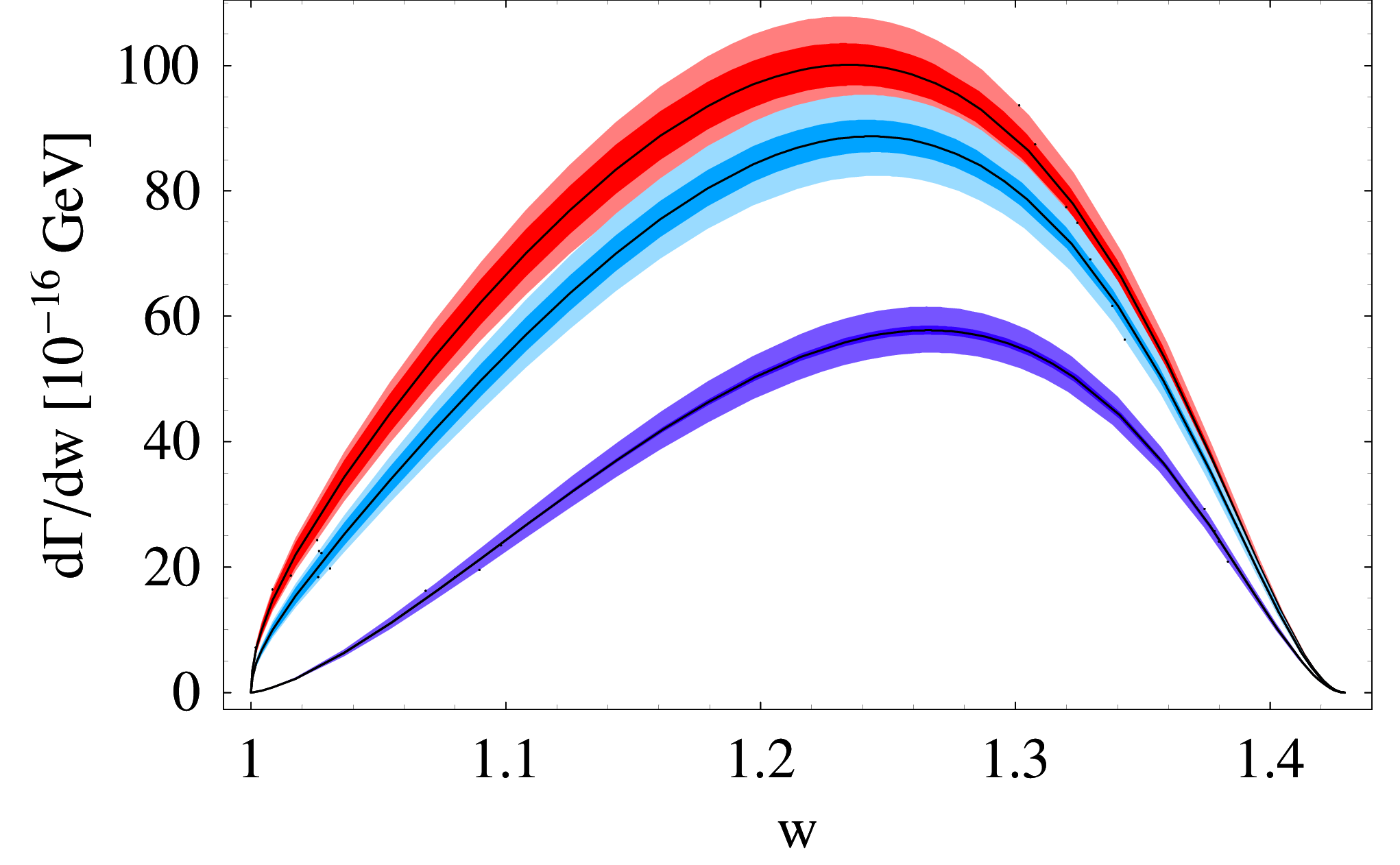
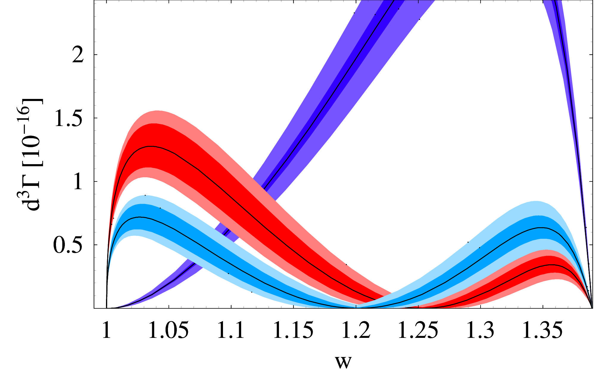
A straightforward way to nevertheless exploit the sensitivity of the $\tau$ polarization to $H^{+}$ effects and at the same time retain the information from the $q^{2}$ spectrum is to look at the subsequent decay of the $\tau$ into a pion and a neutrino [16]. The direction of the pion is indeed directly correlated with the polarization of the $\tau$. Integrating over the neutrino momenta, we end up with a triple differential decay distribution $d\Gamma(B\to D\nu\tau[\to\pi\nu])/dq^{2}dE_{\pi}d\cos\theta_{D\pi}$. An explicit formula is given in Eqs.(9-11) of Ref.[16] (with $F_{V}\equiv f_{+}$ and $F_{S}\equiv f_{0}$). Its sensitivity to $g_{S}$ is illustrated in Fig.4 for $E_{\pi}=1.8\,\mbox{GeV}$ and $\cos\theta_{D\pi}=-1$. For comparison, we also display the $q^{2}$ spectra corresponding to the same $g_{S}$ values. Of course, in practice, one should not fix $E_{\pi}$ or $\theta_{D\pi}$, but rather perform a (unbinned) maximum likelihood fit of the triple differential decay distribution to the available data points. The information from the $q^{2}$ spectrum in the dominant $\tau\to\ell\nu\bar{\nu}$ decay channel should also be included in the fit to make the most out of experimental data.

The form factors $f_{+}(q^{2})$ and $f_{0}(q^{2})$ in the $B\rightarrow D\tau\nu$ transition are under good control. As a result, the ratio $R\equiv\mathcal{B}(B\to D\tau\nu)/\mathcal{B}(B\to D\ell\nu)$ can be predicted with $7\%$ accuracy in the SM: $R^{SM}=0.31\pm 0.02$, where the $5\%$ uncertainty on the scalar form factor at zero recoil $S_{1}(q^{2}_{\textrm{max}})$ is the main error source. This allows to derive useful constraints on the effective $H^{+}$ coupling $g_{S}$. Together with the constraints from $\mathcal{B}(B\rightarrow\tau\nu)$, we obtain: $g_{S}<0.36\ \cup\ 1.64<g_{S}<1.79$, i.e., the window around $g_{S}=2$ left over by $\mathcal{B}(B\rightarrow\tau\nu)$ is now nearly completely excluded by $R$ alone. These bounds should be strengthened soon thanks to the current considerable experimental efforts on both modes. In this respect, one should pay particular attention to the $B\rightarrow D\tau\nu$ differential distributions as these are especially well-suited to discriminate between effective scalar interactions and other types of effects and, if the former are seen, to extract the coupling $g_{S}$ with good precision.