PITHA 08/26
SFB/CPP-08-81
October 18, 2008
decays revisited
M. Benekea,b and L. Vernazzaa
a Institut für Theoretische Physik E,
RWTH Aachen University,
D–52056 Aachen, Germany
b Institut für Theoretische Physik,
Universität Zürich,
CH – 8057 Zürich, Switzerland
We demonstrate that exclusive decays to -wave charmonium factorize in the non-relativistic limit provided that colour-octet contributions are taken into account, and estimate the branching fractions. Although there are very large uncertainties, we find reasonable parameter choices, where the main features of the data – large corrections to (naive) factorization and suppression of the and final states – are reproduced though the suppression of is not as strong as seen in the data. Our results also provide an example, where an endpoint divergence in hard spectator-scattering factorizes and is absorbed into colour-octet operator matrix elements.
1 Introduction
Exclusive two-body meson decays factorize in the heavy quark limit when the final state meson , that does not pick up the spectator antiquark from the meson, is light [1, 2, 3]. The reason for this is that the quark-antiquark progenitor of the “emitted” meson escapes the decay region as an object of small transverse size, which remains invisible to soft-gluon interactions with the transition [4]. This argument extends to any colour-singlet object that is small compared to the inverse strong interaction scale, . In particular, it has been suggested [2] that exclusive decays to charmonia , such as , should factorize in the heavy-quark and non-relativistic limit, when the charmonium radius . This expectation has been confirmed for decays to the -wave charmonia and by explicit next-to-leading order (NLO) calculations [5, 6, 7].11 1 Some of these papers use a light-cone rather than non-relativistic description of the charmonium, but this does not affect the conclusion. However, when the formalism was applied to -wave charmonium states [8, 9, 10, 11, 12, 13] infrared (IR) divergences appeared that seem to violate factorization.
In this paper we revisit this problem and show that factorization is recovered, if one includes the charmonium bound-state scales , (with a characteristic velocity of the charm quark in the bound state, ) into the theoretical framework. These scales are assumed to be intermediate between the heavy quark masses , and the strong interaction scale . The divergence structure described above bears resemblance with inclusive charmonium decay or production in the colour-singlet model. As is well-known the IR divergence problem in the -wave colour-singlet amplitudes is resolved by the introduction of colour-octet operators [14]. We shall see below that a similar mechanism is at work for . However, there is an important difference between -wave charmonium production in inclusive decay [15, 16] and exclusive decays. While in the former the charmonium decouples from the inclusive transition below the heavy quark mass scale, or at least is assumed to in previous treatments, this decoupling takes place for exclusive decays only below the scale of the binding energy , since gluons with this energy can reconnect to the system. In the (formal) heavy-quark limit this effect is perturbatively calculable since , and we shall provide numerical estimates for this contribution, which has been neglected in previous calculations. In the real world, , and hence reliable calculations appear to be hard to come by for decays to charmonium, contrary to decays to light .
In Table 1 we collect the current branching fraction measurements for the decays in question [17, 18, 19, 20, 21, 22, 23, 24, 25, 26, 27, 28, 29, 30, 31, 32, 33], including the -wave final states. By comparing to the -waves, we conclude that the -wave suppression is almost absent. Recalling that in naive factorization only the state is produced, the pattern of the -wave results is even more striking, and suggests significant decay amplitudes beyond naive factorization. The colour-octet contributions that we identify here may well be the dominant decay amplitudes, although they turn out to be hard to calculate for real-world charmonium. Nevertheless, it is interesting to see whether something can be said from theory that may help to understand the pattern of experimental data.
| — |
The infrared divergence in hard spectator-scattering is actually an endpoint divergence in a momentum-fraction convolution integral. Such endpoint divergences prohibit hard-scattering factorization of power-suppressed effects in non-leptonic decays to light mesons [1], and of to light meson form factors even at leading power [35, 36]. Understanding whether and how such endpoint divergences can be factorized remains a major challenge to theory. In decays to -wave charmonia the endpoint singularity also arises at leading order in the expansion, but we shall show that it can be factorized into the matrix elements of colour-octet operators. This is of some conceptual interest, since it is not known in general how to factorize endpoint divergences.
Two recent papers [37, 38] also discuss factorization of decays to charmonium. These papers deal with the leading order in the non-relativistic velocity expansion applicable to decays to -wave charmonia, but do not address -waves. The term “factorization” there refers to the heavy-quark mass scale or , and should thus be distinguished from its use here. While it is evident that decays to -wave charmonia do not factorize at the heavy-quark mass scale due to the infrared divergences mentioned above, our concern is to show that perturbative factorization is recovered when as conjectured in [2]. Corrections to naive factorization for decays to charmonium have also been estimated with light-cone QCD sum rules [39, 40, 41], but with this method the issue of infrared singularities in the QCD factorization result is not addressed.
2 Operator definitions and tree-level results
2.1 Effective Hamiltonian and kinematics
The effective weak–interaction Hamiltonian for the transition is
| (1) |
with
| (2) |
and neglecting the small contributions from the penguin operators.
The following notation is adopted for the kinematics of the two-body decay process : is the momentum of the meson, with ; of the charmonium, with the charmonium 4-velocity ( being the charmonium mass) with ; defines the relative momentum of the quark inside the charmonium, so that , with ; is the momentum of the kaon. Since kaon mass effects can be neglected in the heavy quark limit, the vector ( being the kaon energy in the rest frame) is light-like. The opposite-pointing light-like vector is denoted with . We also define , equal to up to corrections of order22 2 Note the dual use of : in power-counting estimates denotes the small relative velocity of the heavy quarks in the charmonium in the rest frame of the charmonium. In kinematical relations is the charmonium velocity vector. and . From energy-momentum conservation
| (3) |
For any vector (or Lorentz index ) the components transverse to and are denoted by (), for those orthogonal to we use (). Thus
| (4) |
2.2 SCET/NRQCD operator definitions
The bottom and charm quark masses are assumed to be heavy, with fixed in the heavy-quark limit. Integrating out the heavy quark mass scales , leads to an effective theory, in which the quark is static as in heavy-quark effective theory, the charm quarks are non-relativistic (in their center-of-mass frame) as in NRQCD and the light quarks are collinear (or soft) as in soft-collinear effective theory (SCET). The situation is similar to the corresponding one for charmless decays [42, 43, 44], except that the meson that does not absorb the spectator quark is now described by non-relativistic rather than collinear fields.
To build the decay operators in the effective theory below the heavy quark scale, we introduce the non-relativistic bilinears
| (5) |
of non-relativistic quark () and anti-quark () spinor fields.33 3 denotes the symmetric, traceless part of the tensor . It is convenient to use a covariant generalization of the NRQCD Lagrangian, where the non-relativistic fields are four-component spinors satisfying and . In the charmonium rest frame the non-zero spinor components reduce to the familiar non-relativistic two-spinors, and the components of a contravariant index equal the spatial components.
Then, adopting the SCET notation defined in [44], we construct the colour-singlet operators
| (6) | |||||
| (7) |
associated with the vertex and spectator-scattering amplitudes that have been considered in previous works [8, 9, 10, 11, 12, 13]. The operators are written in such a way that their tree-level matrix elements are proportional to the form factor times the derivative of the quarkonium wave function at the origin, since the expression in square brackets in (6) is the SCET representation of the full QCD form factor [45]. The effective vertices generated by the - and -type operators (in light-cone gauge, where ) are shown in Figure 1. New and central to the present discussion are the colour-octet operators
| (8) |
According to the assumption that charmonium is a Coulomb bound state, there exist two sets of low-energy scales, related to the non-relativistic expansion and , , related to the collinear expansion and the strong-interaction scale. In the case of charmless decays the matrix elements of colour-octet operators can be non-zero only due to power-suppressed soft-gluon interactions, where soft means momentum of order , thus they can be neglected at leading order in the expansion. For charmonium, however, the decoupling of gluons with small momentum holds only when the momentum is much smaller than ; gluons with momentum contribute to the octet operator matrix elements even at leading order in . These contributions are subleading in , but so are the -wave operators due to the extra derivative in , hence the gluon-exchange contribution to the -wave octet operators is relevant at leading order in the velocity expansion to -wave charmonium production.

Concentrating on the terms relevant to -wave production at leading (non-vanishing) order in the and expansion, the effective weak-interaction Hamiltonian below the heavy quark mass scale is therefore given by
| (9) | |||||
where we introduced the short-distance coefficients and .
2.3 Tree-level matching of -type operators
The leading-order matching coefficients are found by comparing the tree amplitude (topology as in the left diagram of Figure 1) computed with the effective Hamiltonian (1) to the corresponding amplitude from (9). The result is:
| (10) |
Since the matrix elements of the colour-octet operators and spectator-scattering are both suppressed by a factor of , this reproduces the well-known result from naive factorization that only the state is produced at leading order.
2.4 Estimate of the branching fraction
The leading-order decay amplitude is now given by the expression
| (11) |
The hadronic matrix element factorizes at leading order in the expansion in and according to
| (12) | |||||
where the two factors reduce to the QCD form factor,
| (13) |
and the derivative of the charmonium wave function at the origin:
| (14) |
with
| (15) |
Here spin symmetry of the leading non-relativistic interactions has been used to write all four matrix elements in terms of , or equivalently , where denotes the radial Schrödinger wave function of the , -wave states, and the prime denotes a derivative.
Squaring the amplitude, integrating over the two-body phase space, where we neglect the kaon mass, and summing over the charmonium polarizations with the help of
| (16) |
we obtain the branching fraction
| (17) | |||||
Due to (10) this is different from zero at leading order only for the state. With parameters as given in Section 5, varying the renormalization scale between 2 and 4.8 GeV, and between 1.45 and 1.75 GeV, we find
| (18) |
The largest uncertainty arises from the scale-dependence of the “colour-suppressed” Wilson coefficient . The naive factorization prediction is at least a factor of four smaller than the experimental result, see Table 1. This analysis shows that the dominant contribution to the decay amplitude comes, for -wave final state, from (naively) non-factorizable dynamics, such as radiative corrections, spectator-scattering, and the colour-octet contributions.
2.5 Overview of next-to-leading leading order terms
The leading contribution to (9) comes from the colour-singlet -wave A-type operators . Not including the fields themselves in the power-counting estimate, this contribution is of order , where the factor arises from the derivatives in the non-relativistic -wave operators (5) and the factor is from the tree-level coefficient function. Our intention is to show that radiative corrections can be consistently computed, when , so we now discuss the terms arising at order :
- 1.
One-loop corrections to the short-distance coefficients of the -wave colour-singlet operators (“vertex corrections”):
(19) where and equals the factorized matrix element (12).
Loop corrections to the matrix elements of these operators need not be considered. In particular, corrections to the factorization relation (12) are suppressed by powers of , or , where the two powers of the coupling arise from the vanishing colour-projection of one-gluon exchange.
- 2.
The tree-level matrix element of the B-type -wave colour-singlet operators is of order , since one factor of is in the definition of the operator and another is provided by the coupling of the collinear gluon to the spectator-quark line (“spectator-scattering”). The B-type form factor is of the same order as [46], hence this contribution is also of order . The hard spectator-scattering amplitude is
(20) - 3.
The colour-octet operators are of order , but their tree-level matrix elements vanish. The matrix element is non-zero due to soft gluon exchange between the charm-quark lines and the -quark and light-quark lines, including the spectator quark. At order , one must include the one-loop matrix element with exchange of a gluon of momentum :
(21) Loop corrections to the short-distance coefficients need not be considered, since the tree-level matrix element vanishes.
Colour-singlet -wave operators contribute only at higher orders due to the vanishing colour projection in the one-gluon exchange contribution to their matrix elements.
3 Short-distance contributions
3.1 One-loop short-distance coefficients

The one-loop correction to the short-distance coefficients of the A-type colour-singlet -wave operators (6) are obtained from matching the QCD diagrams in Figure 2 to the expression (19). There is no contribution from the diagram (not shown in the figure) with gluon exchange between the - and the -quark line, since the amplitude at tree-level involves only the form factor , which our operator definition reproduces exactly, but not .
The loop correction is expected to be large, since it comes with the large Wilson coefficient , while the tree amplitudes are either zero or colour-suppressed. We write
| (22) |
where the extra term in arises from the vertex correction in the second line of Figure 2. The loop functions are extracted from the amplitude expanded to first order in the relative momentum . The expansion is done in the integrand to extract the hard momentum region, and the integration is performed after expansion. The decomposition into the four angular momentum states is done according to the operators in (5). We use dimensional regularization with for both ultraviolet and infrared singularities, and the NDR scheme (naive anti-commuting ) for the treatment of and the definition of the weak effective Hamiltonian (1). Ultraviolet divergences are subtracted according to the prescription. An ultraviolet divergence is present only in , since for there exists a non-zero tree amplitude, while infrared divergences appear for the other -wave operators but not for . This can be understood from the fact that the infrared divergences are related to the and colour-octet matrix elements, and that soft gluons change angular momentum by one unit, but do not change spin.
Defining the auxiliary function
| (23) | |||||
and the ratio of heavy quark pole masses, we find
| (24) | |||||
The infrared pole, which violates factorization at the heavy quark mass scale, is exhibited explicitly in . One should note the difference with decays to light mesons or -wave charmonia, where the same hard vertex corrections are infrared finite. The singularity arises here as a consequence of the expansion to first order in the relative momentum , and signals that – unsurprisingly – the colour-transparency argument does not hold at the heavy-quark mass scale.
Results for the hard vertex correction, corresponding to the first four diagrams in figure 2, have been obtained previously in [8, 9, 10, 11, 12, 13], where the infrared divergences were noted for the first time. These papers use a gluon mass rather than space-time dimension as infrared regulator, while the finite part is given only in parametric form. This makes difficult to compare these result with ours, except for the infrared divergent part, where we agree, and for the case, where the finite contribution is given explicitly [12] and there is no infrared regulator dependence, and where we also agree. The fifth diagram in Figure 2 was not taken into account in previous papers.
3.2 Short-distance spectator scattering

The tree contribution to the short-distance coefficients of the -type colour-singlet -wave operators (7) is obtained from matching the QCD amplitude for the process shown in Figure 3 to the expression (20). In this way, we calculate directly the momentum-space coefficient function
| (25) |
where is the fraction of longitudinal momentum carried by the hard-collinear gluon. We find
| (26) |
For later purposes it will be useful to express these results as
| (27) |
with -independent coefficients , , which follow by comparison with (26).

The hard spectator-scattering amplitude (20) requires the evaluation of the convolution
| (28) |
which is done following [44]. The corresponding diagram is shown in Figure 4. First, as in the case of the A-type operators, the tree matrix element factorizes according to
| (29) | |||||
The heavy-to-light matrix element is the same as appears in non-leptonic decay to two light mesons resulting in ([44], Eqs. (6), (8))
| (30) |
Here and are the leading-twist light-cone distribution amplitudes of the and the meson, respectively, while the hard-collinear “jet function” is given at leading order by
| (31) |
Introducing
| (32) |
the tree-level matrix elements reads
| (33) |
Inserting the Fourier representation of the coefficient function into (28), we find the amplitude
| (34) | |||||
This result has been obtained previously [8, 9, 10, 11, 12] by direct evaluation of the spectator-scattering amplitude.
The problematic aspect of this expression is the endpoint divergence of the convolution integral when . The kaon light-cone distribution amplitude behaves as for small . But contrary to the situation for decays to two light mesons or an -wave charmonium and a kaon, the coefficient function contains a piece proportional to resulting in a logarithmically divergent integral. We regularize this integral by introducing a cutoff that replaces the upper limit by with . Using
| (35) |
the convolution integral in (34) takes the final form
| (36) |
The regulator-dependent term appears to violate factorization even at leading power in the heavy quark expansion. We shall show below, however, that this dependence is canceled by a corresponding ultraviolet divergence in the colour-octet matrix elements.
4 Colour-octet matrix elements
The important new element in our treatment of decays to -wave charmonia are the colour-octet contributions (9), (21) to the decay amplitude. We shall now show how to compute these matrix elements when the charmonium is a Coulomb bound state and demonstrate that the infrared singularities in the vertex correction and hard spectator-scattering can be absorbed into a renormalization of the colour-octet matrix elements. In the Coulomb limit the octet matrix elements can be computed in perturbation theory, and we provide results at order , corresponding to the accuracy of the short-distance terms. In general, and more realistically, the colour-octet matrix elements may be introduced as new non-perturbative parameters, but their scale dependence still cancels the factorization scale dependence of the hard-scattering terms. However, factorization in the sense of separating the transition from the vacuum to charmonium matrix element holds only in the Coulomb limit, since otherwise the octet matrix elements of the SCET/NRQCD four-quark operators contain strongly interacting gluon exchanges between the charmonium and the system.
4.1 Reduction formula for quarkonium matrix elements
We briefly review the formalism for the calculation of quarkonium matrix elements
| (37) |
where is some operator, the quarkonium with momentum in some polarization state, and , denote arbitrary other particles.

The quarkonium matrix element is identified in the standard way as part of the residue factor of the pole of a suitable Green function. We pick a Green function with two external charm quark fields. The quarkonium bound state poles appear after summing ladder diagrams with colour-singlet Coulomb (potential) gluon exchange as the bound state poles of the Coulomb Green function as indicated in Figure 5. For external momenta with near the bound state poles appear in the integration region where , with and , small, of order and , respectively. A specific charmonium state is extracted by performing the following steps: (1) Insert the spectral representation of the Green function and use that near a bound state pole
| (38) |
where is the momentum space wave function of the Schrödinger operator in the basis. The three-vectors are introduced by writing four-vectors orthogonal to as , where and is the Lorentz boost from the quarkonium rest frame to the frame where its momentum is . (2) To separate the degenerate states with different angular momentum and spin, first introduce the spherical decomposition
| (39) |
defining . Then perform a Fierz transformation in the Dirac indices of the two intermediate charm propagators in Figure 5 to obtain the projection on the spin zero and spin 1 components. For , the states follow from the standard Clebsch-Gordon relations.
The final result can be expressed in terms of the on-shell matrix element corresponding to (37), which we write in the from
| (40) |
Defining the matrices
| (41) |
in Dirac-index space (and diagonal in colour space), the desired quarkonium matrix element is
| (42) |
This is valid in a leading-order treatment of the non-relativistic bound state dynamics. Beyond this approximation, corrections to the wave-function and trace expression are required. Eq. (42) can be used to calculate the first non-vanishing contribution to a quarkonium matrix element, and this will be sufficient for the colour-octet terms considered below.
The momentum-space radial wave function follows from the Fourier transform of the position-space expression and is given by
| (43) |
For the case , , using the spherical Bessel function
| (44) |
the integral evaluates to
| (45) |
where denotes the derivative of the position-space wave function at the origin, and
| (46) |
is the inverse Bohr radius of the charmonium.
4.2 Soft vertex correction
We proceed to the calculation of the colour-octet matrix elements and (). Note that at order the interactions are spin-symmetric, so there is no contribution of the () operator to the () final state. Each matrix element receives contributions from vertex diagrams (first four diagrams in Figure 2) and spectator-scattering diagrams (Figure 3 with gluon attached to the undisplayed spectator quark line), except that now the gluon virtuality is small, of order for the vertex diagrams.
We begin by writing down the soft gluon coupling to the pair. The leading interactions of dynamical gluons with momentum of order to the heavy charm quarks are provided by the (P)NRQCD effective Lagrangian. They read together with a similar term for the antiquark field. The contribution from the coupling cancels in the sum of the attachments to the and the line (or can be gauged away), leaving the chromoelectric dipole interaction. The dipole interaction provides the additional factor of velocity which renders the octet -wave operator matrix element of the same order in as the singlet -wave operator.
The part of the amplitude involving the charm quark lines can now be expressed in the form
| (50) |
see Figure 6. The various items in this equation are as follows: denotes the outgoing soft gluon momentum; comes from the part of the colour-octet operator as given by the contents of square brackets in (5); is the momentum-space soft gluon interaction vertex
| (51) |
where and “B” are, respectively, the Lorentz and colour index of the soft gluon; is the Coulomb Green function that sums an infinite number of gluon exchanges “between” the operator and the soft gluon vertex. Here we need the colour-octet Green function, since the pair is produced at the operator vertex in a colour-octet state. The calculation of the vertex diagrams with the full Coulomb Green function is quite involved (see [47] for the calculation of colour-octet inclusive quarkonium production matrix elements), but turns out to be unnecessary to good approximation. Similar calculations involving colour-octet Coulomb Green functions [48, 49] find that the numerically largest term arises from the no-gluon exchange term, since every colour-octet exchange is suppressed by the small colour factor . We therefore simplify (50) by approximating
| (52) |
obtaining
| (53) |

Attaching the gluon to the bottom quark and the strange quark line and making use of (42), we arrive at
| (54) | |||||
where we used that is soft to simplify the bottom and strange quark propagators, and denote the binding energy by
| (55) |
The colour index “A” is contracted with an index hidden in the definition of , while and “B” are contracted with the corresponding indices in (53). The order of the colour matrices , which is different for the attachment to the bottom and strange line plays no role, since the colour part of the trace evaluates to . The corresponding matrix elements of the operators have instead of in the matrix element. The absence of a transverse vector implies that the matrix element vanishes, so at this order
| (56) |
The integrations appearing in (54) can be performed exactly. The loop integral is of the general form
| (57) |
Only enters the final result, and can be calculated directly by introducing Feynman parameters. In contrast to the hard vertex correction, this loop integral is infrared finite. The sensitivity to very soft gluon momenta is cut off at the scale of the binding energy since . On the other hand, there is a logarithmic ultraviolet divergence, which we regulate dimensionally to be consistent with the calculation of the short-distance correction. The angular -integral is also easily done using44 4 Note .
| (58) |
The remaining -integral is of the type
| (59) |
with -independent constants , , and is evaluated using the explicit form (45) of the momentum-space radial wave function. Including the colour and spin traces we find
| (60) |
where we have re-expressed the product of the derivative of the wave function at the origin and the form factor in terms of the factorized matrix element (12) to facilitate the comparison with the hard vertex amplitude (19). Eq. (60) contains the spin-dependent coefficients and (for ), and the loop function
| (61) |
This includes the ultraviolet divergence explicitly, as well as dependence on the bound state parameters (46) and (55) in . The colour-octet matrix elements are complex, since they contain soft-rescattering phases. However, as can be seen from the expression for or from (59), in the present one-loop approximation a rescattering phase exists only for positive binding energy.
Consistency of the approach requires that the infrared singularities in the coefficient functions of the -wave colour-singlet operators cancel with the pole in (61). In this case we may interpret the singularities and corresponding -dependence as factorization scale dependence that cancels in the unambiguous sum of the two contributions. Including the tree-level matching coefficients for the colour-octet operators (10) and making use of (22), the cancellation condition reads
| (62) |
Inserting results from (22), (23), (61), one checks that the terms do indeed cancel. In particular, the vanishing of , hence the complete absence of a soft vertex contribution, for the case is consistent with the absence of an IR divergence in the loop coefficient .
4.3 Soft spectator-scattering
Next we calculate the spectator-scattering contribution to the colour-octet matrix elements. We first consider the part of the amplitude shown in Figure 3, before attaching the gluon to the spectator quark line. In the present tree approximation, the gluon momentum is the difference between the momentum of the antiquark in the kaon, and the spectator-antiquark momentum in the meson. All components of these momenta involve factors of , except for . Since by assumption, we may drop all small components (except in the denominator of the gluon propagator, which would be exactly zero) and approximate by
| (63) |
with , since is soft. This implies that , so soft-spectator scattering corresponds to an endpoint configuration, in which very little momentum is transferred to the spectator antiquark. Almost all of the kaon’s momentum is carried by the quark generated at the vertex. The gluon virtuality is given by .
The starting expression for the matrix element is
| (64) | |||||
where the second trace arises from the gluon coupling to the spectator quark and the projections on the leading-twist light-cone distribution amplitudes of the kaon and the meson. The attachment of the soft gluon to the lines, , is the same for the vertex and spectator contribution. Substituting (63) into (50) shows that the gluon index must be transverse. The corresponding matrix elements of the operators have instead of in the second trace. The trace then vanishes (also for the projection on , since must be transverse), so at this order
| (65) |
Further evaluation of (64) is straightforward: perform the traces; convert the -integral into (32); do the angular and then the radial integral. To facilitate the comparison with (34), we provide the final result for the partial amplitude
| (66) |
rather than the matrix element itself:
Here is given by the same expression as defined in (26), (27). Notice that there is no soft spectator-scattering contribution to the final state, as , which will be important in the numerical analysis.
We compare the integral over the kaon distribution amplitude to (34). While the integrand there was applicable to not near 1 and exhibited a logarithmic endpoint divergence as , the present integrand is appropriate only to , i.e. in the endpoint region. There is no divergence here as . However, for the integrand has the same logarithmic behaviour as does the hard-spectator contribution for . In (35), (36) we regulated the endpoint divergence in hard spectator-scattering by cutting off the integral above . This corresponds to a hard factorization scale in the energy of the gluon that connects to the spectator quark. The spectator-scattering contribution to the colour-octet matrix element originates precisely from the energy region that was left out in (36), thus the correct interpretation of the -integral in () is . To combine with (36) we must evaluate the regularized version of () up to terms of order . This allows us to approximate , resulting in
| (68) |
where
| (69) |
and is given in (61). Comparing (34) to (), together with (36), the previous equation demonstrates that the regulator-dependent terms cancel. We may therefore conclude that the endpoint singularity is hard spectator-scattering does not violate factorization, since it can be factorized into the colour-octet matrix elements.
4.4 Further remarks on the endpoint singularity
A rigorous understanding of endpoint singularities in convolution integrals would enhance the predictivity of QCD factorization approaches for exclusive decays considerably. It would also provide meaning to formal factorization “theorems” derived in soft-collinear effective theory, which generically result in ill-defined convolutions, with exceptions in many leading-power applications. Despite several attempts [46, 50, 51] there is currently no satisfactory framework for factorizing endpoint divergences and for associating them with well-defined operator matrix elements.
The calculation of the decay amplitudes presented in this paper provides the first example, where an endpoint singularity in a hard-scattering convolution integral can be factored consistently (at least at the leading order) into precisely defined objects, the colour-octet matrix elements. The example does not quite represent what is required for other cases, such as the form factor, since in the endpoint divergence arises from factorization at the scale , not .55 5 This aspect is similar to the discussion of the form factor in [52], which also exhibits a calculable endpoint logarithm. Nevertheless, it is worthwhile to collect some observations on the structure of the endpoint contribution.
- •
The endpoint contribution is proportional to , the derivative of the distribution amplitude at the endpoint.66 6 As in the expression for the form factor in the heavy quark limit of its light-cone QCD sum rule representation [53]. This is because the endpoint region is of size rather than , hence it is justified to describe the quarks in the kaon by collinear quark fields. In general, we do not expect the distribution amplitudes to be relevant in the endpoint region, since one of the quarks does not carry a collinear momentum.
- •
The factor that renders the hard-spectator convolution integral divergent, originates from the expansion of the charm propagators. It is therefore not possible to associate the endpoint contribution with a matrix element involving only the kaon state, as in the case of the light-cone distribution amplitude. Rather it reflects a large non-factorizing contribution to the entire process from the scale .
- •
The endpoint contribution contains a large rescattering phase as seen from (69). This observation casts doubt on the correctness of a claim made in [54] that the power-suppressed weak annihilation contributions to charmless decays are real in first approximation. In fact, applying the prescription of endpoint subtraction used in [54] to would simply set the soft-spectator scattering contribution to zero. This implies an uncanceled subtraction scale dependence proportional to , which is also present in the result of [54]. More important to the claim, it would miss the soft spectator-rescattering phase.
5 Estimates of branching ratios
Before discussing the numerical results, we present an expression for the sum of the different contributions to the amplitude:
| (70) |
where separating the vertex corrections from the spectator-scattering corrections we have
| (71) | |||||
and all quantities have been defined previously. The branching fraction, extending the leading-order expression (17), is given by
| (72) | |||||
5.1 Parameters
The numerical result depends on the couplings , . The QCD scale is MeV ( scheme, five quark flavours) and next-to-leading logarithmic running of the strong coupling and Wilson coefficients is used. At GeV: , , . The renormalization scale for these quantities is denoted by . However, in the strong coupling that multiplies the spectator scattering term we use the intermediate scale , and in the expression for the inverse Bohr radius (46) we imagine choosing the scale of (or ) such that The values of the quark masses , will be discussed below.
The meson masses are GeV, GeV, GeV, GeV, GeV. The derivative of the wave function at the origin can be determined from decays and takes the value [16, 55]. The kaon and -meson decay constants are MeV and MeV, respectively, the moment of the -meson distribution amplitude is assumed to take the small value MeV that is favoured by the large rates of colour-suppressed charmless decays [44]. The form factor is parameterized following [56] in the form
| (73) |
Many of these parameters have significant theoretical errors, but in view of other uncertainties discussed below, they are less relevant, except for the parameter , where values twice as large are not ruled out theoretically. Finally, we expand the kaon light-cone distribution amplitude into Gegenbauer polynomials
| (74) |
and truncate the expansion at order . The first two Gegenbauer moments are and [57, 58, 59, 60, 61, 62], while using “asymptotic” distribution amplitudes amounts to setting the Gegenbauer moments to zero. In terms of Gegenbauer moments the expressions appearing in (71) read
| (75) |
While is well-behaved, and exhibit a very large sensitivity to the higher Gegenbauer moments. Comparing the maximal value of to its asymptotic one, we find and it is not clear whether the Gegenbauer expansion is converging at all. A consequence of this is that the size of the spectator-scattering amplitude is uncertain by a factor of several (including the uncertainty in ) for , where is not vanishing.
5.2 Results
Given the large ambiguities mentioned above, but also the fact that our calculation relies on the unrealistic assumption that charmonium is a Coulomb bound state, we do not expect reliable quantitative results for the branching fractions. Instead we address the questions
- 1)
Are large corrections to naive factorization expected theoretically?
- 2)
Why are the and final states suppressed relative to , ?
which are of interest given observations summarized Table 1. Our calculation results in exactly the same decay rates for charged and neutral decay. Thus, branching fractions of pairs of related decays differ only by the lifetime ratio . In the following we consider only decay using .
We begin by discussing the dependence of the branching fractions on the various inputs, when we neglect the spectator-scattering term entirely. The scale-dependence, adopting the quark masses values GeV, GeV, is shown in the left plot of Figure 7. There is a large cancellation between the tree level and one-loop contribution to the coefficient function relevant to the final state resulting in a very small branching fraction. The branching fractions for the other final states are also quite small, not exceeding a few times with and being even smaller than the other two. At this point we can already conclude that corrections to naive factorization are order one effects, providing a positive answer to the first question above, as is in fact expected for colour-suppressed decay modes. The final-state dependence might be similar to the data, but this cannot be the complete story, since the and branching fractions fall short of the data by about an order of magnitude.

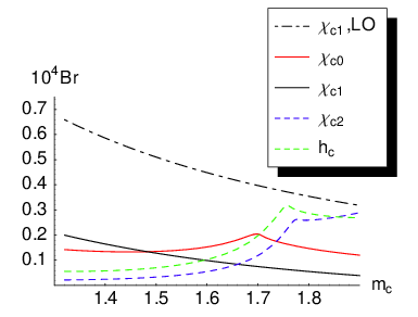
The scale dependence of the NLO result remains significant, simply because the LO term for is canceled, and there is no LO term for the other final states. The scale dependence is exactly of the form for , , and and approximately so for . This causes an uncertainty of a factor of 2 when is varied between GeV and GeV, and larger if one allows smaller scales. However, below about GeV the scale-dependence blows up as seen in the Figure. In the following we fix GeV. Results for other choices of can be obtained approximately by multiplying with . (This remains true, when the spectator-scattering terms are added back.) Other significant parameter dependences arise from the quark mass values. The dependence on is more important than the one on , so we fix GeV in the following. The charm quark mass dependence of the branching fractions, still omitting spectator scattering, is shown in the right plot of Figure 7, from which it is seen that the size of the , branching fractions versus , reverses as increases. The charm quark mass here is the pole mass, which is a poorly defined quantity in perturbation theory, due to large radiative corrections. Typical values are GeV. There may be good reason to choose larger values here, since the charm quark pole mass controls the binding energy , which should be negative in the approximation of charmonium as a non-relativistic bound state, and is negative in reality when measured relative to the threshold. From the Figure it is evident that with the NLO vertex correction alone it is not possible to explain the experimental data, since the , branching fractions are too small, even allowing for theoretical uncertainties in the form factor or the charmonium wave function.

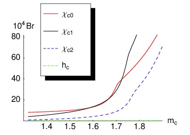
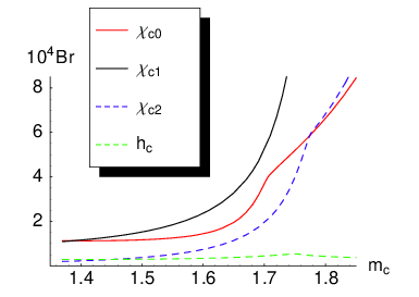
Next we imagine that the branching fractions are given by the spectator-scattering term alone. The largest parameter dependences now arise from the charm quark mass, the Gegenbauer moments of the kaon light-cone distribution amplitude, and the meson distribution amplitude parameter . In Figure 8 we show the dependence for asymptotic distribution amplitudes (left) and for , (right). The branching fractions grow rapidly with , when the spectator amplitude becomes dominated by the imaginary part from the colour-octet contributions. We also observe a huge dependence on the Gegenbauer moments, confirming the expectation that the expansion may be invalid. Even leads to unacceptably large branching fractions. These effects are less pronounced when is larger, since the spectator-scattering branching fraction shown in Figure 8 is proportional to . Independent of these uncertainties, we always find that spectator-scattering is a small effect for , and larger for , than for the other two final states.
| 1.45 | ||||
|---|---|---|---|---|
| 1.50 | ||||
| 1.55 | ||||
| 1.60 | ||||
| 1.65 | ||||
| 1.70 | ||||
| 1.75 |
When we now add both contributions together, including the interference term, we obtain the result shown in Figure 9 for asymptotic distribution amplitudes. For in the range from GeV to GeV, this suggests the interpretation that the , final states are dominated by spectator scattering, more precisely by the spectator-scattering contribution to the colour-octet matrix element. The smallness of the branching fraction is explained by the absence of such a contribution (at leading order) for this final state. The case is intermediate with a rapidly rising branching fraction in the interesting charm-quark mass window. Numerical results for some values of are provided in Table 2. We emphasize that in addition to the charm-quark mass dependence displayed explicitly there are further large theoretical uncertainties related to scale-dependence, which shifts all branching fractions uniformly as described above, to -dependence, to the Gegenbauer moments, and to . There are some parameter degeneracies that allow making and simultaneously larger. In view of these uncertainties the main conclusion of the numerical analysis is that there are reasonable regions of parameter space (GeV, small , and asymptotic kaon distribution amplitude), where the theoretical calculations in our model for the colour-octet matrix elements are in qualitative agreement with the experimental data, namely the existence of large contributions beyond naive factorization, and the suppression of the and modes. From Table 2 we conclude that the small branching fraction is a robust feature of our results, but we find it difficult to explain the strong suppression seen in the data compiled in Table 1, while maintaining the sizeable branching fraction.
6 Conclusion
We revisited exclusive decays to -wave charmonia motivated by previous studies [8, 9, 10, 11, 12, 13] of these decays in the QCD factorization framework that reported a violation of factorization. In contrast, we find that after accounting for colour-octet operators, which, contrary to the case of charmless decays, are not suppressed by due to the existence of the charmonium binding energy scale, QCD factorization is recovered, at least at order . The infrared divergences found in previous calculations can be subtracted consistently into the matrix elements of these operators. This includes the endpoint divergence that is found in the unsubtracted coefficient function associated with spectator-scattering. Our calculations demonstrate that the endpoint contribution, now contained in the colour-octet matrix element, can lead to a large rescattering phase. These observations may be of conceptual interest, since it is presently still unclear in the general case, whether and how endpoint divergences that often appear in convolutions in collinear factorization formulas can be absorbed into well-defined non-perturbative objects and what these objects are. We find it plausible that factorization of decays to -wave charmonium extends to higher orders in the coupling expansion when , in view of the argument presented in [2]; nonetheless, it would be of great interest to verify the factorization of endpoint divergences beyond the tree-approximation to the hard-scattering sub-graph.
Previous numerical estimates of the branching fractions to -waves relied on ad hoc treatments of the infrared regulator dependence. In the present framework, this is unnecessary, but an estimate of the colour-octet operator matrix elements is needed, which may even be the largest contribution to the decay amplitude. To this end we adopted a description of charmonium as a Coulomb bound state, which corresponds to the formal heavy quark limit. In practice, this limit is probably unreliable, and our results do indeed exhibit large theoretical uncertainties. Nevertheless, we find that for plausible theoretical inputs it is possible to reproduce qualitatively what we consider to be the most interesting features of current experimental data: suppression of the and final states and amplitudes that must be dominated by terms beyond naive factorization, though the suppression of is not as strong as observed. An interesting avenue to pursue in the future might be to consider the colour-octet matrix elements as unknown non-perturbative parameters, which is more realistic in view of , and to exploit the constraints imposed by spin-symmetry on the leading contributions to these matrix elements.
Acknowledgement
This work is supported in part by the DFG Sonderforschungsbereich/Transregio 9 “Computergestützte Theoretische Teilchenphysik” and the Swiss National Science Foundation (SNF). M.B. acknowledges hospitality from the University of Zürich and the CERN theory group, where part of this work was performed.
References
- [1] M. Beneke, G. Buchalla, M. Neubert and C. T. Sachrajda, Phys. Rev. Lett. 83, 1914 (1999), [hep-ph/9905312].
- [2] M. Beneke, G. Buchalla, M. Neubert and C. T. Sachrajda, Nucl. Phys. B591, 313 (2000), [hep-ph/0006124].
- [3] C. W. Bauer, D. Pirjol and I. W. Stewart, Phys. Rev. Lett. 87, 201806 (2001), [hep-ph/0107002].
- [4] J. D. Bjorken, Nucl. Phys. Proc. Suppl. 11, 325 (1989).
- [5] J. Chay and C. Kim, hep-ph/0009244.
- [6] H.-Y. Cheng and K.-C. Yang, Phys. Rev. D63, 074011 (2001), [hep-ph/0011179].
- [7] Z.-z. Song, C. Meng and K.-T. Chao, Eur. Phys. J. C36, 365 (2004), [hep-ph/0209257].
- [8] Z.-z. Song and K.-T. Chao, Phys. Lett. B568, 127 (2003), [hep-ph/0206253].
- [9] Z.-Z. Song, C. Meng, Y.-J. Gao and K.-T. Chao, Phys. Rev. D69, 054009 (2004), [hep-ph/0309105].
- [10] T. N. Pham and G.-h. Zhu, Phys. Lett. B619, 313 (2005), [hep-ph/0412428].
- [11] C. Meng, Y.-J. Gao and K.-T. Chao, hep-ph/0502240.
- [12] C. Meng, Y.-J. Gao and K.-T. Chao, hep-ph/0506222.
- [13] C. Meng, Y.-J. Gao and K.-T. Chao, hep-ph/0607221.
- [14] G. T. Bodwin, E. Braaten and G. P. Lepage, Phys. Rev. D46, 1914 (1992), [hep-lat/9205006].
- [15] G. T. Bodwin, E. Braaten, T. C. Yuan and G. P. Lepage, Phys. Rev. D46, 3703 (1992), [hep-ph/9208254].
- [16] M. Beneke, F. Maltoni and I. Z. Rothstein, Phys. Rev. D59, 054003 (1999), [hep-ph/9808360].
- [17] F. Abe et al. [CDF Collaboration], Phys. Rev. Lett. 76, 2015 (1996).
- [18] K. Abe et al. [Belle Collaboration], Phys. Rev. Lett. 88, 031802 (2002), [hep-ex/0111069].
- [19] D. E. Acosta et al. [CDF Collaboration], Phys. Rev. D 66, 052005 (2002).
- [20] F. Fang et al., Phys. Rev. Lett. 90, 071801 (2003), [hep-ex/0208047].
- [21] K. Abe et al. [BELLE Collaboration], Phys. Rev. D 67, 032003 (2003), [hep-ex/0211047].
- [22] B. Aubert et al. [BABAR Collaboration], Phys. Rev. D 69, 071103 (2004), [hep-ex/0310015].
- [23] B. Aubert et al. [BABAR Collaboration], Phys. Rev. D 70, 011101 (2004), [hep-ex/0403007].
- [24] B. Aubert et al. [BABAR Collaboration], Phys. Rev. Lett. 94, 141801 (2005), [hep-ex/0412062].
- [25] B. Aubert et al. [BABAR Collaboration], Phys. Rev. Lett. 94, 171801 (2005), [hep-ex/0501061].
- [26] B. Aubert et al. [BABAR Collaboration], Phys. Rev. D 72, 072003 (2005), [Erratum-ibid. D 74, 099903 (2006)], [hep-ex/0507004].
- [27] B. Aubert et al. [BABAR Collaboration], Phys. Rev. D 72, 051101 (2005), [hep-ex/0507012].
- [28] N. Soni et al. [Belle Collaboration], Phys. Lett. B 634, 155 (2006), [hep-ex/0508032].
- [29] B. Aubert et al. [BABAR Collaboration], Phys. Rev. Lett. 96, 052002 (2006), [hep-ex/0510070].
- [30] B. Aubert et al. [BABAR Collaboration], Phys. Rev. D 74, 032003 (2006), [hep-ex/0605003].
- [31] F. Fang et al., Phys. Rev. D 74, 012007 (2006), [hep-ex/0605007].
- [32] B. Aubert et al. [BABAR Collaboration], Phys. Rev. D 74, 071101 (2006), [hep-ex/0607050].
- [33] B. Aubert et al. [BaBar Collaboration], Phys. Rev. D 76, 092004 (2007), arXiv:0707.1648 [hep-ex].
- [34] E. Barberio et al. [Heavy Flavor Averaging Group], arXiv:0808.1297 [hep-ex], updates at http://www.slac.stanford.edu/xorg/hfag/index.html.
- [35] A. Szczepaniak, E. M. Henley and S. J. Brodsky, Phys. Lett. B243, 287 (1990).
- [36] M. Beneke and T. Feldmann, Nucl. Phys. B592, 3 (2001), [hep-ph/0008255].
- [37] C. Bobeth, B. Grinstein and M. Savrov, Phys. Rev. D77, 074007 (2008), arXiv:0712.1953 [hep-ph].
- [38] G. T. Bodwin, X. Garcia i Tormo and J. Lee, arXiv:0805.3876 [hep-ph].
- [39] B. Melic, Phys. Rev. D 68, 034004 (2003), [hep-ph/0303250].
- [40] Z. G. Wang, L. Li and T. Huang, Phys. Rev. D 70, 074006 (2004), [hep-ph/0311296].
- [41] B. Melic, Phys. Lett. B 591, 91 (2004), [hep-ph/0404003].
- [42] J. Chay and C. Kim, Nucl. Phys. B680, 302 (2004), [hep-ph/0301262].
- [43] C. W. Bauer, D. Pirjol, I. Z. Rothstein and I. W. Stewart, Phys. Rev. D70, 054015 (2004), [hep-ph/0401188].
- [44] M. Beneke and S. Jäger, Nucl. Phys. B751, 160 (2006), [hep-ph/0512351].
- [45] M. Beneke and D. Yang, Nucl. Phys. B736, 34 (2006), [hep-ph/0508250].
- [46] M. Beneke and T. Feldmann, Nucl. Phys. B685, 249 (2004), [hep-ph/0311335].
- [47] M. Beneke, G. A. Schuler and S. Wolf, Phys. Rev. D62, 034004 (2000), [hep-ph/0001062].
- [48] M. Beneke, Y. Kiyo and A. A. Penin, Phys. Lett. B653, 53 (2007), [0706.2733].
- [49] M. Beneke and Y. Kiyo, Phys. Lett. B 668, 143 (2008), [0804.4004].
- [50] T. Becher, R. J. Hill and M. Neubert, Phys. Rev. D69, 054017 (2004), [hep-ph/0308122].
- [51] A. V. Manohar and I. W. Stewart, Phys. Rev. D76, 074002 (2007), [hep-ph/0605001].
- [52] G. Bell and T. Feldmann, Nucl. Phys. Proc. Suppl. 164, 189 (2007), [hep-ph/0509347].
- [53] E. Bagan, P. Ball and V. M. Braun, Phys. Lett. B 417, 154 (1998), [hep-ph/9709243].
- [54] C. M. Arnesen, Z. Ligeti, I. Z. Rothstein and I. W. Stewart, Phys. Rev. D77, 054006 (2008), [hep-ph/0607001].
- [55] Quarkonium Working Group, N. Brambilla et al., hep-ph/0412158.
- [56] P. Ball and R. Zwicky, Phys. Rev. D71, 014015 (2005), [hep-ph/0406232].
- [57] A. Khodjamirian, T. Mannel and M. Melcher, Phys. Rev. D 70 (2004) 094002, [hep-ph/0407226].
- [58] V. M. Braun and A. Lenz, Phys. Rev. D 70 (2004) 074020, [hep-ph/0407282].
- [59] P. Ball and R. Zwicky, Phys. Lett. B 633 (2006) 289, [hep-ph/0510338].
- [60] P. Ball, V. M. Braun and A. Lenz, JHEP 0605 (2006) 004, [hep-ph/0603063].
- [61] V. M. Braun et al., Phys. Rev. D 74 (2006) 074501, [hep-lat/0606012].
- [62] P. A. Boyle et al. [UKQCD Collaboration], Phys. Lett. B 641 (2006) 67, [hep-lat/0607018].