Temperature effect on the power spectrum in inflation

The scenario of the inflation provides an excellent solution to the horizon and flatness problems [1]. During inflation the quantum fluctuations in the inflaton field can freeze out and become the seed for large scale structure [2, 3]. These fluctuations can translate into perturbations in energy density and curvature in the universe and can be imprinted in the anisotropy of cosmic microwave background (CMB), which can be measured with higher and higher precision nowadays. Recently an intriguing possibility has been discovered in the literature that inflation might provide a window towards physics beyond the Planck scale [4, 5, 6, 9, 10, 7, 8, 11, 12]. Chances to detect such trans-Planckian effect in the CMB observation have been addressed in Refs.[9, 10, 7, 8].

In the standard inflationary scenario, initial conditions for the inflaton field are imposed in the infinite past with an infinitely short wavelength when the effect of the inflationary horizon and the expansion of the universe can be ignored. The spacetime is essentially Minkowskian and there is a unique vacuum, the Bunch-Davis vacuum, for the inflaton field. To encode the new physics near the Planck scale, a simple modification in the standard scenario has been focused on different choices of the vacuum [12, 13, 14, 15, 16, 17, 18, 19, 20, 21, 22]. It has been shown that based on some choices of vacua discussions of many trans-Planckian effects can be carried out and qualitative correction due to Planck scale can be obtained without detailed knowledge of trans-Planckian physics. However, all these vacua chosen to discuss the inflation are of zero temperature.

Inflation started just shortly after the big bang when the universe was extremely hot at that moment. Before the inflation it would be reasonable to consider that the universe was in thermal equilibrium. After the inflation, the thermal equilibrium can be restored. In the process of the inflation, the inflaton coupled extremely weak to thermal fields so that the inflaton itself is out of the thermal equilibrium during inflation. However, considering that the inflation process is extremely short, one can suppose that this process can be described with the comoving temperature $\tilde{T}=Ta$ to relate the initial and final states [23, 24], where $a$ is the scale factor, and use the thermal ground state for the inflaton. In our work we will use this assumption and employ the thermo field dynamics to discuss the problem in detail.

In thermo field dynamics [25], suppose the temperature of the form $T=1/\beta$, the Bogoliubov transformations of the usual boson operators

can be reversed into

where $\cosh\theta_{k}=\frac{1}{\sqrt{1-e^{-\beta\omega(k)}}}$, $\sinh\theta_{k}=\frac{e^{-\beta\omega(k)}}{\sqrt{1-e^{-\beta\omega(k)}}}$ and spectrum $\omega(k)=\sqrt{p^{2}+m^{2}}=\sqrt{k^{2}/a^{2}+m^{2}}$. Obviously $\cosh\theta_{k}=\cosh\theta_{-k}$ and $\sinh\theta_{k}=\sinh\theta_{-k}$, then in the following we will simply use $\theta_{k}$.

In above definition we introduced the tilde operators $\hat{\tilde{a}}_{k}$ and $\hat{\tilde{a}}^{\dagger}_{k}$ in the duplicated space in additional to the normal operators. Correspondingly, the state space should also be doubled, which means that we will not only have $|n\rangle$, but also $|\widetilde{n}\rangle$ ($n=0,1,2,\cdots$). The tilde operators operate on tilde space vector $|\widetilde{n}\rangle$ while the normal operators operate on the normal state $|n\rangle$. Thermal operators satisfy the commuting relations, $[\hat{a}_{k}(\beta),\hat{a}^{\dagger}_{k}(\beta)]=1$, $[\hat{\tilde{a}}_{k}(\beta),\hat{\tilde{a}}^{\dagger}_{k}(\beta)]=1$, $[\hat{a}_{k}(\beta),\hat{\tilde{a}}_{k}(\beta)]=0$, which can be verified directly from the commutators of the operators $\hat{a}_{k}$ and $\hat{\tilde{a}}_{k}$.

Now we express the thermal vacuum as $|\beta 0\rangle$. From the thermo field dynamics, we learn that thermal vacuum state of a boson field is the infinite linear composition of the state $|n,\widetilde{n}\rangle$:

which satisfies

With these formalism, we are in a position to examine the influence of the thermal vacuum on the power spectrum of the inflation.

In zero temperature case, given a statefunction $\chi_{k}$ solved from field equation in momentum space, we can build up the field operator as

In the scalar perturbation, the power spectrum is defined as [3]

where the last factor arises from the expectation value of the field operator in the vacuum state,

In the thermal vacuum, the field operator $\hat{\chi}$ can be expressed as

by substituting Eq.(2) into Eq.(5). We see now the field space is composed of two parts, the normal space and the duplicate space, with weights $\cosh\theta_{k}$ and $\sinh\theta_{k}$, respectively.

The particle number can be calculated as

which is just the distribution of thermal equilibrium states.

The power spectrum of perturbation in the thermal vacuum becomes

where $P_{k}$ is the power spectrum obtained by considering the zero temperature vacuum. For the massless scalar field, $\omega=p=k/a$. The temperature effect appears in the factor $\coth\frac{k}{2aT}$, which shows that the power spectrum gets modified due to the thermal effect. When $T\rightarrow 0$, Eq.(10) reduces to the usual result of Eq.(6). In the above derivation, we use the finite temperature field theory which clearly shows the temperature effect in the vacuum. This approach is general and does not depend on the choice of the vacuum.

Adding the thermal effect in the adiabatic vacuum, we can generalize the power spectrum in [6] by including the thermal factor as

where $\tilde{T}=aT$ is the comoving temperature and $\Lambda$ is the trans-Planckian energy level. The second term in the bracket represents the effect brought by the trans-Planckian physics. At zero temperature the modulation of the power spectrum of primordial density fluctuation predicted in the trans-Planckian model has been studied by considering the change of the Hubble parameter and slow-roll condition [26]

where $M_{PL}^{-2}=8\pi G$ is the reduced Planck mass. In Ref.[26], adopting the scale parameter $\gamma=\Lambda/M_{PL}$ and $H/\Lambda=\xi(k/k_{0})^{-\varepsilon}$, the trans-Planckian power spectrum is expressed into

where $\xi\approx 4\times 10^{-4}\sqrt{\varepsilon}/\gamma$ and the pivot scale $k_{0}=0.05$ Mpc${}^{-1}\approx 213.8H_{0}$, based on the value $H_{0}=70.1$ km s^-1 Mpc^-1 from five-year WMAP result [27]. The power spectra $P(k)$ for different values of $\gamma$ and $\varepsilon$ were shown in Ref.[26]. In Fig.1 we illustrate their result of zero temperature case in the solid line by taking $\varepsilon=\gamma=0.01$.

Considering the thermal effect with additional term $\coth\frac{k}{2\tilde{T}}$, we have the power spectrum

The temperature influence on the power spectrum $P_{k}$ is shown by the dashed line in Fig.1. We took $\tilde{T}=H_{0}$ in our plot and noticed that different values of $\tilde{T}$ will not change the qualitative behavior of the dashed line. The thermal influence becomes significant especially at small $k$, while its influence can be neglected for big enough $k$. In other words the change in the spectrum due to the thermal effect is large at large angles and small at small angles. This brings an interesting possibility that the thermal effect might influence the CMB at small $l$.

When $k\rightarrow 0$, because of the factor $\coth\frac{k}{2\tilde{T}}$, we will meet the divergence problem in the power spectrum, which is unphysical. To tackle this problem we resort to the idea of the holographic cutoff employed in [28, 29]. Relating the ultraviolet and infrared cutoff [30], the quantum zero-point energy density $\rho_{\Lambda}$ which can be related to the cosmological constant or dark energy density in a flat universe can be expressed by

where $L$ is the infrared cutoff, and $c$ is a constant parameter. From this relation, we can write $L=c/(\sqrt{\Omega_{\Lambda 0}}H_{0})$, where $\Omega_{\Lambda 0}$ is the present value of the dark energy ratio to the critical density $\Omega_{\Lambda}=\rho_{\Lambda}/\rho_{cr}=\rho_{\Lambda}/(3M_{PL}^{2}H^{2})$. Consequently this introduces the cutoff at the wave number [29]

This holographic cutoff can help to remove the divergency brought by $k=0$.

Now we move on to examine the thermal effect on the CMB at small $l$ by comparing with the WMAP data. The CMB angular spectrum is expressed as [31]

where $j_{l}$ is the spherical Bessel function and $\Delta\tau$ is the comoving distance to the last scattering surface,

and $z_{0}$ is the redshift of decoupling usually taken as $z_{0}=1100$. We choose the Hubble parameter

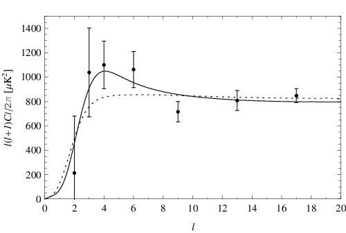
where $w=p/\rho$ is the equation of state of dark energy and is assumed as a constant for simplicity. In our numerical calculation, we will set $\Omega_{\Lambda 0}=0.721$ and $w=-0.972$ [27]. For the zero temperature case, it has been shown that the relation between ultraviolet and infrared cutoff can help to explain the small $l$ CMB suppression [29], which is exhibited in the dashed curve in Fig.2. However, compared with the WMAP data, it cannot explain well the wriggle observed at $l=3,4,6$.

Notice that the thermal effect may play the role at large angle to modify the power spectrum, we now turn to the temperature dependent spectrum in Eq.(14). To do the data fitting with WMAP result at small $l$, we have parameters $\tilde{T}$, $c$, $\varepsilon$ and $\xi$ or $\gamma$ now. We observed that in the reasonable range of slow-roll condition, values of $\varepsilon$ and $\gamma$ do not significantly change the total power spectrum, thus we fix them to be $\varepsilon=0.03$ and $\gamma=0.003$ to ensure observable trans-Planckian effect to be found in CMB [26]. Now we have two parameters $c$ and $\tilde{T}$ to be determined. Calculating the angular power spectrum $l(l+1)C_{l}$ and comparing with WMAP data by doing $\chi^{2}$ fitting for $0<l\leq 20$,

where $\sigma^{i}$ is the observational error of each data, we present the best fitting result in solid line in Fig.2, where $c=2.5$ and $\tilde{T}=0.9H_{0}\approx 1.3\times 10^{-33}$ eV $\approx 1.6\times 10^{-29}$ K. This result keeps almost the same when we shift $\varepsilon$ and $\gamma$ in the reasonable range of the slow-roll inflation condition. It can be seen from Fig.2 that the thermal effect can well explain the WMAP data at small $l$, especially the wriggle at $l=3,4,6$.

In summary, we have employed the thermo field dynamics to investigate the thermal vacuum effect on the power spectrum of the inflation. Comparing with the spectrum of the zero temperature case, we have observed that the thermal effect plays the role essentially in the low multipoles or large length scale. Resorting to the idea of holographic cutoff, we have removed the divergence problem when $k=0$. Comparing with the WMAP data at small $l$, we have found that the thermal effect explains well the data at small $l$ than the zero temperature case. When $l=3,4,6$, the spectrum got enhanced due to the temperature effect. This suggests that the thermal effect should be considered in studying the inflation, especially when we want to study the CMB anisotropy at low multipoles. The temperature was very high at the beginning of the inflation, so it actually influences the fluctuation spectrum which escaped earlier from the horizon and reentered later so that the large scale (small $l$) CMB spectrum got corrected. When the inflation started, the temperature dropped fast, and the temperature effect has less influence on the fluctuation spectrum. These fluctuations left the horizon later and reentered earlier which affect the small scale CMB spectrum. Since the temperature effect is low, most CMB spectrum ($l>10$) has little difference compared with the zero temperature case. This actually gives the reason why we see the temperature correction is important in the small $l$ CMB spectrum, which is consistent with the observation, while for big $l$, the temperature effect is negligible.

References

- [1] A. H. Guth, Phys. Rev. D 23, 347 (1981).
- [2] A. Linde, Particle Physics and Inflationary Cosmology (Harwood Academic, Chur, Switzerland, 1990), arXiv:hep-th/0503203.
- [3] A.R. Liddle and D.H. Lyth, Cosmological Inflation and Large- Scale Structure (Cambridge University Press, Cambridge, England, 2000).
- [4] R. Easther, B. R. Greene, W. H. Kinney, and G. Shiu, Phys. Rev. D 64, 103502 (2001).
- [5] R. Easther, B. R. Greene, W. H. Kinney, and G. Shiu, Phys. Rev. D 66, 023518 (2002).
- [6] U. F. Danielsson, Phys. Rev. D 66, 023511 (2002).
- [7] N. E. Groeneboom and Østein Elgarøy, Phys. Rev. D 77, 043522 (2008).
- [8] J. Ren, H.-G. Zhang, and X.-H. Meng, arXiv:astro-ph/0612011v2.
- [9] J. Martin and C. Ringeval, Phys. Rev. D 69, 083515 (2004); ibid. 127303 (2004).
- [10] J. Martin and C. Ringeval, J. Cosmol. Astropart. Phys. 01 (2005) 007; ibid. 08 (2006) 009.
- [11] B. Wang, L. H. Xue, Z. Zhang, and W-Y. P Hwang, Phys. Rev. D 67, 123519 (2003).
- [12] K. Goldstein and D. A. Lowe, Phys. Rev. D 67, 063502 (2003).
- [13] U. H. Danielsson, J. High Energy Phys. 12 (2002) 025.
- [14] R. H. Brandenberger, hep-th/0210186.
- [15] X. Wang, B. Feng, and M. Li, Int. J. Mod. Phys. D14, 1347 (2005).
- [16] C. P. Burgess, J. M. Cline, F. Lemieux, and R. Holman, J. High Energy Phys. 02 (2003) 048.
- [17] N. A. Chernikov and E. A. Tagirov, Ann. Inst. Henri Poincaré, vol. IX, 2 (1968) 109.
- [18] E. Mottola, Phys. Rev. D 31, 754 (1985).
- [19] B. Allen, Phys. Rev. D 32, 3136 (1985).
- [20] R. Floreanini, C. T. Hill, and R. Jackiw, Ann. Phys. (NY) 175, 345 (1987).
- [21] R. Bousso, A. Maloney, and A. Strominger, Phys. Rev. D 65, 104039 (2002).
- [22] M. Spradlin and A. Volovich, Phys. Rev. D 65, 104037 (2002).
- [23] A. H. Guth and S.-Y. Pi, Phys. Rev. D 32, 1899 (1985).
- [24] K. Bhattacharya, S. Mohanty, and R. Rangarajan, Phys. Rev. Lett. 96, 121302 (2006); ibid. 97, 231301 (2006).
- [25] H. Umezawa, H. Matsumoto, and M. Tachiki. Thermo field dynamics and condensed states (North-Holland, Amsterdam, 1982).
- [26] L. Bergström and U. F. Danielsson, J. High Eenergy Phys. 12 (2002) 038.
- [27] G. Hinshaw, et al., arXiv:0803.0732.
- [28] K. Enqvist, M. S. Sloth, Phys. Lett. 93 (2004) 221302; K. Enqvist, S. Hannestad, and M. S. Sloth, astro-ph/0409275.
- [29] J. Shen, B. Wang, E. Abdalla, and R.-K. Su, Phys. Lett. B609 (2005) 200; Z.Y. Huang, B. Wang, E. Abdalla, R.K. Su, JCAP 0605 (2006) 013.
- [30] A. G. Cohen, A. B. Kaplan, and A. E. Nelson, Phys. rev. Lett 82, 4971 (1999).
- [31] M. Giovanini, Int. J. Mod. Phys. D14 363, (2005).