Diagnostics of the Early Explosion Phase of a Classical Nova Using Its X-ray Emission: A Model for the X-ray Outburst of CI Camelopardalis in 1998
Abstract
We have computed a spherically symmetric model for the interaction of matter ejected during the outburst of a classical nova with the stellar wind from its optical component.This model is used to describe the intense X-ray outburst (the peak 3-20 keV flux was 2 Crab) of the binary system CI Camelopardalis in 1998. According to our model, the stellar wind from the optical component heated by a strong shock wave produced when matter is ejected from the white dwarf as the result of a thermonuclear explosion on its surface is the emission source in the standard X-ray band. Comparison of the calculated and observed time dependences of the mean radiation temperature and luminosity of the binary system during its outburst has yielded very important characteristics of the explosion.We have been able to measure the velocity of the ejected matter immediately after the onset of the explosion for the first time: it follows from our model that the ejected matter had a velocity of 2700 km/s even on 0.1-0.5 day after the outburst onset and it flew with such a velocity for the first 1-1.5 day under an external force, possibly, the radiation pressure from the white dwarf. Subsequently, the matter probably became transparent and began to decelerate. The time dependence of the mean radiation temperature at late expansion phases has allowed us to estimate the mass of the ejected matter, . The mass loss rate in the stellar wind required to explain the observed peak luminosity of the binary system during its outburst has been estimated to be .
Key Words.
classical novae – X-ray emission – numerical calculations1 Introduction
1.1 X-ray Emission During Classical Nova Outbursts
Explosive thermonuclear burning of matter on the surface of a white dwarf is generally believed to be responsible for the phenomenon of classical novae (see, e.g., the review by Gallagher and Starrfield (1978)). During a thermonuclear runaway, a large mass accreted on the white dwarf surface (up to , Prialnik and Kovetz 2005) is ejected and accelerated to high velocities, km/s (see, e.g., Prialnik 1986; Prialnik and Kovetz 2005).
At the initial evolutionary phases of a nova outburst, a high mass loss rate of the white dwarf envelope causes the effective photosphere of the envelope to increase in size up to cm, depending on the energy band (see, e.g., Kato and Hachisu 1994). Subsequently, the photospheric radius decreases over several months, because the envelope gradually becomes optically thin, until the entire envelope becomes completely transparent to emission.
At this evolutionary phase of a classical nova, the on-going hydrogen burning on the surface of the white dwarf temporarily turns it to the so-called "supersoft" X-ray source (see, e.g.,MacDonald et al. 1985; Kahabka and van den Heuvel 1997) - the entire surface of the white dwarf produces a flux that is approximately equal to the Eddington one. In an optically thick regime and at typical white dwarf sizes, cm, the latter corresponds to a blackbody temperature of about 20-50 eV.
Classical and recurrent (i.e., erupting several times, e.g., Nova RS Oph) novae can also be the sources of standard ( keV) and hard ( keV) X-ray emission. The most popular model for the generation of such emission is the shock model.
In the external shock model, a dense envelope that rose from the white dwarf surface as a result of the explosion and that was accelerated to velocities km/s produces a strong shock wave in the stellar wind from the companion star. The shock-heated wind matter is the source of X-ray emission up to energies 5-80 keV (). For example, the described mechanism is believed to be responsible for the generation of hard X-ray emission from the recurrent Nova RS Oph (see, e.g., Bode and Kahn 1985; O’Brien et al.1992; Sokoloski et al.2006).
Evidently, the external shock model is naturally linked to the existence of a dense medium near the binary system; otherwise, the emission measure of the shock-heated plasma ( ) would not be enough to provide the necessary (observed) X-ray luminosity. However, in most cases, the companions in classical novae are unevolved main-sequence stars (Bath and Shaviv 1978) whose weak stellar wind is unable to produce a dense medium near the binary system needed for the external shock model.
In the internal shock model, the ejected envelope has a velocity gradient as a result of which the faster inner layers catch up with the slower outer ones to produce a shock wave inside the expanding envelope (Lloyd et al.1992; O’Brien et al.1994; Mukai and Ishida 2001).The internal shock model was successfully applied to such classical novae as Nova Herculis 1991 (Lloyd et al.1992) and Nova Velorum 1999 (Mukai and Ishida 2001).
The internal and external shock models are not mutually exclusive and can make comparable contributions to the total X-ray emission from the nova under certain conditions.The most important factor here is the acceleration law of the ejected envelope (here, we discuss only the initial evolutionary phase of the nova) and the density of the stellar wind from the companion star. It is possible that not all of the envelope matter is instantaneously accelerated to the velocities measured at later envelope expansion phases from the parameters of optical and infrared emission lines (see, e.g., Hynes et al. 2002; Das et al. 2006). Therefore, the inner layers of the envelope can have higher outflow velocities and, hence, an internal shock that affects significantly the observational manifestations of the nova in X-rays can be generated inside the ejected envelope irrespective of the efficiency of the external shock model.
The envelope acceleration process is important not only in explaining the X-ray emission from the nova, but it is also fundamentally important in understanding the physical processes in the burning envelope of the white dwarf. Thus, for example, the enrichment of the envelope with white dwarf matter (mainly carbon and oxygen) is very important for the formation of a rapidly expanding envelope in actual nova explosions. The energy release in the white dwarf envelope through thermonuclear burning computed in 1D numerical simulations with convective motions described by the mixing-length theory allows high envelope expansion velocities to be obtained (see, e.g., Starrfield et al.1985; Prialnik 1986; Yaron et al., 2005). However, more detailed 2D and 3D burning calculations do not allow such high velocities to be obtained without the assumptions about greatly enhanced carbon and oxygen abundances in the envelope (Kercek et al.1998; Glasner et al. 2005, 2007). Measuring the envelope expansion law would be the most important observational test of the white dwarf envelope burning model.
The expansion law of the envelope ejected from the white dwarf is exceptionally difficult to test, because this process takes place within the first hours or even minutes after the onset of explosive thermonuclear burning, i.e., long before the maximum optical light of the nova, i.e., in fact, before its actual detection in astronomical observations. The observations of hard X-ray emission from several classical novae a few days after their maximum light in the optical energy band are not enough for this.
Only recently has a unique opportunity arisen to test the nova envelope expansion models using the X-ray emission from one of the most unusual transients in the X-ray sky, XTE J0421+560/CI Cam, as an example.
1.2 XTE J0421+560/CI Cam


The source XTE J0421+560 (later identified with the well-known variable star CI Cam; Wagner and Starrfield 1998) was discovered as an X-ray transient on March 31, 1998 (Smith et al. 1998). The flux from the source rose to 2 Crab in several hours. Subsequent observations of the system revealed a variable flux in both optical and radio bands (see, e.g., Clark et al. 2000).
The properties of XTE J0421+560 differed strikingly from those of ordinary X-ray transients (see, e.g., Tanaka and Shibazaki 1996). Various emission lines typical of the emission from an optically thin plasma with a temperature of 1-10 keV (Orr et al. 1998; Ueda et al. 1998; Revnivtsev et al. 1999) but absolutely atypical of the emission from bright X-ray transients were detected in its spectrum.
It was also found that, in contrast to ordinary X-ray transients (accreting neutron stars and black holes), the flux from XTE J0421+560 was highly stable at all Fourier frequencies - apart from a general decline in flux, only an upper limit on the variability of the source’s X-ray flux on time scales of 20-1000 s could be obtained (Revnivtsev et al. 1999).
Subsequent studies of the source’s behavior at late evolutionary phases (Ishida et al.2004), in quiescence (Boirin et al.2002), and investigation of the evolution of the radio emission from the 1998 outburst (Mioduszewski and Rupen 2004) suggested that the intense 1998 outburst was the explosion of a classical nova in the binary system CI Cam and the compact object in XTE J0421+560 is most likely an accreting white dwarf.
For a classical nova, the X-ray emission from XTE J0421+560 during the 1998 outburst is extraordinarily intense. For comparison, the peak X-ray flux from the widely known recurrent Nova RS Ophiuchi (Sokoloski et al.2006; Bode et al. 2006) was a factor of 10-30 lower than that from CI Cam during its 1998 outburst. A strong stellar wind from the optical component in the binary system, a B[e] giant star (Hynes et al.2002; Barsukova et al.2006; Robinson et al.2002), is responsible for such a high luminosity of the CI Cam/XTE J0421+560 outburst (we will show this below). It is the presence of such a dense medium around the expanding envelope of the nova that produced the necessary emission measure ( ) of the shock-heated plasma.
The assumption that the explosion of a classical nova is responsible for the giant X-ray outburst of XTE J0421+560/CI Cam in 1998, along with the high X-ray intensity of the transient (the peak flux from the source reached 2 Crab), which allowed a large set of high-quality observational data covering almost the entire evolution of the transient’s X-ray outburst to be obtained, provides an excellent opportunity to test the most important ingredients of the external shock model for classical nova explosions.A unique feature of the set of XTE J0421+560/CI Cam observations from the standpoint of studying the evolution of the classical nova envelope expansion is the transient’s light curve obtained by the All-Sky Monitor (ASM) of the RXTE observatory half a day before the X-ray flux peak. It allows the motion of the expanding envelope to be “seen” starting from several hundred white dwarf radii ( cm). The evolution of the X-ray outburst of XTE J0421+560, which, on the whole, lasted about 10 days, was well covered by RXTE observations (Revnivtsev et al. 1999). This also makes it possible to compare the predictions of the shock models during the decline in X-ray flux.
This paper is the first in a series of papers that investigate the behavior of the X-ray emission from CI Cam using hydrodynamic simulations of the expansion of the white dwarf envelope and its interaction with the stellar wind from the companion star.
The goal of this paper is to demonstrate that the main features of the X-ray outburst of CI Cam can be explained in terms of the model of a shock wave passing through the stellar wind during a classical nova explosion.We investigated in detail the following important points of the explosion:
- •
the envelope motion at the initial expansion stages after the explosion;
- •
the deceleration of the envelope as it interacts with the stellar wind;
- •
the contribution from radiative cooling to the change in the temperature of the stellar wind from the companion passed through the shock wave.
1.3 Basic Characteristics of the Emission from CI Cam During the 1998 Outburst
During the giant outburst of CI Cam in 1998, the X-ray emission from this binary system had several characteristic features that, as we will show below, can be explained in terms of the model of emission generation as the shock wave produced by the expanding envelope of the white dwarf passes through the stellar wind from the optical companion.
- •
At the rise phase of the light curve, the time dependence of the source’s 3-20 keV luminosity was (Fig.1, left).
- •
The peak luminosity of the source was erg/s, where d is the distance to the source.
- •
The mean (effective) radiation temperature of the source was constant and equal to kT 10 keV for 2 days from the outburst onset (Fig.1, right).
- •
After the second day from the outburst onset, the radiation temperature decreased approximately as .
2 The Method Of Numerical Calculations
2.1 The Computational Scheme
In this paper, we used numerical hydrodynamic calculations to derive the time dependences of the effective temperature and X-ray luminosity of a classical nova.
In our calculations, we used a 1D spherically symmetric code in Lagrangian coordinates with a staggered mesh (the cell radius, velocity, and mass are determined at the cell boundaries, while the density, pressure, and internal energy are determined at the cell mass centers). A more detailed description of this computational scheme can be found in Janka et al. (1993).
We disregarded the gravitational attraction from the white dwarf, since the shock wave in our calculations is generated at a distance, cm, at which the escape velocity from the white dwarf, 230 km/s, is much lower than the envelope velocity, 3000 km/s. We also disregarded the influence of the optical star on the shock propagation.
2.2 Radiative Cooling and Thermal Instability

In our calculations, we took into account the radiative cooling of the stellar wind matter from the optical companion passed through the shock wave. The bremsstrahlung of an optically thin plasma was assumed to be the main mechanism of the radiative losses.We calculated the rate of plasma energy losses through radiation using the APEC model (http://hea-www.harvard.edu/APEC/REF) by assuming that ionization equilibrium was established instantly in the heated matter. The derived cooling functions are shown in Fig.2. For convenience, these functions were reduced to the total particle number density. The cosmic abundances were taken from Grevesse and Sauval (1998), the mean molecular weight of the plasma particles at such abundances is , and , where is the total number of particles. To take into account the radiative energy losses, we used the 0.01-50 keV energy band in our calculations, which is sufficient for the temperatures expected in our model. The 3-20 keV energy band was used to construct the model light curves.
A simple estimate of the stellar wind density at which radiative cooling begins to affect significantly the thermal balance of the post-shock matter can be obtained by comparing the radiative cooling time through bremsstrahlung alone with the characteristic times in our problem, several days. For our estimate, we will take 1 day. The gas in our calculations was assumed to be ideal with the adiabatic index :
where is the temperature of the emitting plasma, is the total density of the stellar wind matter passed through the shock wave, and is the plasma emissivity (cooling function). For the observed temperature, kT 10 keV, the plasma emissivity is and a radiative cooling time of 1 day corresponds to an unperturbed stellar wind density .
In the case where the radiative cooling time of the shock-heated matter is shorter than the characteristic time of its expansion (several days), an isobaric thermal instability develops (see, e.g., Field 1965). In 1D calculations, this leads to a number of nonphysical effects. However, since the matter cooled below a temperature of 1 keV ceases to radiate in the energy band of interest to us (3-20 keV), its specific temperature does not affect the results of our calculations as long as the thermal instability develops at constant pressure. Therefore, when the cell cooling time was less than 0.1 day (which corresponds to temperatures 0.9 keV at typical densities in our problem), we switched off the cooling in this cell and, at the same time, excluded its emission from our calculations of the observed X-ray luminosity and the mean temperature of the X-ray emission.
Let us now show that our approximation of the instant establishment of ionization equilibrium downstream of the shock is valid. Before estimating the time it takes for ionization equilibrium to be established, we must calculate the time it takes for a Maxwellian ion velocity distribution to be established and the equipartition time of the post-shock ion and electron temperatures , since the shock wave heats only the ions. Spitzer et al.(1965) showed that
where and are the ion and electron temperatures in kelvins, is the ion density, is the atomic weight of the electron, is the atomic weight of the ion, and is the Coulomb logarithm.
For our estimates, we will take and . Then,
where . The time it takes for the electron temperature to be established is s.
To estimate the time it takes for ionization equilibrium to be established downstream of the shock, we will use a formula from Masai (1994):
where is the electron density. It follows from our estimates that the longest time it takes for the temperature to be established () and the time it takes for ionization equilibrium to be established () downstream of the shock are much shorter than the radiative cooling time of the matter ( day) at the same density (here, ). Hence, our approximation of the instant establishment of ionization equilibrium downstream of the shock is valid. We also see from our estimates that the shock at matter parameters typical of our problem is not radiative (since ), i.e., the density jump at the shock is defined by the formula and is for our value of .
2.3 Calculating the Mean Temperature of the X-ray Emission

Below, we will show that, in general, the post-shock stellar wind matter is a multi-temperature plasma. Consequently, the radiation temperature that we measure based on X-ray observations is an average and it may not be equal to the temperature at the shock front. Ttherefore, to obtain the calculated mean temperature, we used the same averaging procedure as that for the observations. We calculated the ratio of the 3-5 and 5-20 keV fluxes, which, in turn, corresponds to a certain temperature in the radiation model of a single-temperature optically thin plasma. The flux ratio in the model of a single-temperature plasma was calculated using the APEC model. The efficiency of the method is shown in Fig. 3, where the solid line indicates the combined spectrum of the post-shock matter at some instant of time and the dashed line indicates the spectrum of a single temperature plasma with the temperature determined by the method described above. We see from Fig. 3 that the method is efficient in our case.
2.4 Initial Conditions
The stellar wind density, temperature, and velocity profiles were specified in our calculations as the initial conditions. The first inner cell of the computational grid with a finite mass was specified as the piston- envelope. This allowed us to subsequently consider the influence of the piston envelope mass on the shock dynamics.
In our calculations with the piston-envelope, the initial cell size was cm. The inner boundary of the computational grid was placed at cm. We performed calculations with various initial grid cell sizes to ascertain the optimal computational time/accuracy ratio.An increase in the resolution by a factor of 10 caused a change in the mean temperature of the emitting matter by a few percent while increasing significantly the computational time.
In our case, the stellar wind temperature does not affect the shock generation; therefore, it was taken to be approximately equal to the effective temperature of the optical star, eV. The temperature of the piston-envelope was taken to be equal to that of the stellar wind.
Since the stellar wind velocity (35 km/s; Robinson et al.2002) is low compared to the envelope velocity (1000-4000 km/s) and does not affect the shock generation either, it was set equal to zero in our calculations for simplicity.
For the models with a constant envelope expansion velocity, constant velocities were maintained at both boundaries of the envelope cell.
When the shock wave was modeled in the Sedov regime (a strong point explosion in a spherically symmetric medium), the internal energy of the first four cells increased to the necessary explosion energy, whereupon the system relaxed. For our calculations in this regime, we set the initial cell size equal to cm.
3 Positions Of The Components In CI Cam At The Time Of Its Outburst
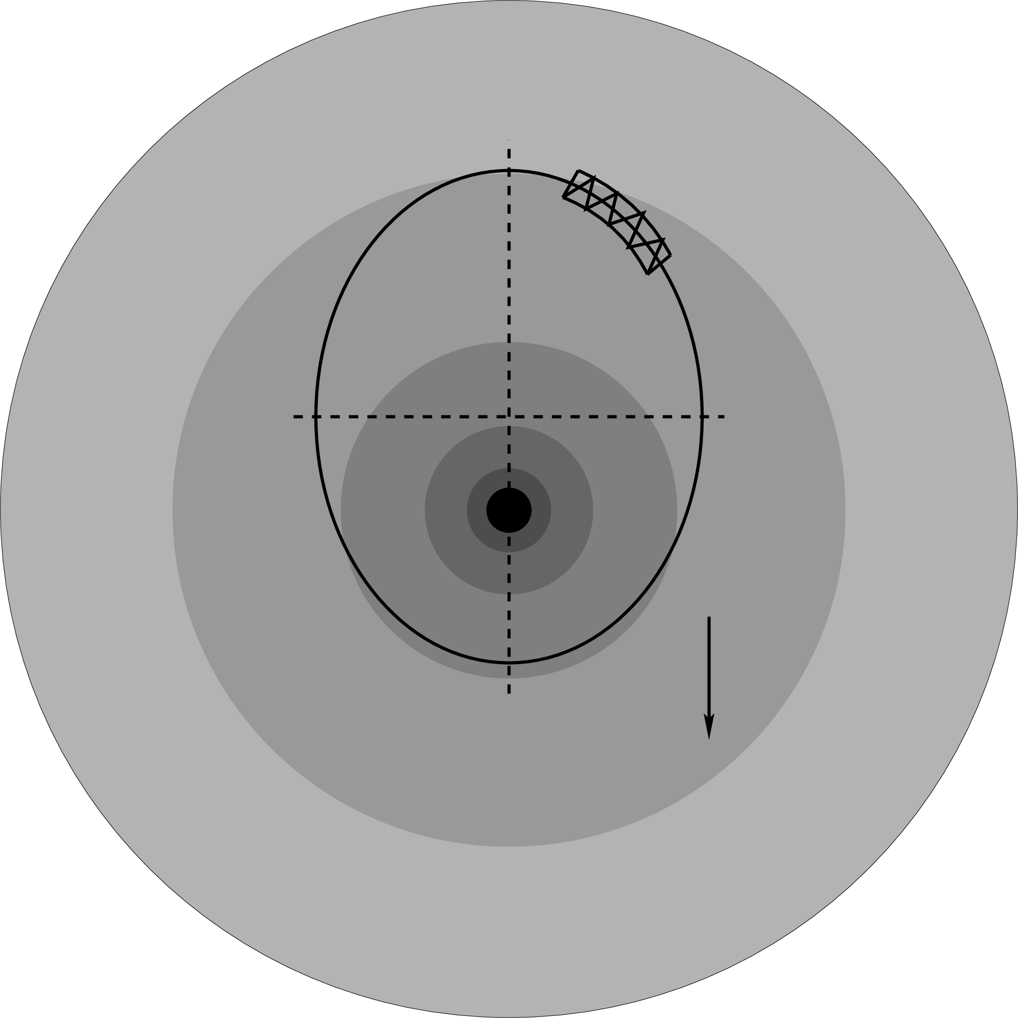
The optical component in the binary system CI Cam is an early B[e] star (Hynes et al.2002; Barsukova et al.2006), presumably a B4 III-V giant (Barsukova et al. 2006). The radius of the optical component is cm.
If the star is a supergiant (see, e.g., Hynes et al. 2002; Robinson et al. 2002), then its radius is considerably larger and can reach cm. The orbital parameters of the binary were determined by Barsukova et al. (2006): its orbital period is days, the semi-major axis of its orbit is cm (here, is the inclination of the binary), and its eccentricity is . The distance to the binary system is not yet known accurately; in different papers, it varies between 1 and 10 kpc (Hynes et al.2002; Robinson et al. 2002; Ishida et al.2004). Barsukova et al. (2006) found the distance to the binary to be within the range 1.1-1.9 kpc. In this paper, we took 2 kpc.
Using the time of periastron passage MJD (Barsukova et al. 2006) and the outburst onset time 50903.33 MJD, we calculated the orbital phase of the binary, , and the separation between its components, cm, at the outburst time. The measurement errors of the orbital period and eccentricity lead to inaccuracies in determining the orbital phase and, accordingly, the separation between the components. In Fig.4, the region of possible positions of the white dwarf at the outburst time is hatched and corresponds to the following parameters: cm and . The position of the binary relative to the line of sight was found by Barsukova et al. (2006) based on the shape of the radial velocity curve.
4 Stellar Wind From The Optical Component
4.1 Estimating the Photoabsorption in the Stellar Wind from the Optical Component

Robinson et al.(2002) estimated the mass loss rate in the stellar wind from the optical component in CI Cam to be . Using the stellar mass loss rate in the wind, we can estimate the stellar wind density near the white dwarf and compare it with the photoabsorption in the X-ray spectrum of XTE J0421+560.
Significant photoabsorption was detected in the X-ray emission from CI Cam/XTE J0421+560 in various observing periods (Revnivtsev et al. 1999; Boirin et al. 2002). The emission from XTE J0421+560 in quiescence (Boirin et al. 2002) most likely results from mass accretion onto the white dwarf. The equivalent column for photoabsorption in this spectrum may be the sum of the photoabsorptions in the stellar wind within the binary system and in the accretion column in the immediate vicinity of the white dwarf. In this case, the large column density, , obtained by Boirin et al. (2002) does not allow us to unequivocally attribute this to the contribution from the absorption precisely in the stellar wind.
To estimate the stellar wind density, we can use the column for photoabsorption at the beginning or at the peak of the light curve for the 1998 outburst (). In this case, the X-ray emission emerges far from the white dwarf surface and, hence, it is in any case free from this additional photoabsorption.
To calculate the dependence of the column density on the mass loss rate by the optical component, we assumed that the stellar wind from the optical star was spherically symmetric about the star, had a velocity km/s, and its density depended on the distance to the stellar center as
where is the mean molecular weight of a single particle, is the proton mass, cm, , and km/s. The relative positions of the star and the line of sight with respect to the binary system were determined above.
In Fig. 5, the contours indicate several photoabsorption columns for various orbital inclinations and mass loss rates by the optical component. We see from the figure that the outflow rate of the stellar wind from the optical component at the observed can lie in the range , while gives a constraint . These estimates are consistent with the values from Robinson et al. (2002).
4.2 Estimating the Density Distribution of the Stellar Wind Relative to the White Dwarf

The stellar wind density at large distances from the star generally decreases as . However, since at the outburst onset the envelope that rose from the white dwarf generates a shock wave around the latter even inside the binary system, we cannot assume the density profile (where is the distance from the white dwarf) to be correct from the very onset of the outburst.
At small distances from the white dwarf, , the stellar wind density will not decreases as (where is the distance from the white dwarf) but will be more uniform. At larger distances, , the transition to a decreasing density will occur.
To make the first simplest estimates of the density distribution of the interstellar medium as a function of the distance from the white dwarf, we used assumptions about the stellar wind motion similar to those made in the previous section and calculated the mean stellar wind density in the volumes between concentric spheres centered at the location of the white dwarf during the outburst. The radius of the optical component in our calculations was taken to be . The derived average stellar wind density profile as a function of the distance from the white dwarf is shown in Fig. 6. We see that the density is almost constant near the white dwarf and behaves as a typical stellar wind density profile with starting from some distance. We will use this approximation of the density profile in our calculations. It also follows from the derived profile that cm. Below, denotes the distance at which a constant stellar wind density profile transforms into a decreasing one.
In Fig. 7, the contours show how the stellar wind density near the white dwarf (at ) depends on the orbital inclination and the mass loss rate by the optical component.

5 The Scheme Of Shock Waves During The Outburst

The external shock model that we consider here suggests that the white dwarf envelope with a mass moves under the action of an external force (possibly, the radiation pressure from the white dwarf on which thermonuclear burning of the remaining accreted matter continues) for some time after the onset of its expansion; subsequently, it flies ballistically, i.e., the law of motion of the envelope is determined only by its interaction with the surrounding matter and is not the result of its acceleration by the pressure from the burning part of the envelope.
As a result of the envelope expansion, an external shock travels through the stellar wind, while either a shock travels through the envelope inward or a rarefaction wave is initially generated which subsequently transforms into a shock as the envelope expands and as the pressure in it decreases, depending on the envelope velocity for a given ratio of the initial pressures.
A schematic view of the system of shocks is shown in Fig. 8. In principle, the X-ray emission can come not only from the forward shock but also from the reverse one. However, since the reverse shock should be weaker than the forward one and since the radiative cooling of the matter downstream of the reverse shock is strong due to its high density, the expected temperature of the matter downstream of the reverse shock will not be high enough for it to radiate in the X-ray band under consideration (3-20 keV, corresponding to temperatures ). Therefore, we assume here that the contribution from the envelope to the observed X-ray emission is negligible and disregard it. In our calculations, the envelope was considered as a piston of finite mass producing a shock in the stellar wind and the letter denotes the velocity of the piston-envelope.
6 The Effect Of Nonuniformities In The Stellar Wind Density Profile On The Mean Temperature And Luminosity Of The Emitting Matter

The properties of the X-ray emission from CI Cam during its outburst strongly suggest that it is formed by the emission of an ordinary hot optically thin plasma (Ueda et al.1998; Orr et al.1998; Revnivtsev et al.1999). The luminosity of a unit volume of optically thin hot plasma is proportional to the square of its density and, hence, is very sensitive to density variations around the white dwarf. In the binary system CI Cam, which consists of a young star with a strong stellar wind and an accreting white dwarf, there must exist various deviations from a spherically symmetric distribution of stellar wind matter around the white dwarf, such as the density jumps in the wake produced when the white dwarf moves through the stellar wind (Dumm et al.2000), the nonspherically symmetric stellar wind from the optical star, etc. This was clearly demonstrated in a recent paper devoted to numerical simulations of the matter distribution in the recurrent Nova RS Oph, which also contains an optical star with a strong stellar wind (Walder et al. 2008).
To estimate the effect of stellar wind density nonuniformities on the mean radiation temperature and luminosity, we calculated the envelope expansion with a constant velocity in a medium with a variable density that depended on the radius as , where is the radius in cm (see Fig.9 ). For simplicity, the radiative losses of the post-shock matter were disregarded in the calculations.
The envelope motion with a constant velocity through a medium with a constant density produces a shock wave with a constant temperature at the front; consequently, the mean temperature of the postshock matter also remains constant (if the radiative losses are small). The luminosity of the shock-heated matter depends on the time as (i.e., it is proportional to the volume of the emitting matter; a more detailed derivation of the formula will be given in the Section “Rise Phase of the Light Curve”).
For a variable (changing by an order of magnitude) pre-shock matter density, the mean post-shock temperature and the luminosity of the heated matter will behave in a different way (Figs.10 (top left) and 10 (top right)). Figures 10 (bottom left) and 10 (bottom right) show deviations of the mean temperature from the expected constant value and deviations of the luminosity from the expected law , respectively. We clearly see from Fig. 10 that the mean radiation temperature is much less affected by density jumps: for deviations of the luminosity from the law by a factor of 12, the radiation temperature changes only by a factor of 1.5. Therefore, to qualitatively describe the evolution of the X-ray emission from the 1998 outburst of CI Cam, we will primarily rely on the observed behavior of the emitting-plasma temperature.


7 Mean Radiation Temperatures And Shock Velocity In The Initial Expansion Period


Starting from the first hours of outburst development, the ASM/RXTE flux measurements for CI Cam in several channels allow the temperature of the emitting plasma to be estimated. We used the ASM/RXTE hard X-ray measurements of CI Cam in the 3-5 and 5-12 keV energy channels, where the effect of photoabsorption clearly seen in the source’s spectrum on 0.7 day (Revnivtsev et al. 1999) is weaker. Using the known hardness (flux ratio) of the Crab Nebula in the ASM 3-5 and 5-12 keV energy channels, we estimated what hardness of CI Cam corresponded to the radiation temperature of an optically thin plasma (the APEC model) within the first 0.5 day after the outburst onset. When modeling the radiation of an optically thin plasma, we also assumed the presence of photoabsorption in the source’s spectrum with a column . Since PCA/RXTE observations are available after 0.7 day from the outburst onset, we used the temperature measured precisely by PCA in this outburst period.
We clearly see from the ASM and PCA data that the radiation temperature during the first two days remained approximately constant and equal to keV (Fig.1).
In the case of a strong shock wave, the matter temperature at the front is essentially determined only by its velocity:
where is the adiabatic index of the interstellar gas and is the shock velocity. Consequently, the shock velocity can be estimated from the measurements of the radiation temperature at the shock front:
where .
However, in our X-ray observations, we measure not the plasma temperature at the shock front but the flux-averaged temperature of the entire post-shock matter. The relationship between the mean temperature and the temperature at the shock front depends on the distribution of the pre-shock stellar wind density and the radiative cooling of the post-shock heated matter. Let us consider how these factors affect the relationship between the temperatures.
7.1 Shock Motion Through a Region with a Uniform Stellar Wind Density
When the piston moves with a constant velocity through a stellar wind with a constant density, the post-shock temperature is constant and depends weakly on time if the radiative cooling of the matter is negligible. Figure 11(left) shows the post-shock temperature profiles 1.5 and 3 days after the explosion11 1 The temperature rise near the piston envelope is a numerical effect (see, e.g., Noh 1978); this is the so-called “entropy wake” (Samarsky and Popov 1992). for an initial density of the medium . The radiative cooling of the matter at such density is negligible, but a reduction in the temperature near the inner boundary due to radiative losses is already noticeable on day 3. The time dependences of the mean post-shock temperature (solid line) and the temperature at the shock (dashed line) in this calculation are shown in Fig. 11(right). The theoretical temperature at the shock is 10.5 keV. We see from Fig. 11 that the mean temperature within the first several days does not differ greatly from the temperature at the shock and, to a first approximation, the observed temperature can be set equal to the temperature at the shock to estimate the shock velocity.
For the observed temperature keV in the case of negligible radiative losses, we obtain the velocity of the forward shock in the initial expansion period (until 2 days from the explosion onset), km/s.
In turn, the velocity of the strong shock ahead of a spherical piston in a homogeneous medium is determined by the piston velocity as (Sedov 1945). Consequently, the envelope velocity in our case is km/s.
7.2 Shock Motion Through a Region with a Stellar Wind Density Profile


When the shock moves with a constant velocity through a medium with a stellar wind density profile (), the postshock temperature profiles 1.5 and 3 days after the onset of envelope expansion have the form shown in Fig.12(left). The time dependences of the mean temperature and the temperature at the shock are shown in Fig.12(right).
Although the mean temperature in this case remains constant and we could determine the velocity of the piston envelope using the observed mean radiation temperature, other observed quantities (e.g., the absolute luminosity of the heated matter and its time dependence) in this model disagree strongly with observations.The light curve for this stellar wind density profile is shown in Fig. 13; we see that the luminosity begins to decline almost immediately, while it follows from observations that it rises within the first 0.75 day.
It follows from this calculation that the stellar wind density profile near the white dwarf should differ from the law .

7.3 The Effect of Radiative Cooling on the Relationship Between the Mean Temperature and the Temperature at the Shock


It follows from Fig. 7 that the stellar wind density near the white dwarf can be . At such densities, radiative cooling plays a significant role: it reduces the shock velocity and leads to the growth of thermal instability in the matter passed through the shock.
When the envelope moves with a constant velocity through a medium with a constant density , the post-shock temperature profiles two and three days after the onset of envelope expansion have the form shown in Fig. 14(left). A region with switched-off radiative cooling in its cells (a shelf) is seen in the temperature profile on the third day near the inner boundary. Figure 14(right) shows the time dependences of the post-shock temperature (dashed line) and the mean temperature (solid line).It follows from this figure that in the case of intense radiative cooling of the post-shock matter, its mean temperature decreases greatly even at a constant piston velocity. This behavior of the mean temperature is in conflict with the observed one, from which it follows that the temperature of the emitting matter was almost constant for the first two days (see Fig. 1).
Consequently, we can constrain the stellar wind density near the white dwarf, , by assuming that the envelope is not accelerated. Interestingly, the derived constraint on the stellar wind density near the white dwarf agrees well with the density estimated from the source’s luminosity (see below).


8 Rise Phase Of The Light Curve
In Fig. 1(left), the dashed line indicates the fit to the increase in observed (3-20 keV) flux by the model . The observed rise in the source’s luminosity is well described by the law
, where = d/2 kpc.
It follows from our calculations that as long as the envelope moves with a constant velocity in a medium with a constant density and the radiative cooling of the heated matter is negligible, the post-shock temperature remains approximately constant.Consequently, the flux increases just as the hot-plasma emission measure, , which for a constant piston (and, hence, shock) velocity gives
where is the shock velocity and is the piston velocity.
Thus, it can be said that the observed behavior of the source’s luminosity suggests that the shock in the binary system moved through matter with a constant density in this period. Consequently, we can estimate the mean density of the interstellar medium near the white dwarf. At temperature keV, the plasma emissivity is (the value was reduced to the total particle number based on the adopted abundance) and the theoretical time dependence of the luminosity is , where is in and km/s. It thus follows that
For the distance range 1.1-1.9 kpc measured by Barsukova et al.(2006), the possible range of densities near the white dwarf is .
The time elapsed from the outburst onset to the instant at which the source reaches its peak luminosity allows the distance to which the stellar wind density remains approximately constant to be estimated: , where km/s. This value agrees with obtained by analyzing the binary’s sizes (see the section above) at an orbital inclination .
9 Mean Temperature Of The Emitting Matter And Shock Velocity At Late Expansion Phases

The radiation temperature begins to decrease 2 days after the outburst onset (Fig.1, right). The temperature can decrease for several reasons:
- •
as a result of the shock passage into a region with a decreasing density of the interstellar medium at a constant velocity of the piston envelope;
- •
as a result of the deceleration of the piston envelope. In this case, the shock passes to the Sedov phase (the regime of shock motion after an instantaneous point explosion).
9.1 Shock Motion Through a Region with a Decreasing Density
When the envelope moves with a constant velocity and as the shock passes from a medium with a constant density to a medium with a decreasing density, the behavior of the emitting plasma temperature changes. Although the post-shock plasma temperature increases, since the shock velocity in a medium with a density profile depends on the piston velocity as (Sedov 1945; Parker 1963), the mean radiation temperature will decrease due to adiabatic cooling. Typical post-shock plasma temperature profiles for negligible radiative losses in this case are shown in Fig. 15(left). The initial stellar wind density profile is shown in Fig.15(right).
We calculated the motion of the piston envelope with a constant velocity through a medium with the density profile shown in Fig. 15 but fixed the radius of the transition from a constant density to a decreasing one at cm. Since the distance to the source is uncertain, the stellar wind density near the white dwarf estimated in Section “Rise Phase Of The Light Curve” is not the ultimate value. Therefore, below we considered several values of : and . The time dependences of the temperature of the emitting matter derived in these calculations are shown in Fig. 16.
We see from the figure that as a result of the piston motion with a constant velocity in such a stellar wind density profile, the mean temperature after some decrease again reaches a constant value at late expansion phases. Thus, the model with a constant envelope velocity does not allow the observed behavior of the temperature to be described at late expansion phases. Consequently, the piston envelope should begin to decelerate by this time, while the shock will pass to the Sedov phase.
It also follows from Fig.16 that strong radiative cooling (the curves for ) is in conflict with observations even for such a density profile.
9.2 Shock Motion in the Sedov Regime
In the Sedov regime, the shock motion ceases to depend on the motion of the piston envelope: the shock velocity decreases with time as for a uniform density distribution of the ambient medium and as for a decreasing () density of the medium(Sedov 1945). Consequently, the postshock plasma temperature depends on time as and , respectively, provided that the radiative losses of the post-shock matter are negligible.
The calculated time dependences of the mean temperature of the heated matter and the temperature at the shock for the shock motion in the Sedov phase in a medium with a decreasing density, , are shown in Fig. 17. The explosion energy was set equal to erg. The exponent in the time dependence of the mean temperature is close to both the exponent for the temperature at the shock, , and to the observed law on days 4-10 after the explosion. Consequently, we may conclude that the shock in CI Cam passed to the Sedov phase on days 4-10 after the onset of envelope expansion.
The explosion energy can be estimated by comparing the observed and model time dependences of the mean temperature of the emitting matter in this regime. For the time being, by the explosion energy we mean the kinetic energy of the ejected envelope, while below we will refine this concept. The shock velocity in the Sedov phase in a medium with a density is
Here, is the explosion energy, (Book 1994), and the coefficient , where and cm.
The time dependence of the temperature at the shock is
It follows from the calculations presented in this section that the flux-averaged temperature of the post-shock matter is lower than that at the shock itself, but their ratio has the same value of 1:1.3 (here, we assume that the radiative losses in the plasma are negligible). The observed time dependence of the radiation temperature on the fourth day after the explosion can be fitted by the law (indicated in Fig. 17 by the dashed line). Consequently, the required explosion energy is
10 Estimating The Mass Of The Escaped Envelope. Description Of The Observed Temperature And Luminosity

In the previous sections, we showed the following:
- •
a constant mean temperature of the emitting matter within the first 1-2 days after the onset of envelope expansion can be obtained when the piston envelope moves with an approximately constant velocity;
- •
at late explosion phases (on days 4-10 after the explosion onset), the shock motion in the stellar wind passes to the Sedov regime.
The shock passage to the Sedov regime takes place when the piston envelope transfers a substantial fraction of its kinetic energy to the surrounding matter and, consequently, decelerates greatly. Assuming a uniform distribution of interstellar matter with a density , we can estimate, to a first approximation, how the time of shock passage to the Sedov phase depends on the envelope mass:
i.e.
where is the envelope mass, is the unperturbed stellar wind density.
However, first, it follows from our estimates obtained in the Section “Rise Phase of the Light Curve” that the shock traverses the region with a constant density within the first 0.75 day, the stellar matter density then drops and, hence, the envelope deceleration efficiency decreases; second, it must be known how the mean temperature behaves as the envelope decelerates. Therefore, we performed numerical calculations for various envelope masses in which its velocity was specified at the initial time; subsequently, it expanded freely, i.e., the envelope changed its velocity as a result of its interaction with the medium. The stellar wind density near the white dwarf was set equal to and the radius of the transition from a constant density to a decreasing one was taken to be cm. It follows from these calculations (Fig. 18) that an envelope with a mass needed for it to expand with a constant velocity in the initial period of its expansion has no time to decelerate sufficiently at late phases, while an envelope with a smaller mass begins to decelerate immediately, causing the radiation temperature to drop immediately after the explosion. As an example, Fig. 18 shows the time dependences of the mean temperature for envelope masses and .
Consequently, we may conclude that the envelope velocity in the initial period of its expansion is maintained not by its mass but by an additional pressure from the white dwarf. Most likely, one might expect this to be the radiation pressure of the matter that continues to burn on the white dwarf surface.
For the radiation pressure to be able to effectively keep the envelope expansion velocity constant within the first 1.5-2 days, the optical depth of the envelope must be much larger than unity. If the envelope temperature is assumed to be K, then the absorption cross section will be determined by the absorption of incompletely ionized heavy elements, which increase significantly the absorption cross section compared to that for the scattering by free electrons. We cannot accurately estimate the absorption cross section in the envelope matter, because its chemical composition and ionization fraction are unknown, but we can estimate the photon absorption cross section required for an envelope with a mass to become optically thin 1.5 days after the explosion.If the envelope expands spherically symmetrically, filling the volume with a uniform density , then
Since , we obtain:
Moving with the velocity km/s, the envelope will traverse a distance cm within 1.5 days and will become optically thin if the photoabsorption cross section in the matter is .
10.1 Best-Fit Models for the Observed Time Dependence of the Radiation Temperature


To describe best the observed time dependence of the mean temperature, we must assume that the mean stellar wind density around the white dwarf remains constant up to the distance that the shock traverses in 2 days, i.e., cm. Figure 19 shows the best-fit models for cm and two matter densities near the white dwarf: (dashed line) and (solid line). However, without describing these models in detail, we will immediately say that such a value of is possible at low orbital inclinations (). In addition, the main shortcoming of these models is that such a density distribution causes the X-ray luminosity to increase as until approximately the same time (2 days since the onset of envelope expansion).This is in conflict with the observational data (Fig.19,right) suggesting that the luminosity reaches its peak 0.75 day after the outburst onset. Therefore, below we assume that the region with an approximately constant stellar wind density around the white dwarf extends to cm; subsequently, the density falls as .
As a result of the uncertainty in the stellar wind density near the white dwarf and the uncertainty in the time of envelope motion under the action of an external force, several models with different envelope masses describe the time dependence of the mean temperature equally well (Fig. 20). The model parameters are given in the table; as the initial conditions, we specified the stellar wind density near the white dwarf , the envelope mass , and the envelope pushing time in our calculations. Also given in the table are the kinetic energy of the envelope and the total energy of the post-shock stellar wind at the time when the external force ceases to act and a theoretical estimate of the explosion energy via the observed temperature at the envelope deceleration phase . In these models, by the explosion energy we mean the kinetic energy of the envelope and the total energy of the post-shock matter at the time when the envelope ceases to be affected by the external force.The envelope velocity in the initial period of its expansion was km/s.
We see from the table that the kinetic energy of the envelope in model 1 is lower than the total energy of the post-shock matter; accordingly, it is not the main source of the shock energy at late phases. Since a decrease in the envelope mass in this model will cause the mean temperature in the Sedov regime to change only slightly, the derived envelope mass is most likely an upper limit in this case.
It should be noted that although the shock passed to the deceleration phase at late expansion stages in models 1 and 3, this is not yet the Sedov regime, when the post-shock temperature depends on time as .
We see from Fig. 20 that there are no qualitative differences in the description of the time dependences of the mean temperature by these models.Nevertheless, a small envelope mass makes it difficult for the envelope to move under the action of an external force within 1.5 days, because it rapidly becomes optically thin. Therefore, we will consider the range of possible envelope masses .

10.2 Accelerated Motion of the Envelope

The shock passage into the region with a decreasing density 0.75 day after the outburst causes a decrease in the mean temperature and a discrepancy between the calculated and observed temperatures on the second day of envelope expansion. In order to try to remove this discrepancy, we performed calculations with accelerated envelope motion. It follows from these calculations that for the temperature to be kept constant within the first two days, the envelope velocity must be increased by a factor of 2 by the second day of its expansion, but as a result of this measure, the calculated mean temperature turns out to be much higher than the observed one at late expansion stages. In Fig. 21, the solid line indicates the time dependence of the mean temperature for the model with the following parameters: the stellar wind density near the white dwarf was ); the envelope velocity was kept constant and equal to km/s within the first 0.8 day; subsequently, the velocity increased in such a way that it was twice that at the onset of acceleration by the second day; after the second day, the envelope expanded freely, with the envelope mass after the onset of its free expansion having no effect on the shock motion. It follows from these calculations that the absence of envelope acceleration in our calculations is not responsible for the discrepancy in temperatures on the second day of expansion.
10.3 Description of the Binary Luminosity During its Outburst


The time dependences of the luminosity for models 1, 2, and 3 are shown in Fig. 22. The discrepancy between the calculated and observed luminosity at the rise phase is unimportant, since there is an uncertainty in the estimated stellar wind density near the white dwarf due to the uncertainty in the distance to the system. At the same time, the discrepancy in the time dependences of the luminosity at the decline phase can be explained by the fact that the behavior of the luminosity during the outburst is subjected to density variations much more strongly than the behavior of the radiation temperature. Therefore, incomplete agreement between the model and observed time dependences of the luminosity during the 1998 outburst of CI Cam is most likely related to peculiarities of the actual stellar wind density distribution in the binary system, which we do not know at present and which cannot be taken into account in spherically symmetric calculations. For example, one might expect the stellar wind density distribution around the B[e] star to be nonspherically symmetric and more closely resemble a disk. In this case, the heated matter of the stellar wind disk will make the main contribution to the observed X-ray emission. A disk with a constant opening angle will only reduce the luminosity normalization but will not change the pattern of luminosity behavior qualitatively. However, if the disk has a constant thickness (see, e.g., Ignace et al. 2004), then the decline in luminosity during the outburst will be faster.
Figure 23 shows the time dependences of the system’s luminosity for the shock motion in a medium with a spherically symmetric density distribution around the white dwarf and under the assumption that dense matter in the form of a disk with a constant thickness makes the main contribution to the emission at the decline phase of the light curve. The luminosity at the decline phase for a disk wind in this figure was estimated only qualitatively (the normalization of the light curve at the decline phase was chosen in such a way that the luminosity at the peak of the light curve coincided with its value from the light curve at the rise phase) by assuming that the time dependence of the temperature did not change compared to the spherically symmetric case.
| Model | , days | , cm-3 | , | , erg | , erg | , erg |
| number | ||||||
| 1 | 1.5 | 5 | 2 | 3.3 | 4.8 | |
| 2 | 1 | 5 | 8 | 1.7 | 4.8 | |
| 3 | 1.5 | 8 | 8 | 5 | 7.7 |
11 Contribution Of The Matter Heated By The Reverse Shock To The Observed Temperature And Luminosity

The time dependence of the temperature downstream of the reverse shock (RS) is affected by many factors that are not known exactly to date, such as the density profile in the envelope; whether the envelope expands, having a finite thickness, or continuously fills the entire space up to the white dwarf. In this paper, we will give only qualitative estimates based on the decay of an arbitrary discontinuity (Riemann problem) in the plane case (Rozhdestvensky and Yanenko 1978). These will show that the contribution from the post-RS matter to the observed emission may be neglected, to a first approximation. Assuming the expansion of the envelope to be uniform, its density depends on the radius as
Under certain conditions, a reverse rarefaction wave can be generated in the envelope at the initial time, which will subsequently turn into a shock as the envelope expands. Let us estimate the distance at which the RS generation condition is satisfied for the derived envelope velocity of 2700 km/s. The dependence of the velocity of the envelope at which the RS will travel into it on the ratio of the pressures in the envelope and the ambient medium is
where . For the adopted stellar wind temperature eV, the speed of sound is km/s. For our estimates, we will take the stellar wind density . For adiabatic envelope expansion, the pressure ratio depends on the radius as where corresponds to the envelope density at cm; the envelope and stellar wind temperatures at this radius were also assumed to be equal.
Assuming that , we find
The distance that the envelope shoul reach in order to have such a density (for the ) is cm , i.e., the RS is generated 0.7 h after the onset of expansion. As the envelope expands, the pressure decreases, causing the RS to strengthen. By the shock strength we will mean the ratio of the shock velocity to the speed of sound in the medium. Let us estimate the time when the RS will be able to heat the matter up to 1 keV. The RS strength depends on the strength of the forward shock (FS) as
where and if the adiabatic indices of the matter in the ambient medium and the envelope are equal; , , is the RS velocity in the envelope matter frame of reference.
For the RS to be able to heat the matter to 1 keV, its velocity relative to the envelope must be km/s. It follows from the relationship between the shock strengths that
The pressure in the envelope can be expressed in terms of . Thus , for the RS to be able to heat the matter to 1 keV, the density in the envelope must be . Consequently, the envelope must expand to the distance cm, i.e., 0.7 day should be elapsed since the onset of expansion. Let us estimate the transparency of the post- RS matter on 0.7 day after the onset of expansion if the main mechanism responsible for the matter opacity is Thomson scattering: . For the absorption cross section obtained above, . As long as the heated post-RS region is optically thick, the entire envelope emits the Eddington luminosity and the temperature of the emergent radiation is very low, eV.
The envelope becomes optically thin as it expands. To demonstrate the behavior of the post-RS temperature, Fig. 24 shows an example of the temperature profile in the case where the envelope becomes optically thin almost immediately and cools down through the radiation of an optically thin plasma (the FS is at cm, the RS is at cm, and the contact boundary is at cm). It follows from this profile that as long as the envelope density was high (the region formed near the contact discontinuity), the temperature of the post-RS matter was low, since it effectively cooled down through radiation, but the post-RS matter temperature began to increase as the envelope expanded and became rarefied. We calculated the mean temperature of the radiation coming only from the FS-heated matter and the mean temperature of the entire emitting matter for this temperature profile. As we suggested, the contribution from the post-RS matter does not affect the mean temperature and, hence, it will not affect the luminosity in the observed 3-20 keV energy band.
Thus, our preliminary estimates show that, to a first approximation, the contribution of the radiation from the RS-heated matter to the observed 3-20 keV luminosity and the mean temperature is small compared to that of the radiation from the FS-heated matter.
12 Conclusions
Using analytical estimations and numerical simulations, we were able to describe the intense X-ray outburst in the binary system CI Cam observed in 1998 in terms of the model of the interaction between the expanding envelope ejected as the result of a thermonuclear explosion on the white dwarf surface (classical nova explosion) and the stellar wind from the optical component. In particular, we showed the following:
- •
The mean radiation temperature of the stellar wind matter passed through the shock differs significantly from that of the matter immediately behind the shock front. Therefore, numerical calculations are needed to properly determine the classical nova envelope expansion parameters.
- •
According to our preliminary estimates, the contribution from the reverse shock wave heated matter to the observed mean temperature and the 3-20 keV luminosity is smaller than that from the forword shock wave heated matter.
- •
The radiation temperature measured at early envelope expansion phases of the classical nova allowed its expansion velocity to be estimated: 2700 km/s.
- •
In our model, the envelope is ejected from the white dwarf as the result of explosive thermonuclear burning. It has an expansion velocity of 2700 km/s already on 0.1-0.5 day after the explosion onset and, being optically thick, moves under the radiation pressure from the white dwarf with a constant velocity for the first 1-1.5 days. Thus, we have been able to measure the envelope velocity almost immediately after the explosion for the first time.
- •
Subsequently, the envelope probably becomes optically thin and decelerates while interacting with the stellar wind from the optical component. The shock in the stellar wind passes to the Sedov phase with the time dependence of the mean temperature .
- •
By comparing the observed rise in luminosity with the theoretical dependence, we estimated the stellar wind density near the white dwarf, . In the simplest model of the stellar wind density distribution, this corresponds to a stellar mass loss rate in the stellar wind of . This estimate agrees well with the values obtained by Robinson et al. (2002).
- •
The observed time dependence of the temperature of the emitting matter at late envelope expansion stages allowed the mass of the ejected envelope to be constrained in our model, .
Acknowledgements.
This work was supported by the Russian Foundation for Basic Research (project no. 07-02-01051), NSh-5579.2008.2, the Foundation for Support of Russian Science, the “Origin and Evolution of Stars and Galaxies” Program of the Presidium of the Russian Academy of Sciences, and Priority Program no.1177 (“Witnesses of the History of Space: the Formation and Evolution of Galaxies, Black holes, and Their Environment”). E. V. Filippova also thanks D.Docenko and D.Giannios for helpful discussions and valuable remarks.References
1. E. A. Barsukova, N. V. Borisov , A. N. Burenkov, et al., Astron.Rep. 50, 664 (2006).
2. G. T. Bath and G. Shaviv, Mon.Not.R.Astron.Soc. 183, 515 (1978).
3. M. F. Bode and F. D. Kahn, Mon.Not.R.Astron.Soc. 217, 205 (1985).
4. M. F. Bode, T. J. O’Brien, J. P. Osborne, et al., Astrophys. J. 652, 629 (2006).
5. L. Boirin, A. N. Parmar, T. Oosterbroek, et al., Astron. Astrophys. 394, 205 (2002).
6. D. L. Book, Shock Waves 4, 1 (1994).
7. J. S. Clark, A. S. Miroshnichenko, V. M. Larionov, et al., Astron. Astrophys. 356, 50 (2000).
8. R. Das, D. P. K. Banerjee, and N. M. Ashok, Astrophys. J. 653, L141 (2006).
9. T. Dumm, D. Folini, H. Nussbaumer, et al., Astron. Astrophys. 354, 1014 (2000).
10. G. B. Field, Astrophys.J. 142, 531 (1965).
11. J. S. Gallagher and S. Starrfield, Ann.Rev.Astron.Astrophys. 16, 171 (1978).
12. S. A. Glasner, E. Livne, and J. W. Truran, Astrophys. J. 625, 347 (2005).
13. S. A. Glasner, E. Livne, and J. W. Truran, Astrophys. J. 665, 1321 (2007).
14. N. Grevesse and A. Sauval, Space Sci.Rev. 85, 161 (1998).
15. R. I. Hynes, J. S. Clark, E. A. Barsukova, et al., Astron.Ast rophys. 392, 991 (2002).
16. R. Ignace, J. Cassinelli, and J. Bjorkman, Astrophys. J. 459, 671 (1996).
17. M. Ishida, K. Morio, and Y. Ueda, Astrophys. J. 601, 1088 (2004).
18. H.-T. Janka, T. Zwerger and R. Moenchmeyer, Astron. Ast rophys. 268, 360 (1993).
19. P. Kahabka and E. P. J. van den Heuvel, Ann.Rev.Astron.Astrophys. 35, 69 (1997).
20. M. Kato and I. Hachisu, Astrophys. J. 437, 802 (1994).
21. A. Kercek, W. Hillebrandt, and J. W. Truran, Astron. Astrophys. 337, 379 (1998).
22. A. Kercek, W. Hillebrandt, and J. W. Truran, Astron. Astrophys. 345, 831 (1999).
23. H. M. Lloyd, T. J. O’Brien, M. F. Bode, et al., Nature 356, 222 (1992).
24. J. MacDonald, M. Y.Fujimoto, and J. W. Truran, Astrophys.J. 294, 263 (1985).
25.K. Masai, Astrophys. J. 437, 770 (1994).
26. A. J. Mioduszewski and M. P. Rupen, Astrophys.J. 615, 432 (2004).
27. K. Mukai and M. Ishida, Astrophys.J . 551, 1024 (2001).
28. W. F. Noh, Comp. Phys. 72, 78 (1978).
29. T. J. O’Brien, M. F. Bode, and F. D. Kahn, Mon.Not.R.Astron.Soc. 255, 683 (1992).
30. T. J. O’Brien, H. M. Lloyd, and M. F. Bode, Mon.Not.R.Astron.Soc. 271, 155 (1994).
31. A. Orr, A. N. Parmar, M. Orlandini, et al., Astron. Astrophys. 340, L19 (1998).
32. E. N. Parker, Interplanetary Dynamical Processes (Interscience, New York, 1963).
33. D.Prialnik, Astrophys.J. 310, 222 (1986).
34. D.Prialnik and A. Kovetz, AIP Conf.Proc. 797, 319 (2005).
35. M. G. Revnivtsev, A. N. Emel’yanov, and K. N. Borozdin, Astron.Lett. 25, 294 (1999).
36. E. L. Robinson, I. I. Ivans, and W. F. Welsh, Astrophys. J. 565, 1169 (2002).
37. B. L. Rozhdestvensky and N. N. Yanenko, Systems of Quasilinear Equations and Their Applications to Gas Dynamics (Nauka, Moscow, 1978; Amer.Math. Soc., Providence, 1983).
38. A. A. Samarsky and Yu. P. Popov, Difference Solution Methods of Gas-Dynamic Problems (Nauka, Moscow, 1992) [in Russian].
39. L.I. Sedov, Prikl. Matem. Mekh. 9, 295 (1945).
40.L. I. Sedov, Similarity and Dimensional Methods in Mechanics (Nauka, Moscow, 1981; CRC Press, Boca Raton, 1993).
41. D. Smith, R. Remillard, J. Swank, et al., IAU Circ. 6855 (1998).
42. J. L. Sokoloski, G. J. M. Luna, K. Mukai, and S. J. Kenyon, Nature 442, 276 (2006).
43. L. Spitzer, Physical Processes in the Interstellar Medium (Wiley, New York, 1998; Mir, Moscow, 1981).
44. S. Starrfield, W. M. Sparks, and J. W. Truran, Astrophys. J. 291, 136 (1985).
45. Y. Tanaka and N. Shibazaki, Ann.Rev.Astron.Astrophys. 34, 607 (1996).
46. Y. Ueda ,M. Ishida, H. Inoue, et al., Astrophys.J. 508, L167 (1998).
47. R. Wagner and S. Starrfield, IAU Circ. 6857 (1998).
48. R. Walder, D. Folini, and S. Shore, Astron. Astrophys. 484, 9 (2008).
49. O. Yaron, D. Prialnik, M. M. Shara, and A. Kovetz, Astrophys.J. 623, 398 (2005).