跳到论文正文
W Papers独立论文阅读器 arXiv:0810.3327 论文正文 计算阅读时间 · 0%
引用这篇论文根据当前论文元数据生成,正式投稿前建议核对。


License: arXiv.org perpetual non-exclusive license
arXiv:0810.3327v1 [math.CO] 18 Oct 2008

Falling Factorials, Generating Functions, and Conjoint Ranking Tables

Brad Osgood and William Wu Address: Information Systems Lab
Stanford University
Abstract.

We investigate the coefficients generated by expressing the falling factorial (x​y)k¯{(xy)}^{\underline{k}} as a linear combination of falling factorial products xl¯​ym¯{x}^{\underline{l}}{y}^{\underline{m}} for l,m=1,…,kl,m=1,\dots,k. Algebraic and combinatoric properties are discussed, some in relation to Stirling numbers.

1. Introduction

Let xk¯{x}^{\underline{k}} denote the falling factorial power,

xk¯=x⁡(x−1)​…​(x−k+1),k∈ℕ,k≥1.{x}^{\underline{k}}=x(x-1)\ldots(x-k+1)\,,\quad k\in\mathbb{N},k\geq 1\,.

We think of x∈ℝx\in\mathbb{R}, but the definition can make sense in more general settings. Problems from discrete Fourier analysis – distant from the topics considered here – led us to falling factorial powers of products expressed as

(1) (x​y)k¯=∑l,m=1kcl,m(k)​xl¯​ym¯.{(xy)}^{\underline{k}}=\sum_{l,m=1}^{k}c^{(k)}_{l,m}{x}^{\underline{l}}{y}^{\underline{m}}\,.

There is the obvious symmetry cl,m(k)=cm,l(k)c^{(k)}_{l,m}=c^{(k)}_{m,l}. Since c1,1(1)=1c^{(1)}_{1,1}=1 the interest begins when k≥2k\geq 2. For example,

(x​y)2¯\displaystyle{(xy)}^{\underline{2}} =x1¯​y2¯+x2¯​y1¯+x2¯​y2¯,\displaystyle={x}^{\underline{1}}{y}^{\underline{2}}+{x}^{\underline{2}}{y}^{\underline{1}}+{x}^{\underline{2}}{y}^{\underline{2}}\,,
(x​y)3¯\displaystyle{(xy)}^{\underline{3}} =x1¯​y3¯+x3¯​y1¯+6​x2¯​y2¯+3​x2¯​y3¯+3​x3¯​y2¯+x3¯​y3¯.\displaystyle={x}^{\underline{1}}{y}^{\underline{3}}+{x}^{\underline{3}}{y}^{\underline{1}}+6{x}^{\underline{2}}{y}^{\underline{2}}+3{x}^{\underline{2}}{y}^{\underline{3}}+3{x}^{\underline{3}}{y}^{\underline{2}}+{x}^{\underline{3}}{y}^{\underline{3}}\,.

Note that

c1,1(2)=0\displaystyle c^{(2)}_{1,1}=0
c(3)1,1=0,c(3)1,2=c(3)2,1=0.\displaystyle c^{(3)}_{1,1}=0\,,\quad c^{(3)}_{1,2}=c^{(3)}_{2,1}=0\,.

and that the coefficients that do appear are positive.

Here are the values for cl,m(9)c^{(9)}_{l,m} displayed as a symmetric matrix:

(2) (000000001000015120403202419246082550010080544320195804017967605881687412430250054432061084801226736079889042066232218484777001512019580401226736018329850987474622294022124366951040320179676079889049874746469035096579085680264602419258816820662322229402965790185766156244620460874124218484212436856801562412603612553025777069512646462361)\begin{pmatrix}0&0&0&0&0&0&0&0&1\\ 0&0&0&0&15120&40320&24192&4608&255\\ 0&0&10080&544320&1958040&1796760&588168&74124&3025\\ 0&0&544320&6108480&12267360&7988904&2066232&218484&7770\\ 0&15120&1958040&12267360&18329850&9874746&2229402&212436&6951\\ 0&40320&1796760&7988904&9874746&4690350&965790&85680&2646\\ 0&24192&588168&2066232&2229402&965790&185766&15624&462\\ 0&4608&74124&218484&212436&85680&15624&1260&36\\ 1&255&3025&7770&6951&2646&462&36&1\end{pmatrix}

The numbers cl,m(k)c^{(k)}_{l,m} have a number of interesting properties that are the subject of the present paper. We found a recurrence relation, several closed-form expressions (which appear rather different from each other), a natural combinatorial interpretation in terms of conjoint ranking tables, and we can extend these results to products of more than two variables.

All of this was new to us, but we probably should not have been surprised to discover, later, that the combinatorics had essentially been considered in other contexts. To make the approach taken here self-contained and more readable we have rederived (briefly) some of these earlier results, with references. We also mention several questions that we were unable to answer.

We would like to thank Jiehua Chen, John Gill, Michael Godfrey, and Donald Knuth for their comments.

2. Stirling Numbers and Falling Factorial Powers

One can solve for the coefficients cl,m(k)c^{(k)}_{l,m} in any particular case, but that there should generally be such an expansion emerges from the connection between falling factorial powers, ordinary powers and Stirling numbers; see [3], whose notation we follow.

In combinatorics one defines the (unsigned) Stirling numbers of the first kind by

[kl]=the number of permutations of k letters which consist of l disjoint cycles.\left[\begin{matrix}{k}\\ {l}\end{matrix}\right]=\text{the number of permutations of $k$ letters which consist of $l$ disjoint cycles.}

In particular

(3) [kk]=1,[kl]=0if k<l.\left[\begin{matrix}{k}\\ {k}\end{matrix}\right]=1\,,\quad\left[\begin{matrix}{k}\\ {l}\end{matrix}\right]=0\quad\text{if $k<l$.}

For us, the important fact is

(4) xk¯=∑l=1n(−1)k−l​[kl]​xl.{x}^{\underline{k}}=\sum_{l=1}^{n}(-1)^{k-l}\left[\begin{matrix}{k}\\ {l}\end{matrix}\right]x^{l}\,.

Stirling numbers of the second kind, denoted by {kl}\left\{\begin{matrix}{k}\\ {l}\end{matrix}\right\}, are defined by

{kl}=the number of partitions of a set of k elements into l nonempty subsets.\left\{\begin{matrix}{k}\\ {l}\end{matrix}\right\}=\text{the number of partitions of a set of $k$ elements into $l$ nonempty subsets}.

Here

(5) {k1}={kk}=1,{kl}=0if k<l.\left\{\begin{matrix}{k}\\ {1}\end{matrix}\right\}=\left\{\begin{matrix}{k}\\ {k}\end{matrix}\right\}=1\,,\quad\left\{\begin{matrix}{k}\\ {l}\end{matrix}\right\}=0\quad\text{if $k<l$.}

The special values in (3) and (5) will come up in adjusting summation indices.

Corresponding to (4) one has

(6) xk=∑l=1n{kl}​xl¯.x^{k}=\sum_{l=1}^{n}\left\{\begin{matrix}{k}\\ {l}\end{matrix}\right\}{x}^{\underline{l}}.

We included the phrase ‘Generating Functions’ in the title of the paper because the sequences [kl]\left[\begin{matrix}{k}\\ {l}\end{matrix}\right], {kl}\left\{\begin{matrix}{k}\\ {l}\end{matrix}\right\}, and cl,m(k)c^{(k)}_{l,m} each count something and each appears in an expansion in powers, (4), (6), and (1), much like classical generating functions.

Proceeding with the derivation of (1), from (4) and (6) we have

(x​y)k¯\displaystyle{(xy)}^{\underline{k}} =\displaystyle= ∑p=1k(−1)k−p​[kp]​(x​y)p=∑p=1k(−1)k−p​[kp]​xp​yp\displaystyle\sum_{p=1}^{k}(-1)^{k-p}\left[\begin{matrix}{k}\\ {p}\end{matrix}\right](xy)^{p}=\sum_{p=1}^{k}(-1)^{k-p}\left[\begin{matrix}{k}\\ {p}\end{matrix}\right]x^{p}y^{p}
=\displaystyle= ∑p=1k(−1)k−p​[kp]​(∑l=1p{pl}​xl¯)​(∑m=1p{pm}​ym¯)\displaystyle\sum_{p=1}^{k}(-1)^{k-p}\left[\begin{matrix}{k}\\ {p}\end{matrix}\right]\left(\sum_{l=1}^{p}\left\{\begin{matrix}{p}\\ {l}\end{matrix}\right\}{x}^{\underline{l}}\right)\left(\sum_{m=1}^{p}\left\{\begin{matrix}{p}\\ {m}\end{matrix}\right\}{y}^{\underline{m}}\right)
=\displaystyle= ∑p=1k∑l=1p∑m=1p(−1)k−p​[kp]​{pl}​{pm}​xl¯​ym¯\displaystyle\sum_{p=1}^{k}\sum_{l=1}^{p}\sum_{m=1}^{p}(-1)^{k-p}\left[\begin{matrix}{k}\\ {p}\end{matrix}\right]\left\{\begin{matrix}{p}\\ {l}\end{matrix}\right\}\left\{\begin{matrix}{p}\\ {m}\end{matrix}\right\}{x}^{\underline{l}}{y}^{\underline{m}}

It is now a matter of swapping the summations and using a property of Stirling numbers. First, employing Knuth’s version of Iverson’s convention for sums we write

∑p=1k∑l=1p∑m=1p(−1)k−p\displaystyle\sum_{p=1}^{k}\sum_{l=1}^{p}\sum_{m=1}^{p}(-1)^{k-p} [kp]​{pl}​{pm}​xl¯​ym¯\displaystyle\left[\begin{matrix}{k}\\ {p}\end{matrix}\right]\left\{\begin{matrix}{p}\\ {l}\end{matrix}\right\}\left\{\begin{matrix}{p}\\ {m}\end{matrix}\right\}{x}^{\underline{l}}{y}^{\underline{m}}
=∑l,m,p(−1)k−p[kp]{pl}{pm}xl¯ym¯[1≤l≤p][1≤m≤p][1≤p≤k].\displaystyle=\sum_{l,m,p}(-1)^{k-p}\left[\begin{matrix}{k}\\ {p}\end{matrix}\right]\left\{\begin{matrix}{p}\\ {l}\end{matrix}\right\}\left\{\begin{matrix}{p}\\ {m}\end{matrix}\right\}{x}^{\underline{l}}{y}^{\underline{m}}\,[1\leq l\leq p][1\leq m\leq p][1\leq p\leq k]\,.

But now

[1≤p≤k][1≤l≤p][1≤m≤p]=[1≤l,m≤k][max(l,m)≤p≤k],[1\leq p\leq k][1\leq l\leq p][1\leq m\leq p]=[1\leq l,m\leq k][\max(l,m)\leq p\leq k]\,,

and therefore

∑p=1k∑l=1p∑m=1p(−1)k−p​[kp]​{pl}​{pm}​xl¯​ym¯=∑l,m=1k∑p=max⁡(l,m)k(−1)k−p​[kp]​{pl}​{pm}​xl¯​ym¯.\sum_{p=1}^{k}\sum_{l=1}^{p}\sum_{m=1}^{p}(-1)^{k-p}\left[\begin{matrix}{k}\\ {p}\end{matrix}\right]\left\{\begin{matrix}{p}\\ {l}\end{matrix}\right\}\left\{\begin{matrix}{p}\\ {m}\end{matrix}\right\}{x}^{\underline{l}}{y}^{\underline{m}}=\sum_{l,m=1}^{k}\sum_{p=\max(l,m)}^{k}(-1)^{k-p}\left[\begin{matrix}{k}\\ {p}\end{matrix}\right]\left\{\begin{matrix}{p}\\ {l}\end{matrix}\right\}\left\{\begin{matrix}{p}\\ {m}\end{matrix}\right\}{x}^{\underline{l}}{y}^{\underline{m}}\,.

Next, since {pl}=0\left\{\begin{matrix}{p}\\ {l}\end{matrix}\right\}=0 for p<lp<l and {pm}=0\left\{\begin{matrix}{p}\\ {m}\end{matrix}\right\}=0 for p<mp<m we can allow the innermost summation to begin at p=1p=1 without affecting the result. Thus

(x​y)k¯=∑l=1k∑m=1k∑p=1k(−1)k−p​[kp]​{pl}​{pm}​xl¯​ym¯=∑l,m=1kcl,m(k)​xl¯​ym¯,{(xy)}^{\underline{k}}=\sum_{l=1}^{k}\sum_{m=1}^{k}\sum_{p=1}^{k}(-1)^{k-p}\left[\begin{matrix}{k}\\ {p}\end{matrix}\right]\left\{\begin{matrix}{p}\\ {l}\end{matrix}\right\}\left\{\begin{matrix}{p}\\ {m}\end{matrix}\right\}{x}^{\underline{l}}{y}^{\underline{m}}=\sum_{l,m=1}^{k}c_{l,m}^{(k)}{x}^{\underline{l}}{y}^{\underline{m}}\,,

where

(7) cl,m(k)=∑p=1k(−1)k−p​[kp]​{pl}​{pm}.c_{l,m}^{(k)}=\sum_{p=1}^{k}(-1)^{k-p}\left[\begin{matrix}{k}\\ {p}\end{matrix}\right]\left\{\begin{matrix}{p}\\ {l}\end{matrix}\right\}\left\{\begin{matrix}{p}\\ {m}\end{matrix}\right\}\,.

This establishes the expansion (1) and provides a formula for the coefficients. It is not clear from this expression that the cc’s are nonnegative. We will deduce this from a combinatorial characterization in Section 4.

When l=kl=k,

ck,m(k)\displaystyle c_{k,m}^{(k)} =\displaystyle= ∑p=1k(−1)k−p​[kp]​{pk}​{pm}\displaystyle\sum_{p=1}^{k}(-1)^{k-p}\left[\begin{matrix}{k}\\ {p}\end{matrix}\right]\left\{\begin{matrix}{p}\\ {k}\end{matrix}\right\}\left\{\begin{matrix}{p}\\ {m}\end{matrix}\right\}
=\displaystyle= [kk]​{kk}​{km}\displaystyle\left[\begin{matrix}{k}\\ {k}\end{matrix}\right]\left\{\begin{matrix}{k}\\ {k}\end{matrix}\right\}\left\{\begin{matrix}{k}\\ {m}\end{matrix}\right\}
=\displaystyle= {km}.\displaystyle\left\{\begin{matrix}{k}\\ {m}\end{matrix}\right\}\,.

Thus the Stirling numbers of the second kind appear in the last row (or column) of the matrix of the cc’s, as we see in (2).

There are a few more arithmetic properties of the cl,m(k)c^{(k)}_{l,m} that we wish to note, expressed most easily in terms of the symmetric matrix C(k)C^{(k)} whose (l,ml,m)-entry is cl,m(k)c^{(k)}_{l,m}. Let Σ(k)\Sigma^{(k)} be the k×kk\times k diagonal matrix whose entries are

Σl​m(k)=(−1)k−l​[kl]​δl​m.\Sigma^{(k)}_{lm}=(-1)^{k-l}\left[\begin{matrix}{k}\\ {l}\end{matrix}\right]\delta_{lm}\,.

Let S2(k)S_{2}^{(k)} be the upper triangular matrix with nonzero entries

(S2(k))l​m={ml},l≤m.(S_{2}^{(k)})_{lm}=\left\{\begin{matrix}{m}\\ {l}\end{matrix}\right\}\,,\quad l\leq m\,.

One can check that

C(k)=S2(k)​Σ(k)​(S2(k))T.C^{(k)}=S_{2}^{(k)}\Sigma^{(k)}(S_{2}^{(k)})^{T}\,.

In turn it follows that C(k)C^{(k)} is invertible and has the same signature as Σ(k)\Sigma^{(k)}. Since the diagonal entries in Σ(k)\Sigma^{(k)} alternate sign, C(k)C^{(k)} has ⌈k/2⌉\lceil k/2\rceil positive eigenvalues and k−⌈k/2⌉k-\lceil k/2\rceil negative eigenvalues. Moreover, the diagonal entries of S2(k)S_{2}^{(k)} are 11’s so detS2(k)=1\det S_{2}^{(k)}=1, and then

detC(k)=∏l=1k(−1)k−l​[kl].\det C^{(k)}=\prod_{l=1}^{k}(-1)^{k-l}\left[\begin{matrix}{k}\\ {l}\end{matrix}\right]\,.

For all kk it appears that the rows (columns), the diagonals, and the anti-diagonals of C(k)C^{(k)} are all unimodal; this is quite visible for k=9k=9 in (2). Stronger than that, numerical evidence suggests all are log-concave. We are only able to show this for the anti-diagonals,

…,cl+1,m−1(k),cl,m(k),cl−1,m+1(k),….\dots,c^{(k)}_{l+1,m-1},c^{(k)}_{l,m},c^{(k)}_{l-1,m+1},\dots\,.

Recall that a sequence {ai}\{a_{i}\} is log-concave if

ai​ai−2≤ai−12.a_{i}a_{i-2}\leq a_{i-1}^{2}\,.

This is easily seen to be equivalent to the condition

al​am≤al−1​am+1for all m≤l−2.a_{l}a_{m}\leq a_{l-1}a_{m+1}\quad\text{for all $m\leq l-2$.}

It is known, [6], that the Stirling numbers {kl}\left\{\begin{matrix}{k}\\ {l}\end{matrix}\right\} are log-concave in ll for fixed kk. Thus

{pl−1}​{pm+1}≤{pl}​{pm}and{ql+1}​{qm−1}≤{ql}​{qm},\left\{\begin{matrix}{p}\\ {l-1}\end{matrix}\right\}\left\{\begin{matrix}{p}\\ {m+1}\end{matrix}\right\}\leq\left\{\begin{matrix}{p}\\ {l}\end{matrix}\right\}\left\{\begin{matrix}{p}\\ {m}\end{matrix}\right\}\quad\text{and}\quad\left\{\begin{matrix}{q}\\ {l+1}\end{matrix}\right\}\left\{\begin{matrix}{q}\\ {m-1}\end{matrix}\right\}\leq\left\{\begin{matrix}{q}\\ {l}\end{matrix}\right\}\left\{\begin{matrix}{q}\\ {m}\end{matrix}\right\}\,,

and using this in (7) we have

cl−1,m+1(k)​cl+1,m−1(k)\displaystyle c^{(k)}_{l-1,m+1}c^{(k)}_{l+1,m-1} =∑p,q=1k(−1)k−p​(−1)k−q​[kp]​[kq]​{pl−1}​{pm+1}​{ql+1}​{qm−1}\displaystyle=\sum_{p,q=1}^{k}(-1)^{k-p}(-1)^{k-q}\left[\begin{matrix}{k}\\ {p}\end{matrix}\right]\left[\begin{matrix}{k}\\ {q}\end{matrix}\right]\left\{\begin{matrix}{p}\\ {l-1}\end{matrix}\right\}\left\{\begin{matrix}{p}\\ {m+1}\end{matrix}\right\}\left\{\begin{matrix}{q}\\ {l+1}\end{matrix}\right\}\left\{\begin{matrix}{q}\\ {m-1}\end{matrix}\right\}
≤∑p,q=1k(−1)k−p​(−1)k−q​[kp]​[kq]​{pl}​{pm}​{ql}​{qm}\displaystyle\leq\sum_{p,q=1}^{k}(-1)^{k-p}(-1)^{k-q}\left[\begin{matrix}{k}\\ {p}\end{matrix}\right]\left[\begin{matrix}{k}\\ {q}\end{matrix}\right]\left\{\begin{matrix}{p}\\ {l}\end{matrix}\right\}\left\{\begin{matrix}{p}\\ {m}\end{matrix}\right\}\left\{\begin{matrix}{q}\\ {l}\end{matrix}\right\}\left\{\begin{matrix}{q}\\ {m}\end{matrix}\right\}
=(cl,m(k))2,\displaystyle=(c^{(k)}_{l,m})^{2}\,,

which is what we are required to show.

3. Recurrence

Falling factorial powers satisfy

Δ​xn¯=(n−1)​xn−1¯,\Delta{x}^{\underline{n}}=(n-1){x}^{\underline{{n-1}}}\,,

where Δ\Delta is the forward difference operator. A little more generally,

Δ⁡(xl¯​ym¯)\displaystyle\Delta({x}^{\underline{l}}{y}^{\underline{m}}) =(Δ​xl¯)​ym¯+xl¯​(Δ​ym¯)+(Δ​xl¯)​(Δ​ym¯)\displaystyle=(\Delta{x}^{\underline{l}}){y}^{\underline{m}}+{x}^{\underline{l}}(\Delta{y}^{\underline{m}})+(\Delta{x}^{\underline{l}})(\Delta{y}^{\underline{m}})
=l​xl−1¯​ym¯+m​xl¯​ym−1¯+l​m​xl−1¯​ym−1¯.\displaystyle=l{x}^{\underline{{l-1}}}{y}^{\underline{m}}+m{x}^{\underline{l}}{y}^{\underline{{m-1}}}+lm{x}^{\underline{{l-1}}}{y}^{\underline{{m-1}}}\,.

Then, on the one hand,

Δ​(x​y)k¯\displaystyle\Delta{(xy)}^{\underline{k}} =∑l,m=1kcl,m(k)​(l​xl−1¯​ym¯+m​xl¯​ym−1¯+l​m​xl−1¯​ym−1¯)\displaystyle=\sum_{l,m=1}^{k}c^{(k)}_{l,m}(l{x}^{\underline{{l-1}}}{y}^{\underline{m}}+m{x}^{\underline{l}}{y}^{\underline{{m-1}}}+lm{x}^{\underline{{l-1}}}{y}^{\underline{{m-1}}})
=∑l=0k−1∑m=1kcl+1,m(k)​(l+1)​xl¯​ym¯+∑l=1k∑m=0k−1cl,m+1(k)​(m+1)​xl¯​ym¯+∑l,m=0k−1cl+1,m+1(k)​(l+1)​(m+1)​xl¯​ym¯.\displaystyle=\sum_{l=0}^{k-1}\sum_{m=1}^{k}c^{(k)}_{l+1,m}(l+1){x}^{\underline{l}}{y}^{\underline{m}}+\sum_{l=1}^{k}\sum_{m=0}^{k-1}c^{(k)}_{l,m+1}(m+1){x}^{\underline{l}}{y}^{\underline{m}}+\sum_{l,m=0}^{k-1}c^{(k)}_{l+1,m+1}(l+1)(m+1){x}^{\underline{l}}{y}^{\underline{m}}\,.

On the other hand, apply the identity

vk¯=1v​(vk+1¯+k​vk¯){v}^{\underline{k}}=\frac{1}{v}({v}^{\underline{{k+1}}}+k{v}^{\underline{k}})

with v=(x+1)​(y+1)v=(x+1)(y+1) to write

Δ​(x​y)k¯\displaystyle\Delta{(xy)}^{\underline{k}} =((x+1)​(y+1))k¯−(x​y)k¯\displaystyle={((x+1)(y+1))}^{\underline{k}}-{(xy)}^{\underline{k}}
=1(x+1)​(y+1)​(((x+1)​(y+1))k+1¯+k​((x+1)​(y+1))k¯)−(x​y)k¯,\displaystyle=\frac{1}{(x+1)(y+1)}\left({((x+1)(y+1))}^{\underline{{k+1}}}+k{((x+1)(y+1))}^{\underline{{k}}}\right)-{(xy)}^{\underline{k}}\,,

and then

Δ​(x​y)k¯\displaystyle\Delta{(xy)}^{\underline{k}} =∑l,m=1k+1cl,m(k+1)​(x+1)l¯x+1​(y+1)m¯y+1+k​∑l,m=1kcl,m(k)​(x+1)l¯x+1​(y+1)m¯y+1−∑l,m=1kcl,m(k)​xl¯​ym¯\displaystyle=\sum_{l,m=1}^{k+1}c^{(k+1)}_{l,m}\frac{{(x+1)}^{\underline{l}}}{x+1}\frac{{(y+1)}^{\underline{m}}}{y+1}+k\sum_{l,m=1}^{k}c^{(k)}_{l,m}\frac{{(x+1)}^{\underline{l}}}{x+1}\frac{{(y+1)}^{\underline{m}}}{y+1}-\sum_{l,m=1}^{k}c^{(k)}_{l,m}{x}^{\underline{l}}{y}^{\underline{m}}
=∑l,m=1k+1cl,m(k+1)​xl−1¯​ym−1¯+k​∑l,m=1kcl,m(k)​xl−1¯​ym−1¯−∑l,m=1kcl,m(k)​xl¯​ym¯\displaystyle=\sum_{l,m=1}^{k+1}c^{(k+1)}_{l,m}{x}^{\underline{{l-1}}}{y}^{\underline{{m-1}}}+k\sum_{l,m=1}^{k}c^{(k)}_{l,m}{x}^{\underline{{l-1}}}{y}^{\underline{{m-1}}}-\sum_{l,m=1}^{k}c^{(k)}_{l,m}{x}^{\underline{l}}{y}^{\underline{m}}
=∑l,m=0kcl+1,m+1(k+1)​xl¯​ym¯+k​∑l,m=0k−1cl+1,m+1(k)​xl¯​ym¯−∑l,m=1kcl,m(k)​xl¯​ym¯.\displaystyle=\sum_{l,m=0}^{k}c^{(k+1)}_{l+1,m+1}{x}^{\underline{l}}{y}^{\underline{m}}+k\sum_{l,m=0}^{k-1}c^{(k)}_{l+1,m+1}{x}^{\underline{l}}{y}^{\underline{m}}-\sum_{l,m=1}^{k}c^{(k)}_{l,m}{x}^{\underline{l}}{y}^{\underline{m}}\,.

Comparing the two expressions for Δ​(x​y)k¯\Delta{(xy)}^{\underline{k}}, and rearranging terms, we have shown:

Theorem 1.

The coefficients cl,m(k)c^{(k)}_{l,m} satisfy the recurrence

cl+1,m+1(k+1)=cl,m(k)+(l+1)​cl+1,m(k)+(m+1)​cl,m+1(k)+((l+1)​(m+1)−k)​cl+1,m+1(k).c^{(k+1)}_{l+1,m+1}=c^{(k)}_{l,m}+(l+1)c^{(k)}_{l+1,m}+(m+1)c^{(k)}_{l,m+1}+((l+1)(m+1)-k)c^{(k)}_{l+1,m+1}\,.

We comment that other proofs of the recurrence are possible, for example one that uses the recurrence relations for Stirling numbers.

4. Combinatorial Characterizations

Conjoint analysis is a method in marketing that assigns weightings to independent attributes of a product. It is only the first step that we consider, that of setting up a conjoint ranking table. Suppose there are l≥1l\geq 1 choices for one attribute (e.g. price) and m≥1m\geq 1 for the other (e.g. color). Form an l×ml\times m table, in which each cell represents the two attributes considered jointly; hence the contraction ‘conjoint.’ Let k≤l​mk\leq lm and rank the conjoint preferences from 11 to kk. Since we allow k≤l​mk\leq lm not every pair of attributes need have a ranking, but we do insist that every individual attribute must enter into the ranking at least once. That is, every row or column must have at least one ranked cell. In particular k≥max⁡{l,m}k\geq\max\{l,m\}. One can consider the remaining cells as left blank or filled in with zeros.

For a given ll and mm we refer to such an object as a kk-conjoint ranking table. This is quite a general concept and it is easy to imagine many examples. Here is one other. A graduate student is signing up to take qualifying exams, and is required to fill out an l×ml\times m table indicating preferences. Each of the ll rows refers to a subject area, such as algebra, combinatorics, analysis, etc.. Each of the mm columns refers to a particular professor; we assume that they are all equally capable of asking about any of subjects. The student will be asked kk questions, where k≤l​mk\leq lm, and may put the numbers 11 through kk in any of the cells, indicating preferences for who asks what kinds of questions. However, the student is not allowed to avoid any professors, and must put at least one number in each column. Similarly, the student is not allowed to avoid any subject areas, and must put at least one number in each row.

The recurrence relation allows us to derive a combinatorial interpretation and characterization of the cc’s as counting the number of such tables.

Theorem 2.

The number of kk-conjoint ranking tables of size l×ml\times m is l!​m!​cl,m(k)l!\,m!\,c^{(k)}_{l,m}.

Before giving the proof we observe the following consequence.

Corollary 1.

The cl​m(k)c^{(k)}_{lm} satisfy

cl,m(k)=0forl​m​<kandcl,m(k)>​0forl​m≥k.c_{l,m}^{(k)}=0\quad\text{for}\quad lm<k\quad\text{and}\quad c_{l,m}^{(k)}>0\quad\text{for}\quad lm\geq k\,.

This is so because when l​m<klm<k, the conjoint ranking table is too small to fit all kk numbers and so cl,m(k)=0c^{(k)}_{l,m}=0. However, when l​m≥klm\geq k, there are enough cells in the table to be ranked from 11 to kk. Furthermore, there must exist at least one way of placing the numbers so as to satisfy the row and column constraints since the conditions 1≤l,m≤k1\leq l,m\leq k imply that k≥max⁡(l,m)k\geq\max(l,m). Thus cl,m(k)>0c^{(k)}_{l,m}>0.

One can see the pattern of zeros for k=9k=9 in (2). The parabolic shape of the boundary between the zero and nonzero coefficients becomes more pronounced as kk increases.

Proof of Theorem 2.

To prove the theorem we first define an equivalence relation on the set of kk-conjoint ranking tables, namely two tables of the same size are equivalent if one is obtained from the other by permuting the rows, or columns, or both. Let dl,m(k)d_{l,m}^{(k)} be the number of equivalence classes. We show that dl,m(k)=cl,m(k)d_{l,m}^{(k)}=c_{l,m}^{(k)} by showing that the same recurrence relation obtains.

The following four cases are properties of any table in an equivalence class:

  1. (1)

    kk is alone in both its row and column;

  2. (2)

    kk is alone in its row but not its column;

  3. (3)

    kk is alone in its column but not its row;

  4. (4)

    kk is neither alone in its row nor its column.

These cases are illustrated in Figure 1. We count the number of equivalence classes by computing how much each case contribute to dl,m(k)d_{l,m}^{(k)}.

Refer to caption
Figure 1. Diagrams illustrating the four cases in the proof of Theorem 2.
  • Case (1): If we remove both the row and column containing kk, then we are left with a (k−1)(k-1)-conjoint ranking table of size (l−1)×(m−1)(l-1)\times(m-1). Hence this case contributes dl−1,m−1(k−1)d_{l-1,m-1}^{(k-1)}.

  • Case (2): If we remove the row containing kk then what remains is a (k−1)(k-1)-conjoint ranking table of size (l−1)×m(l-1)\times m. Since the number kk could have been in any of the mm slots of the row just removed, the contribution is m​dl−1,m(k−1)md_{l-1,m}^{(k-1)}.

  • Case (3): The analysis is identical to that of Case (2) and contributes l​dl,m−1(k−1)ld^{(k-1)}_{l,m-1}.

  • Case (4): Whereas in previous cases we removed slices of a kk-conjoint ranking table, now we will replace a zeroed entry of a (k−1)(k-1)-conjoint ranking table of size l×ml\times m with kk. There are l​m−(k−1)lm-(k-1) zeroed entries in such a table, so this case contributes (l​m−(k−1))​dl,m(k−1)(lm-(k-1))d_{l,m}^{(k-1)}.

Adding the contributions from each of the four cases yields

dl,m(k)=dl−1,m−1(k−1)+m​dl−1,m(k−1)+l​dl,m−1(k−1)+(l​m−(k−1))​dl,m(k−1)d_{l,m}^{(k)}=d_{l-1,m-1}^{(k-1)}+md_{l-1,m}^{(k-1)}+ld_{l,m-1}^{(k-1)}+(lm-(k-1))d_{l,m}^{(k-1)}

which is the same recurrence as for cl,m(k)c_{l,m}^{(k)} (reindexed). Considering small tables verifies that dl,m(k)d_{l,m}^{(k)} starts out like cl,m(k)c_{l,m}^{(k)}, and the two quantities are therefore equal.

Since we allowed for permuting ll rows and mm columns, the number of kk-conjoint ranking tables of size l×ml\times m is l!​m!​cl,m(k)l!\,m!\,c^{(k)}_{l,m}.

∎

Here we make contact with earlier work, for the core of the proof above is counting a set of binary matrices, and these have been counted in other ways; see Chapter 9 in [2]. One approach is to use the inclusion-exclusion principle. We would like to give this argument to show how it leads to another expression for cl,m(k)c^{(k)}_{l,m} (which also appears in older literature, but not as interpreted here).

Fix ll and mm, take k≤l​mk\leq lm, and let 𝒪\mathcal{O} be the set of binary matrices of size l×ml\times m with 11’s in exactly kk positions. Then

|𝒪|=(l​mk).|\mathcal{O}|=\binom{lm}{k}\,.

Now let k≥max⁡{l,m}k\geq\max\{l,m\} and let 𝒞\mathcal{C} be the subset of 𝒪\mathcal{O} which have at least one 11 in every row and in every column. We want to find |𝒞||\mathcal{C}|.

For the index ii running from 11 to ll let 𝒜i\mathcal{A}_{i} be the subset of 𝒪\mathcal{O} whose ii’th row has all 00’s, and for the index ii running from 11 to mm let 𝒜i+l\mathcal{A}_{i+l} be the subset of 𝒪\mathcal{O} whose ii’th column has all 00’s. Then

𝒞=𝒜1¯∩𝒜2¯∩⋯∩𝒜l+m¯,\mathcal{C}=\overline{\mathcal{A}_{1}}\cap\overline{\mathcal{A}_{2}}\cap\cdots\cap\overline{\mathcal{A}_{l+m}}\,,

where

𝒜i¯=𝒪∖𝒜i.\overline{\mathcal{A}_{i}}=\mathcal{O}\setminus\mathcal{A}_{i}\,.

By the inclusion-exclusion principle

|𝒞|=|𝒪|−∑i=1l+m|𝒜i|+∑i1<i2|𝒜i1∩𝒜i2|−∑i1<i2<i3|𝒜i1∩𝒜i2∩𝒜i3|+⋯+(−1)l+m​|𝒜1∩𝒜2∩⋯∩𝒜l+m|.|\mathcal{C}|=|\mathcal{O}|-\sum_{i=1}^{l+m}|\mathcal{A}_{i}|+\sum_{i_{1}<i_{2}}|\mathcal{A}_{i_{1}}\cap\mathcal{A}_{i_{2}}|-\sum_{i_{1}<i_{2}<i_{3}}|\mathcal{A}_{i_{1}}\cap\mathcal{A}_{i_{2}}\cap\mathcal{A}_{i_{3}}|+\cdots+(-1)^{l+m}|\mathcal{A}_{1}\cap\mathcal{A}_{2}\cap\cdots\cap\mathcal{A}_{l+m}|\,.

To compute the general sum

∑|𝒜i1∩⋯∩𝒜ih|\sum|\mathcal{A}_{i_{1}}\cap\cdots\cap\mathcal{A}_{i_{h}}|

we have to have to distinguish the matrices that have zeroed rows from those that have zeroed columns. Suppose among the hh sets 𝒜i1,…,𝒜ih\mathcal{A}_{i_{1}},\dots,\mathcal{A}_{i_{h}} that pp of them have zeroed rows. Then h−ph-p have zeroed columns. For a fixed pp there are (lp)\binom{l}{p} ways to select pp rows to zero out and there are (mh−p)=(mm−h+p)\binom{m}{h-p}=\binom{m}{m-h+p} ways to select h−ph-p columns to zero out. After these choices there are p​m+(h−p)​l−p⁡(h−p)pm+(h-p)l-p(h-p) zeros total, and so there remain l​m−p​m−(h−p)​l+p⁡(h−p)=(l−p)​(m−h+p)lm-pm-(h-p)l+p(h-p)=(l-p)(m-h+p) cells amongst which we place kk ones. There are then

((l−p)​(m−h+p)k)\binom{(l-p)(m-h+p)}{k}

ways of doing this. Thus

∑|𝒜i1∩⋯∩𝒜ih|=∑p=0h(lp)​(mm−h+p)​((l−p)​(m−h+p)k)\sum|\mathcal{A}_{i_{1}}\cap\cdots\cap\mathcal{A}_{i_{h}}|=\sum_{p=0}^{h}\binom{l}{p}\binom{m}{m-h+p}\binom{(l-p)(m-h+p)}{k}

and

|𝒞|=∑h=0l+m∑p=0h(−1)h​(lp)​(mm−h+p)​((l−p)​(m−h+p)k).|\mathcal{C}|=\sum_{h=0}^{l+m}\sum_{p=0}^{h}(-1)^{h}\binom{l}{p}\binom{m}{m-h+p}\binom{(l-p)(m-h+p)}{k}\,.

Multiplying |𝒞||\mathcal{C}| by k!k! distinguishes the nonzero elements, whether they are kk distinguished balls tossed into bins or the numbers from 11 to kk. Then dividing by l!​m!l!m! allows for permuting the rows and columns. The end result is evidently the same as counting the number of kk-conjoint ranking tables, and hence

(8) cl,m(k)=k!l!​m!​|𝒞|=k!l!​m!​∑h=0l+m∑p=0h(−1)h​(lp)​(mm−h+p)​((l−p)​(m−h+p)k).c^{(k)}_{l,m}=\frac{k!}{l!m!}|\mathcal{C}|=\frac{k!}{l!m!}\sum_{h=0}^{l+m}\sum_{p=0}^{h}(-1)^{h}\binom{l}{p}\binom{m}{m-h+p}\binom{(l-p)(m-h+p)}{k}\,.

There is one more approach and one more formula. The equation (1) can also be written in the form

(9) (x​yk)=∑l,m=1kbl,m(k)​(xl)​(ym),\binom{xy}{k}=\sum_{l,m=1}^{k}b^{(k)}_{l,m}\binom{x}{l}\binom{y}{m}\,,

where

bl,m(k)=l!​m!k!​cl,m(k).b^{(k)}_{l,m}=\frac{l!m!}{k!}c^{(k)}_{l,m}\,.

We understand the binomial coefficient to be defined for nonintegral xx by

(xk)=Γ⁡(x+1)k!​Γ​(x−k+1),\binom{x}{k}=\frac{\Gamma(x+1)}{k!\Gamma(x-k+1)}\,,

and we use

x⁡(x−1)​…​(x−k+1)=Γ⁡(x+1)Γ⁡(x−k+1).x(x-1)\ldots(x-k+1)=\frac{\Gamma(x+1)}{\Gamma(x-k+1)}\,.

We see that the bl,m(k)b^{(k)}_{l,m} give a count of the number of the l×ml\times m binary matrices with exactly kk ones such that each row and column has at least one 11. We have a further comment on the combinatorics of (9) when xx and yy are integers. The left-hand side, (x​yk)\binom{xy}{k} is just the number of ways to select kk elements from an x×yx\times y array. How does this jibe with the right-hand side?

For any given selection of kk cells there is a unique minimal subarray (smallest number of rows and columns) such that every row and column of that subarray contains a selected cell. This is illustrated in Figure 2. On the left, the darkened cells correspond to a selection of k=8k=8 cells, and the arrows indicate the rows and columns of the subarray in which the selected cells are contained. On the right we see the subarray extracted, and note that every row and column contains a selected square. Counting all possible such subarrays thus counts the ways of choosing kk elements from the big array. This is what the right-hand side in equation (9) does, for (xl)​(ym)\binom{x}{l}\binom{y}{m} is the number of ways to choose an l×ml\times m subarray, and then for each such subarray we count the number of ways to populate it with kk entries such that no row or column is void. That multiplier is precisely bl,m(k)b_{l,m}^{(k)}.

Refer to caption
Figure 2. Combinatorial Interpretation of equation (9).

From Theorem 1, the bb’s satisfy the recurrence

(10) bl+1,m+1(k+1)=(l+1)​(m+1)​(bl,m(k)+bl,m+1(k)+bl+1,m(k))+((l+1)​(m+1)−k)​bl+1,m+1(k).b^{(k+1)}_{l+1,m+1}=(l+1)(m+1)(b^{(k)}_{l,m}+b^{(k)}_{l,m+1}+b^{(k)}_{l+1,m})+((l+1)(m+1)-k)b^{(k)}_{l+1,m+1}\,.

But explicitly in [1] it was noted that Möbius inversion applied to (9) implies

(11) bl,m(k)=∑s,t=1k(−1)l+s+m+t​(ls)​(mt)​(s​tk).b^{(k)}_{l,m}=\sum_{s,t=1}^{k}(-1)^{l+s+m+t}\binom{l}{s}\binom{m}{t}\binom{st}{k}\,.

Furthermore, a similar formula seems also to be found in [4]. Möbius inversion is kin to matrix inversion and it is interesting to see how the latter can be used to derive (11).

For k2k^{2} pairs (xi,yi)(x_{i},y_{i}), i=1,…,k2i=1,\dots,k^{2}, we treat (9) as a system of linear equations for the k2k^{2} unknowns bl,m(k)b^{(k)}_{l,m}. In matrix form, A​β¯=ξ¯A\underline{\beta}=\underline{\xi} where

[(x11)​(y11)(x11)​(y12)⋯(x11)​(y1k)(x12)​(y11)(x12)​(y12)⋯(x1k)​(y1k)(x21)​(y21)(x21)​(y22)⋯(x21)​(y2k)(x22)​(y21)(x22)​(y22)⋯(x2k)​(y2k)⋮⋮⋯⋮⋮⋮⋮⋮(xk21)​(yk21)(xk21)​(yk22)⋯(xk21)​(yk2k)(xk22)​(yk21)(xk22)​(yk22)⋯(xk2k)​(yk2k)]⏟A​[b1,1(k)b1,2(k)⋮b1,k(k)b2,1(k)b2,2(k)⋮bL⁡(i),M⁡(i)(k)⋮bk,k(k)]⏟β¯\displaystyle\underbrace{\left[\begin{array}[]{cccccccc}\binom{x_{1}}{1}\binom{y_{1}}{1}&\binom{x_{1}}{1}\binom{y_{1}}{2}&\cdots&\binom{x_{1}}{1}\binom{y_{1}}{k}&\binom{x_{1}}{2}\binom{y_{1}}{1}&\binom{x_{1}}{2}\binom{y_{1}}{2}&\cdots&\binom{x_{1}}{k}\binom{y_{1}}{k}\\ \binom{x_{2}}{1}\binom{y_{2}}{1}&\binom{x_{2}}{1}\binom{y_{2}}{2}&\cdots&\binom{x_{2}}{1}\binom{y_{2}}{k}&\binom{x_{2}}{2}\binom{y_{2}}{1}&\binom{x_{2}}{2}\binom{y_{2}}{2}&\cdots&\binom{x_{2}}{k}\binom{y_{2}}{k}\\ \vdots&\vdots&\cdots&\vdots&\vdots&\vdots&\vdots&\vdots\\ \binom{x_{k^{2}}}{1}\binom{y_{k^{2}}}{1}&\binom{x_{k^{2}}}{1}\binom{y_{k^{2}}}{2}&\cdots&\binom{x_{k^{2}}}{1}\binom{y_{k^{2}}}{k}&\binom{x_{k^{2}}}{2}\binom{y_{k^{2}}}{1}&\binom{x_{k^{2}}}{2}\binom{y_{k^{2}}}{2}&\cdots&\binom{x_{k^{2}}}{k}\binom{y_{k^{2}}}{k}\end{array}\right]}_{A}\underbrace{\left[\begin{array}[]{c}b^{(k)}_{1,1}\\ b^{(k)}_{1,2}\\ \vdots\\ b^{(k)}_{1,k}\\ b^{(k)}_{2,1}\\ b^{(k)}_{2,2}\\ \vdots\\ b^{(k)}_{L(i),M(i)}\\ \vdots\\ b^{(k)}_{k,k}\end{array}\right]}_{\underline{\beta}}
=[(x1​y1k)(x2​y2k)⋮(xi​yik)⋮(xk2​yk2k)]⏟ξ¯\displaystyle=\underbrace{\left[\begin{array}[]{c}{{x_{1}y_{1}}\choose k}\\ {{x_{2}y_{2}}\choose k}\\ \vdots\\ {{x_{i}y_{i}}}\choose{k}\\ \vdots\\ {{x_{k^{2}}y_{k^{2}}}\choose k}\end{array}\right]}_{\underline{\xi}}

Here L⁡(i)L(i) and M⁡(i)M(i) are mappings that convert from linear indexing to matrix indexing:

L(i)=⌊i−1k⌋+1,M(i)=((i−1)modk)+1,i=1,…,k2.L(i)=\left\lfloor\frac{i-1}{k}\right\rfloor+1\,,\quad M(i)=((i-1)\mod k)+1\,,\quad i=1,\dots,k^{2}\,.

To go the other way,

i=k⁡(l−1)+m,l,m=1,…,k.i=k(l-1)+m\,,\quad l,m=1,\dots,k\,.

Thus, succinctly,

Ai,j=(xiL⁡(i))​(yiM⁡(j)),β¯i=bL⁡(i),M⁡(i)(k),ξ¯i=(xi​yik).A_{i,j}=\binom{x_{i}}{L(i)}\binom{y_{i}}{M(j)}\,,\quad\underline{\beta}_{i}=b^{(k)}_{L(i),M(i)}\,,\quad\underline{\xi}_{i}=\binom{x_{i}y_{i}}{k}\,.

We want to choose the xi,yix_{i},y_{i} to make AA invertible, and solve for A−1A^{-1}. We find that if we take xi=L⁡(i)x_{i}=L(i) and yi=M⁡(i)y_{i}=M(i), so that

Ai,j=(L⁡(i)L⁡(j))​(M⁡(i)M⁡(j)),A_{i,j}=\binom{L(i)}{L(j)}\binom{M(i)}{M(j)}\,,

then AA is invertible with

(12) detA=1,Ai,j−1=(−1)L⁡(i)+L⁡(j)+M⁡(i)+M⁡(j)​Ai,j.\det A=1\,,\quad A^{-1}_{i,j}=(-1)^{L(i)+L(j)+M(i)+M(j)}A_{i,j}\,.

This closely mimics the well-known phenomenon exhibited by the Pascal matrix and its inverse:

Pi,j=(ij),Pi,j−1=(−1)i+j​(ij).P_{i,j}={{i}\choose{j}},\qquad P^{-1}_{i,j}=(-1)^{i+j}{{i}\choose{j}}.

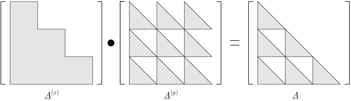
In [5] we prove a more general result so we will not give the details behind (12) here. Briefly, the first step is to observe that AA is the element-wise product (Hadamard product) of the two matrices A(x)A^{(x)} and A(y)A^{(y)}, where

Ai,j(x)=(L⁡(i)L⁡(j)),Ai,j(y)=(M⁡(i)M⁡(j)),A^{(x)}_{i,j}=\binom{L(i)}{L(j)}\,,\quad A^{(y)}_{i,j}=\binom{M(i)}{M(j)}\,,

and A(x)A^{(x)} is, as a whole, block lower-triangular with k×kk\times k size blocks while in A(y)A^{(y)} the separate k×kk\times k blocks are each lower triangular. See Figure 3. It follows that AA is lower-triangular.

Refer to caption
Figure 3. Shapes of A(x)A^{(x)}, A(y)A^{(y)} and AA. The matrix AA on the right is the Hadamard product of the matrices on the left.

The diagonal elements of AA are all 11 so detA=1\det A=1. Defining B=(−1)L⁡(i)+L⁡(j)+M⁡(i)+M⁡(j)​Ai,jB=(-1)^{L(i)+L(j)+M(i)+M(j)}A_{i,j} one then shows directly that B​ABA is the identity matrix, and this requires some special identities for binomial coefficients.

From the formula for A−1A^{-1} let us derive (11). We have

β¯=A−1ξ¯,b(k)l,m=βi,where i=k⁡(l−1)+m,\underline{\beta}=A^{-1}\underline{\xi}\,,\quad b^{(k)}_{l,m}=\beta_{i}\,,\quad\text{where $i=k(l-1)+m$,}

or

bl,m(k)\displaystyle b^{(k)}_{l,m} =βi=∑j=1k2Ai,j−1​ξj=∑j=1k2Ai,j−1​(L⁡(j)​M​(j)k)\displaystyle=\beta_{i}=\sum_{j=1}^{k^{2}}A_{i,j}^{-1}\xi_{j}=\sum_{j=1}^{k^{2}}A_{i,j}^{-1}\binom{L(j)M(j)}{k}
=∑j=1k2(−1)L⁡(i)+L⁡(j)+M⁡(i)+M⁡(j)​Ai,j​(L⁡(j)​M​(j)k)\displaystyle=\sum_{j=1}^{k^{2}}(-1)^{L(i)+L(j)+M(i)+M(j)}A_{i,j}\binom{L(j)M(j)}{k}
=∑j=1k2(−1)L⁡(i)+L⁡(j)+M⁡(i)+M⁡(j)​(L⁡(i)L⁡(j))​(M⁡(i)M⁡(j))​(L⁡(j)​M​(j)k).\displaystyle=\sum_{j=1}^{k^{2}}(-1)^{L(i)+L(j)+M(i)+M(j)}\binom{L(i)}{L(j)}\binom{M(i)}{M(j)}\binom{L(j)M(j)}{k}\,.

For L⁡(i)L(i) and M⁡(i)M(i), using 1≤m≤k1\leq m\leq k it is easy to verify that

L⁡(i)\displaystyle L(i) =⌊i−1k⌋+1=⌊k⁡(l−1)+m−1k⌋+1=l\displaystyle=\left\lfloor\frac{i-1}{k}\right\rfloor+1=\left\lfloor\frac{k(l-1)+m-1}{k}\right\rfloor+1=l
M⁡(i)\displaystyle M(i) =((i−1)modk)+1=((k⁡(l−1)+m−1)modk)+1=m.\displaystyle=((i-1)\mod k)+1=((k(l-1)+m-1)\mod k)+1=m.

To simplify the L⁡(j)L(j) and M⁡(j)M(j) terms, express jj as the combination

j=k​s+t,s∈{0,1,…,k−1},t∈{1,2,…,k}.j=ks+t,\qquad s\in\{0,1,\ldots,k-1\},\quad t\in\{1,2,\ldots,k\}\,.

Then just as above,

L⁡(j)\displaystyle L(j) =L⁡(k​s+t)=⌊k​s+t−1k⌋+1=⌊s+t−1k⌋+1=s+1\displaystyle=L(ks+t)=\left\lfloor\frac{ks+t-1}{k}\right\rfloor+1=\left\lfloor s+\frac{t-1}{k}\right\rfloor+1=s+1
M⁡(j)\displaystyle M(j) =M⁡(k​s+t)=((k​s+t−1)modk)+1=(t−1)modk+1=t−1+1=t.\displaystyle=M(ks+t)=((ks+t-1)\mod k)+1=(t-1)\mod k+1=t-1+1=t.

Hence,

bl,m\displaystyle b_{l,m} =∑j=1k2(−1)L⁡(i)+L⁡(j)+M⁡(i)+M⁡(j)​(L⁡(i)L⁡(j))​(M⁡(i)M⁡(j))​(L⁡(j)​M​(j)k)\displaystyle=\sum_{j=1}^{k^{2}}(-1)^{L(i)+L(j)+M(i)+M(j)}{{L(i)}\choose{L(j)}}{{M(i)}\choose{M(j)}}{{L(j)M(j)}\choose k}
=∑s=0k−1∑t=1k(−1)L⁡(i)+L⁡(k​s+t)+M⁡(i)+M⁡(k​s+t)​(L⁡(i)L⁡(k​s+t))​(M⁡(i)M⁡(k​s+t))​(L⁡(j)​M​(k​s+t)k)\displaystyle=\sum_{s=0}^{k-1}\sum_{t=1}^{k}(-1)^{L(i)+L(ks+t)+M(i)+M(ks+t)}{{L(i)}\choose{L(ks+t)}}{{M(i)}\choose{M(ks+t)}}{{L(j)M(ks+t)}\choose k}
=∑s=0k−1∑t=1k(−1)l+s+1+m+t​(ls+1)​(mt)​((s+1)​tk)\displaystyle=\sum_{s=0}^{k-1}\sum_{t=1}^{k}(-1)^{l+s+1+m+t}{{l}\choose{s+1}}{{m}\choose{t}}{{(s+1)t}\choose k}
=∑s=1k∑t=1k(−1)l+s+m+t​(ls)​(mt)​(s​tk),\displaystyle=\sum_{s=1}^{k}\sum_{t=1}^{k}(-1)^{l+s+m+t}{{l}\choose{s}}{{m}\choose{t}}{{st}\choose k}\,,

which is (11).

We conclude this part of the discussion by noting that we have three different expressions for the cc’s (or the bb’s), (7), (8) and (11) – and we do not know algebraically how to derive one from another!

5. More than two Variables

For an expansion

(x1x2⋯xn)k¯=∑LcL(k)x1l1¯x2l2¯⋯xnln¯,L=(l1,l2,…,ln),1≤li≤k,{(x_{1}x_{2}\cdots x_{n})}^{\underline{k}}=\sum_{L}c^{(k)}_{L}{{x_{1}}}^{\underline{{l_{1}}}}{{x_{2}}}^{\underline{{l_{2}}}}\cdots{{x_{n}}}^{\underline{{l_{n}}}}\,,\quad L=(l_{1},l_{2},\dots,l_{n})\,,1\leq l_{i}\leq k\,,

of a product of more than two variables all the results in the preceding sections have natural extensions. Modifications to the earlier arguments are straightforward and so we record the outcomes with little additional detail – the chief problem is notation. We follow the generally accepted conventions on multi-indexing. In particular

L!=l1!l2!⋯ln!.L!=l_{1}!l_{2}!\cdots l_{n}!\,.

The formula for the cc’s in terms of Stirling numbers is

cL(k)=∑p=1k(−1)k−p​[kp]​∏i=1n{pli}.c^{(k)}_{L}=\sum_{p=1}^{k}(-1)^{k-p}\left[\begin{matrix}{k}\\ {p}\end{matrix}\right]\prod_{i=1}^{n}\left\{\begin{matrix}{p}\\ {l_{i}}\end{matrix}\right\}\,.

or simply

cL(k)=∑p=1k(−1)k−p​[kp]​{pL}.c^{(k)}_{L}=\sum_{p=1}^{k}(-1)^{k-p}\left[\begin{matrix}{k}\\ {p}\end{matrix}\right]\left\{\begin{matrix}{p}\\ {L}\end{matrix}\right\}\,.

if we allow ourselves the analog to the the multi-indexed case of binomial coefficients and write

{pL}=∏i=1n{pli}.\left\{\begin{matrix}{p}\\ {L}\end{matrix}\right\}=\prod_{i=1}^{n}\left\{\begin{matrix}{p}\\ {l_{i}}\end{matrix}\right\}\,.

There is a natural extension of the product rule for the forward difference operator and it can be applied just as before to obtain a recurrence relation. It will pay to invest in a little extra notation. We write

L+1=(li+1:i=1,…,n)L+1=(l_{i}+1\colon i=1,\dots,n)

and for a subset S⊆{1,…,n}S\subseteq\{1,\dots,n\} we write

LS=(li:i∈S),LS+1=(li+1:i∈S),LS¯=(li:i∈{1,…,n}∖S).L_{S}=(l_{i}\colon i\in S)\,,\quad L_{S}+1=(l_{i}+1\colon i\in S)\,,\quad L_{\overline{S}}=(l_{i}\colon i\in\{1,\dots,n\}\setminus S)\,.

The result is

cL+1(k+1)=cL(k)−k​cL+1(k)+∑m=1n∑|S|=m(∏i∈Sli)​cLS+1,LS¯(k).c^{(k+1)}_{L+1}=c^{(k)}_{L}-kc^{(k)}_{L+1}+\sum_{m=1}^{n}\sum_{|S|=m}(\prod_{i\in S}l_{i})c^{(k)}_{L_{S}+1,L_{\overline{S}}}\,.

The generalization of a 2-dimensional conjoint ranking table allows for nn independent attributes (color, price, shape, …) with lil_{i} choices for the ii’th attribute. Based on the recurrence one can then show that L!​cL(k)L!c^{(k)}_{L} is the number of ways to fill in an l1×l2×⋯×lnl_{1}\times l_{2}\times\cdots\times l_{n} conjoint ranking table with the numbers 11 through kk, insisting, as before, that each attribute must enter into the ranking at least once. Again this implies the nonnegativity of the cc’s, more precisely

cL(k)=0c^{(k)}_{L}=0 if ∏ili<k\prod_{i}l_{i}<k and cL(k)>0c^{(k)}_{L}>0 if ∏ili≥k\prod_{i}l_{i}\geq k.

Extensions of the alternate formulas (8) and (11) are more complicated to write. For the former, to keep the final result from being too cluttered we use the notation

‖L‖=∑li∈Lli\|L\|=\sum_{l_{i}\in L}l_{i}

and for a multi-index M=(m1,m2,…,mn)M=(m_{1},m_{2},\dots,m_{n}) with 1≤mi≤h1\leq m_{i}\leq h and ‖M‖=h\|M\|=h we let

Φ⁡(L,M)=∏i=1nli−∑r=1n(lr​∏s<r(ls−ms)​∏s>rls)\Phi(L,M)=\prod_{i=1}^{n}l_{i}-\sum_{r=1}^{n}\left(l_{r}\prod_{s<r}(l_{s}-m_{s})\prod_{s>r}l_{s}\right)

Then

cL(k)=k!L!​∑h=0‖L‖(−1)h​∑M,‖M‖=h(Φ⁡(L,M)k)​∏j=1n(ljmj).c^{(k)}_{L}=\frac{k!}{L!}\sum_{h=0}^{\|L\|}(-1)^{h}\sum_{M,\|M\|=h}\binom{\Phi(L,M)}{k}\prod_{j=1}^{n}\binom{l_{j}}{m_{j}}\,.

While the derivation of this formula is only an extension of the argument for two variables, some discussion will help make the form clearer. Let “slices” refer to the higher-dimensional generalization of the notion of rows (or columns) for matrices. As before, we use inclusion-exclusion to count bL(k)b^{(k)}_{L}, the number of distinct l1×…×lnl_{1}\times\ldots\times l_{n} (0,1)(0,1)-tables with exactly kk ones and no zeroed slices; that’s the formula without the factorials in front. In the outer summation, the index hh is the number of zeroed slices. The inner summation then runs over possible ways to distribute the hh zeroed slices across the nn different dimensions. mim_{i} is the number of zeroed slices in dimension ii and (limi)\binom{l_{i}}{m_{i}} is the number of ways to select a particular set of mim_{i} slices to zero out. After counting ways to zero the slices, we must then count the number of ways to fill the remaining cells in the table with kk ones. The total number of cells in the array is ∏i=1nli\prod_{i=1}^{n}l_{i} and Φ⁡(L,M)\Phi(L,M) counts the remaining cells by subtracting the number of zeroed slices from the total number of cells. Then (Φ⁡(L,M)k)\binom{\Phi(L,M)}{k} is the number of ways to distribute kk ones among these remaining cells.

The analog of the formula (11) based on matrix inversion is developed in [5]. It reads

cL(k)=k!L!​∑r1,r2,…,rn=1k(−1)∑i(ri+li)​(∏irik)​∏i(liri).c^{(k)}_{L}=\frac{k!}{L!}\sum_{r_{1},r_{2},\dots,r_{n}=1}^{k}(-1)^{\sum_{i}(r_{i}+l_{i})}\binom{\prod_{i}r_{i}}{k}\prod_{i}\binom{l_{i}}{r_{i}}\,.

References

  • [1] Peter J. Cameron, Thomas Prellberg, and Dudley Stark, Asymptotics for incidence matrix classes, Electr. J. Comb. 13(1) (2006).
  • [2] Ch. A. Charalambides, Enumerative Combinatorics, Chapman & Hall/CRC Press, Boca Raton, 2002.
  • [3] R. Graham, D. Knuth, and O. Pasternik, Concrete Mathematics, 2nd ed., Addison Wesley, Reading, Massachusetts, 1994.
  • [4] M. Maia and M. Mendez, On the arithmetic product of combinatorial species, arXiv Math. (2008).
  • [5] Brad Osgood and William Wu, Inverses of generalized Pascal matrices, (to appear).
  • [6] R.P. Stanley, Log-Concave and Unimodal Sequences in Algebra, Combinatorics, and Geometry a, Annals of the New York Academy of Sciences 576 (1989), no. 1 Graph Theory and Its Applications East and West: Proceedings of the First China-USA International Graph Theory Conference, 500–535.