Inferring sparse Gaussian graphical models with latent structure
Abstract
Our concern is selecting the concentration matrix’s nonzero coefficients for a sparse Gaussian graphical model in a high-dimensional setting. This corresponds to estimating the graph of conditional dependencies between the variables. We describe a novel framework taking into account a latent structure on the concentration matrix. This latent structure is used to drive a penalty matrix and thus to recover a graphical model with a constrained topology. Our method uses an penalized likelihood criterion. Inference of the graph of conditional dependencies between the variates and of the hidden variables is performed simultaneously in an iterative em-like algorithm. The performances of our method is illustrated on synthetic as well as real data, the latter concerning breast cancer.
keywords
[class=AMS] Primary 62H20 , 62J07 ; secondary 62H30keywords
Gaussian graphical model , Mixture model , -penalization , Model selection , Variational inference , EM algorithm, and
Laboratoire Statistique et Génome
523, place des Terrasses de l’Agora
91000 Évry, FRANCE
??; ??; ??
??
Contents
1 Introduction
Estimating the concentration matrix (namely the inverse of the covariance matrix) of a Gaussian vector in a sparse, high-dimensional setting has received much attention recently. Graphical models provide a convenient setting for modelling multivariate dependence patterns. In this framework, an undirected graph is matched to the Gaussian random vector, where each vertex corresponds to one coordinate of the vector, and an edge is not present between two vertices if the corresponding random variables are independent, conditional on the remaining variables. Now, conditional independence between two coordinates of the Gaussian random vector corresponds exactly to a zero entry in the concentration matrix. Thus, detecting nonzero elements in the concentration matrix is equivalent to reconstructing the Gaussian graphical model (Lauritzen 1996, GGM, see e.g.).
We focus here on the crucial problem of selecting the concentration
matrix’s nonzero coefficients. In other words, we focus on variable
selection rather than estimation. Application areas include
gene-regulation graph inference in Biology (using gene expression
microarray data), as well as spectroscopy, climate studies, functional
magnetic resonance imaging, etc. We provide a very novel approach
driving the graph selection according to an unobserved modular
structure on the vertices.
The idea of covariance selection first appeared in the work of Dempster (1972). In the so-called “large , small ” setting (namely when the number of observations is smaller than the dimension of the observed response), the need for covariance selection is huge, as the empirical covariance matrix is no longer regular.
In Drton and Perlman (2007), a classification of the different methods for model selection/estimation in GGMs into three group types is suggested: constraint-based methods, performing statistical tests; Bayesian approaches; and score-based methods, maximizing a model-based criterion. The multiple testing problem has been taken into account in Drton and Perlman (2007), Drton and Perlman (2008). The authors perform GGM covariance selection by multiple testing of hypotheses about vanishing partial correlation coefficients. Such procedures may also be implemented using the PC-algorithm (Kalisch and Bühlmann 2007). Starting from a complete, undirected graph, the PC-algorithm deletes edges recursively, according to conditional independence decisions. However, the statistical procedure in Drton and Perlman (2007) relies on asymptotic considerations, a regime never attained in real situations.
Another attempt in this vein is to consider limited-order partial
correlations (Wille and Bühlmann 2006, Castelo and Roverato 2006). In
Wille and Bühlmann (2006) the authors consider only zero and
first-order conditional dependencies. They argue that for sparse
graphical models, these low-order dependencies still reflect
reasonably well the full-order conditional dependency structure.
Moreover, these dependencies may be well estimated even with a small
number of observations. In Castelo and Roverato (2006), the authors
introduce a non-rejection rate to reduce the multiple testing
and computational problems to which these approaches give rise.
A Bayesian framework is proposed in
Dobra et al. (2004), Jones et al. (2005) and their method was applied for
evaluating patterns of association in large-scale gene expression
data. The approach is based on dependency networks, namely a
collection of conditional distributions
(where
stands for the set of all variables but ). However, such
conditional distributions will not in general result in a coherent
joint distribution. This point is further discussed below concerning
a similar problem appearing in Meinshausen and Bühlmann (2006). Moreover,
constructing priors on the set of concentration matrices is not a
trivial task (it mainly relies on Wishart priors). The use of MCMC
procedures limits the range of applications to moderate-sized networks.
Before focusing on score-based methods, let us first introduce regularization procedures. In the context of linear regression, the Lasso (least absolute shrinkage and selection operator) technique was introduced by Tibshirani (1996). This procedure performs model selection and parameter estimation at the same time. The idea is that ordinary least-squares criterion may be improved in a sparse context, using an -norm penalty. The -norm penalty shrinks the estimates to zero while preserving the convexity of the optimization problem. Note that the -norm penalization is also known as ’basis pursuit’ in signal processing (Chen et al. 2001).
It is well known that if the ultimate goal is parameter estimation, model selection and estimation should be done in a single step. Performing the model selection prior to parameter estimation in the selected model will, in fact, result in a non-robust procedure. However, our primary focus here is on model selection, as we want to infer sparse networks. We therefore concentrate on model selection rather than on estimation performances.
The Lars algorithm (Efron et al. 2004) is one of the most popular techniques for solving the Lasso problem. It gives the path of solutions obtained when varying the penalty parameter (the penalty parameter is used as a scaling factor of the -norm penalty). The larger the penalty parameter, the sparser the Lasso solution.
Using convex optimization techniques (Minoux 1986, see for
instance), the Lasso problem may be
stated as a primal problem, whose dual formulation may be solved more
easily. This approach is taken in Osborne et al. (2000b). The
authors obtain an iterative algorithm, the “homotopy method”
(Osborne et al. 2000a). Other very efficient approaches are based on
focusing on each coordinate iteratively. Indeed, for each coordinate,
the Lasso problem is solved very simply (assuming the other
coordinates are fixed) by soft-thresholding (Donoho and Johnstone 1995).
Thus, different ’coordinate optimization’ procedures have been
proposed in the literature. Following the work of
Fu (1998), a cyclic procedure is proposed in
Friedman et al. (2007), where optimization with respect to each
coordinate is done iteratively; whereas Wu and Lange (2008) propose a
greedy approach, computing the solution for each coordinate and
choosing that which provides the largest decrease in a surrogate objective
function. Note that these approaches rely on the underlying assumption
that the predictors for the regression problem are uncorrelated.
Let us now come back to covariance (or concentration) matrix inference in GGMs, using maximization of a model-based criterion.
Meinshausen and Bühlmann (2006) were the first authors to apply Lasso techniques for inferring a covariance matrix in a GGM. Their approach is to solve different Lasso regression problems, where is the dimension of the observed vector. The main drawback of such a procedure is that a symmetrization step is required to obtain the final network. It might, for instance, be the case that the estimator of the regression coefficient for on is zero, whereas the estimator for on is not zero. Meinshausen and Bühlmann propose to use either an “AND” or an “OR” final step procedure to recover an undirected correlation graph. However, these two procedures might result in different estimates and there is no way of choosing between them. Moreover, as previously stated, a set of conditional distributions does not necessarily cohere into a joint distribution. Using a set of possibly non-coherent conditional distributions corresponds to a pseudo-likelihood approach. This aspect was not underlined in Meinshausen and Bühlmann (2006), and we clarify this point in Section 4.
Subsequently, two other articles, Banerjee et al. (2008) and Yuan and Lin (2007) independently provided an improvement of the initial work of Meinshausen and Bühlmann (2006). In both works, the problem is seen as a penalized maximum-likelihood (PML) problem. Instead of considering different regression problems, these two articles focus on the likelihood of the Gaussian vector, penalizing the entries of the concentration matrix with an -norm penalty. They explain how the PML estimation may be solved as a “Lasso-like” problem. The major issue with PML strategies in the context of the concentration matrix estimation of GGMs is to obtain a positive definite estimate. However, the approach for solving the problem in Yuan and Lin (2007) is not suited to high-dimensional settings, in contrast to the approach proposed in Banerjee et al. (2008). In Yuan and Lin (2007), a non-negative garrote-type estimator is used, and asymptotic properties (as tends to infinity while is held fixed) are given. In Banerjee et al. (2008), two different algorithms are proposed for solving problems in a high-dimensional setting. The first approach relies on a block-coordinate descent algorithm. The second is a semi-definite programming algorithm, based on Nesterov’s method, which is computationally intensive.
The next improvement in this vein comes with Friedman et al. (2008). Relying on coordinate descent techniques, previously described in Friedman et al. (2007), the authors revisit Banerjee et al.’s first approach and propose an efficient algorithm to solve the PML estimation problem, under the positive definite constraint. In fact, they use the block coordinate descent approach proposed by Banerjee et al. (2008) and combine it with a second coordinate descent method. Our method will make use of this approach.
To conclude this part, we remark that a completely different shrinkage
estimate was proposed by Schäfer and Strimmer (2005) in the same
context of large-scale covariance matrix estimation. The approach
consists in using a weighted average of two different estimators, the
first being unconstrained (thus having small bias but large variance),
the second being low-dimensional (and thus exhibiting small variance
but large bias).
Now let us motivate the use of hidden structures in networks.
Modularity is a property observed in real (biological) networks
(Ihmels et al. 2002, see for instance). Heterogeneity in
the node behaviors is an important property of these data. For
example, so-called ’hubs’ are highly-connected nodes, showing a
different behavior from the rest of the graph nodes. An interesting
model capturing these network features is a mixture model for random
graphs (Daudin et al. 2008, see for instance). This model has been
rediscovered many times in the literature, and a non-exhaustive
bibliography should include Frank and Harary (1982), Snijders and Nowicki (1997), Nowicki and Snijders (2001), Tallberg (2005), Daudin et al. (2008), Mariadassou and Robin (2007), Zanghi et al. (2008). To
state it simply, this model assumes that each
node belongs to some unobserved group. Conditional on the node groups,
the (weighted) edges are independent and identically-distributed
(i.i.d.) random variables, whose distribution depends on the groups
of the nodes to be connected. As we are interested in GGMs, weighted
edges correspond to entries of the concentration matrix.
In this work, we aim at estimating a hidden structure, namely node
groups, while discovering the network. This hidden structure should
help us in choosing adaptive penalty parameters. Indeed, we
wish to penalize the elements of the concentration matrix, according
to the unobserved clusters to which the nodes belong. For instance, if two nodes
belong to the same unobserved group, we wish to lower the penalty
parameter acting on the corresponding entry in the concentration
matrix. Conversely, if we increase the penalty parameters on the
entries corresponding to nodes belonging to different groups, we
shrink the estimated coefficient to zero. Our approach is completely
new and improves inference of sparse modular networks.
Another adaptive Lasso procedure is given in Zou (2006), whose idea is to lower the bias of the large coefficients by adapting the penalty parameter of each coefficient so that it automatically scales with the inferred value. It is known that the non-adaptive Lasso procedure may result in inconsistent parameter estimation. An illustration of the conflict between optimal prediction and consistent variable selection for the Lasso procedure is given in Meinshausen and Bühlmann (2006). They proved that the optimal penalty parameter for prediction gives inconsistent variable selection results, motivating the use of another penalty parameter to ensure the control of the probability of falsely connecting two or more distinct connectivity components of the graph. Like them, we also focus on optimal selection rather than on optimal prediction. The adaptivity of our procedure is not used for lowering the bias of large coefficients, but instead for constraining the prediction to fit the underlying structure of the graph.
Model.
Let us now briefly describe the general approach of our work. The model will be presented in detail in Section 2. Let be a Gaussian random vector in , with zero mean and positive definite covariance matrix , namely We observe independent and identically-distributed (i.i.d) vectors with the same distribution as . The matrix is the concentration matrix of the model. Let be the empirical covariance matrix. The log-likelihood of the observations is given by
where is a constant term.
The -penalized estimator proposed by Banerjee et al. (2008) is given by
| (1) |
where stands for positive definiteness, is a penalty parameter and .
A natural generalization of this approach is to have different penalty parameters for different entries . Namely,
where is a matrix of penalty functions acting on each entry. As a general rule, using as many penalty functions as there are entries in the concentration matrix to be estimated is not meaningful.
Here, we propose to take into account a hidden structure on the correlations between the coordinates random variables . Thus, we consider latent i.i.d. random variables with values in a finite set . Each variable describes the state of , and we wish to adapt the penalty function with respect to the states of . More precisely, we wish to use a criterion of the form
where is a matrix of random penalty functions whose entries depend on the latent structure . However, the hidden structure is not supposed to be known, thus we cannot rely on the previous criteria. Intuitively, following the principle of Expectation-Maximization (em) algorithm of Dempster et al. (1977), the idea will be to replace the unobserved value with its conditional expectation under some model with parameter , and iterate the following steps
- (e)
Compute
- (m)
Update .
One of our aims is to provide a very simple framework for such an analysis.
Note that the -norm used here acts on diagonal elements of the matrix . It is counter-intuitive to penalize diagonal elements of the concentration matrix, as these do not reflect sparsity in the correlation structure. However, from a technical point of view, this strategy ensures that the procedure will select a positive definite estimator (see Remark 2). This point was not emphasized in the previous procedures using penalized likelihood of GGMs.
Road-map.
In Section 2 we present the model and the penalized
maximum-likelihood criterion on which we base our inference procedure,
described in Section 3. This procedure relies on
a variational em algorithm, combined with a Lasso-like
procedure. Section 4 explains how
Meinshausen and Bühlmann’s approach may be interpreted as a
penalized pseudo-likelihood method. Finally, Section 5
illustrates the performance of the method on synthetic data, for which
an R–package, SIMoNe (Statistical Inference for
Modular Network), can be downloaded from the first author’s website. We
also test our algorithm on a real data set provided by
Hess et al. (2006) and concerning patients with breast
cancer treated using chemotherapy. According to Hess et al. (2006)
and Natowicz et al. (2008), the patient response to the treatment can
be classified either as a pathologic complete response (pCR), or
as a residual disease (not-pCR). The prediction of the patient response is
achieved accurately by studying the expression levels of a limited
number of genes (). Our algorithm is applied on each class of
patients (pcR and not-pCR). Two distinct gene-regulatory networks are
thus inferred, showing a very different structure according to the
selected class of patients.
2 A latent structure model for network inference
In this section we present a framework for modelling heterogeneity among dependencies between the variables. To this end, let us first recall classical notations from Gaussian Graphical Models (see Lauritzen 1996, for elementary results about GGMs).
2.1 Gaussian graphical models: general settings
Let be a set of fixed vertices, a random vector describing a signal over this set and a sample of size with the same distribution as .
The vector is assumed to be Gaussian with positive definite covariance matrix . No loss of generality is involved when centering , so we may assume that . GGMs are based on a classical result, originally emphasized by Dempster (1972), claiming that any couple of entries with are independent conditional on all other variables indexed by , if and only if the entry is zero. The inverse of the covariance matrix , known as the concentration matrix, thus describes the conditional independence structure of . Moreover, each entry is directly linked to the partial correlation coefficient between variables and . In fact, we have , and also . Hence, after a simple rescaling, the matrix can be interpreted as the adjacency matrix of an undirected weighted graph representing the partial correlation structure between variables . This graph has no self-loop, with a random set of edges composed by all pairs such that . Note that we are seeking only pairs of vertices such that , since there is no self-loop, and since . Inferring nonzero entries of is equivalent to inferring , and is therefore a highly relevant issue in this framework.
2.2 Providing the network with a latent structure
Let us now extend the modeling by providing the network with an internal latent structure.
The model proposed in Daudin et al. (2008) attempts a better fit of data, as it places the network in the mixture framework, in order to take account of the heterogeneity among vertices. The same general mixture model is adopted here: vertices of are distributed among a set of hidden clusters that model the latent structure of the network. For any vertex , the indicator variable is equal to if and otherwise, hence describing which cluster the vertex belongs to. A vertex is assumed to belong to one cluster only, thus the random vector obviously follows a multinomial distribution. Namely,
| (2) |
where is a vector of cluster proportions, so that .
The concentration matrix structure.
We shall now extend the clustering of vertices from to the concentration matrix . Accordingly, both the existence and the weight of edges, described by the off-diagonal elements of , will depend on the cluster each vertex belongs to. Conditional on the events and where are clusters chosen from , each () is a random variable whose probability density function is denoted by , that is,
| (3) |
It will be remarked that in this formulation the variables are assumed to be independent, conditional on the clusters the vertices belong to. Moreover, we are considering only undirected graphs, so we may assume that . For technical reasons (see Remark 2), we also assume a prior distribution on diagonal elements of , namely
Our suggestion is to adopt Laplace distributions; hence
| (4) |
where are scaling parameters and . Below, the parameter will be fixed and not estimated.
The reason for choosing a Laplace distribution is that it is reminiscent of the -norm, itself linked to Lasso-techniques for which appropriate tools are available. In fact, when considering the general penalized least-square problem, the penalty term can be seen as a log-prior density on the vector of parameters. In the case of Lasso, the prior distribution corresponding to the -norm is actually the Laplace distribution (Hastie et al. 2001, see, e.g.).
The affiliation model.
The affiliation model is a special case of network structure (to be investigated below), where there are many different clusters, but where the focus is restricted to two types of edges: edges between nodes of the same cluster, and edges between nodes from different clusters. In the affiliation model the densities in (4) are of only two kinds; that is, for all , let
| (5) |
2.3 The complete likelihood
Having described the modeling of the network, we now focus on the inference issue.
We denote as the matrix that contains the data-set row-wisely organized, i.e., is the row of . Furthermore, we denote as the set of all latent indicator variables for vertices. For the sake of simplicity, the number of clusters and the parameters and are assumed to be known for the moment.
The data experiments are the only observations available, and from these we should like to be able to infer the graph of conditional dependencies or, equivalently, nonzero entries of . As the matrix has been given a prior distribution, our aim is to maximize the posterior probability of , given the data , or equivalently, the logarithm of the joint distribution. The estimate is thus defined as follows:
where stands for positive-definiteness.
To solve this problem, we place ourselves in the classical complete-data framework. The distribution of is only known conditionally on the latent structure described by . We denote as the set of all possible clusterings over nodes from . The marginalization over the latent clusters leads to
where the so-called complete-data likelihood is the function we shall develop using an em-like strategy hereafter. For this purpose, a closed form of is required.
Proposition 1.
The following relation holds for the complete-data likelihood .
| (6) |
where is the empirical covariance matrix, is a constant term and is defined by
| (7) |
Proof.
Using the Bayes rule, divides into three terms:
where we make use of the fact that .
3 Inference strategy by alternate optimization
In the classical em framework developed by Dempster et al. (1977), where is the available data, inferring the unknown parameters spread over a latent structure would make use of the following conditional expectation:
| (8) |
where is the estimation of from the
previous step of the algorithm.
The usual em strategy would be to alternate an E-step computing the conditional expectation (8) with an M-step maximizing this quantity over the parameter of interest . Unfortunately, no closed form of can be formulated in the present case. The technical difficulty lies in the complex dependency structure contained in the model. Indeed, cannot be factorized, as argued in Daudin et al. (2008). This makes the direct calculation of impossible. To tackle this problem we use a variational approach (see, e.g., Jaakkola 2000, for elementary results on variational methods). In this framework, the conditional distribution of the latent variables is approximated by a more convenient distribution denoted by , which is chosen carefully in order to be tractable. Hence, our em-like algorithm deals with the following approximation of the conditional expectation (8)
| (9) |
In the following section we develop a variational argument in order to choose an approximation of . This enables us to compute the conditional expectation (9) and proceed to the maximization step.
3.1 Variational estimation of the latent structure (E-step)
In this part, is assumed to be known, and we are looking for an approximate distribution of the latent variables. The variational approach consists in maximizing a lower bound of the log-likelihood , defined as follows:
| (10) |
where is the Küllback-Leibler divergence. This measures the difference between the probability distribution in the underlying model and its approximation . An intuitively straightforward choice for is a completely factorized distribution (Mariadassou and Robin 2007, Zanghi et al. 2008, see)
| (11) |
where is the density of the multinomial
probability distribution , and
is a random
vector containing the variational parameters to optimize. The complete
set of parameters is what we are seeking
to obtain via the variational inference. In the case in
hand the variational approach intuitively operates as follows: each
must be seen as an approximation of the probability that
vertex belongs to cluster , conditional on the data, that is,
estimates , under the
constraint . In the ideal case where
can be factorized as
and the parameters
are chosen as , the Küllback-Leibler
divergence is null and the bound reaches the log-likelihood.
The following proposition gives the form of the lower bound to be maximized in order to estimate .
Proposition 2.
Proof.
Starting from (10), classical results on variational methods show that
where is the entropy of the distribution and is the approximation of the complete log-likelihood conditional expectation, computed under the distribution . Namely,
| (13) |
In the special case of factorized distribution (11), the entropy is
Moreover,
Equation (12) follows via Proposition 1, by using that and . ∎
The optimal approximate distribution is then derived by direct maximization of . The following proposition gives the estimate that solves the problem.
Proposition 3.
Let and be known. The following fixed-point relationship holds for the optimal variational parameters
| (14) |
where means that there is a scaling factor such that for any , we have .
Proof.
This is just an adaptation to the Laplace case of Mariadassou and Robin (2007, Proposition 3). ∎
The initial value of is chosen using a classification algorithm such as spectral clustering (Ng et al. 2002, see for instance). As a consequence, the initial values for lie in . We then use an iterative procedure setting , where is the function (implicitly defined above) for which is a fixed point. Note that we cannot ensure uniqueness of the fixed point for , nor convergence of this iterative procedure. In practice, we can always use a maximal number of iterations, and if convergence has not occurred, we keep the initial value of given by the clustering method. In appendix A.2 we explain that at least in the affiliation model (5), if the current values of the precision matrix are small enough, and if the penalty parameters and are well-chosen, then uniqueness of the fixed point is ensured. However, such a result does not hold in the general case, which is one of the drawbacks of of the variational approach in this context.
Estimation of and .
The parameters and have been previously considered as known to keep the statement as clear as possible.
Two different strategies may be used with respect to these parameters. The first approach is to fix their values. Fixing the value of comes down to choosing a priori the proportions of the groups, which is quite a common strategy in mixture models. As for the choice of , this is equivalent to choosing the penalty parameter in the classical lasso. Concerning general parameters , a number of values need to be determined, which might be a problem. However in the particular affiliation model (5), only parameters have to be fixed: a parameter that corresponds to a light penalty, since many intra-cluster edges are expected, and another parameter that fits with a heavier penalty, since we do not expect many inter-cluster edges. This is typically the kind of strategy that will be used for numerical applications (see Section 5). More generally, the matrix penalty can be tuned to obtain a desired quantity of inferred edges, or to constrain the topology of the graph, e.g. graphs with hubs.
The second strategy is to make use of the current inferred graph to estimate the parameters. The basic idea is to include this estimation in the variational method. Unfortunately, the maximization of given in equation (12) with respect to , and at the same time is not possible. To tackle this problem, we use an alternate strategy. The parameter is computed with the fixed-point relationship (14) for fixed values of and . Then we maximize with respect to and , once is fixed (that is, once is fixed), as in the following proposition. We successively iterate these two steps until stabilization.
Proposition 4.
For fixed values of , the parameters , maximizing are given by
Proof.
Once terms that do not depend on the parameters of interest have been removed from , the problem becomes
Null-differentiation with respect to (under the constraint ) and leads straightforwardly to the result. ∎
3.2 A Lasso-like method to estimate the concentration matrix (the M-step)
Now that we are able to compute the approximate conditional expectation defined by (13), we wish to infer the concentration matrix , assuming is known. This is the aim of the m-step of our em–like strategy, that deals with the maximization problem .
Using Proposition 1 and the equality , it is a simple matter to rewrite the problem as follows
| (15) |
Hence, our m–step can be seen as a penalized maximum likelihood estimation problem, exactly like in Friedman et al. (2008), Banerjee et al. (2008). The likelihood considered here is , that is, the likelihood which corresponds to the realizations of the Gaussian vector for a given concentration matrix . The difference of our approach lies in the complexity of the penalty term, and in slight discrepancies as regards some constant factors.
Remark 1.
Since we are using a penalty term on matrix ’s diagonal elements, the solution to (15) satisfies
| (16) |
when for any . Indeed, the sub-gradient equation is , and since it is the inverse of a conditional variance.
Let us now look at the solution of the m-step: the following proposition gives an equivalent formulation of (15) that is more likely to be solved. The result draws its inspiration from Banerjee et al. (2008).
Proposition 5.
The maximization problem (15) over the concentration matrix is equivalent to the following, dealing with the covariance matrix
| (17) |
where is the term-by-term division and
Remark 2.
By penalizing the diagonal terms of the concentration matrix in the initial problem, the set of matrices over which we maximize our criterion contains, for instance, the matrix , (where stands for the identity matrix). Thus, provided that the value of penalty parameter is set sufficiently high, this set contains positive definite matrices. This ensures that our estimator is always invertible. Obviously, when is invertible, which is usually true for greater or equal than , penalizing the diagonal terms becomes futile. In this case is set to zero.
Proof.
The penalty term in (15) can be written as follows
where is the term-by-term product. The set contains symmetric matrices, defined, for each couple , by
Let us now use the fact that , for a given matrix . The optimization problem (15) can now be written as
since the trace operator is linear. The dual version of the above expression is obtained by swapping and . The maximization is solved by differentiating with respect to . To do this, we recall that in our specific case the matrices are symmetrical, and thus . Then, applying the usual rules for the derivative of the trace operator, null-differentiation with respect to yields
| (18) |
The dual problem therefore becomes
or in other words,
Finally, we need to write the constraint as a function of rather than the set . In fact, we simply need to show that
which is straightforward (see Appendix A.1 for details). ∎
To solve (17) and thus obtain the estimate
, we successively use two coordinate
descent methods. The first corresponds to a block-wise strategy
suggested by Banerjee et al.. The second one is used
to solve the resulting Lasso problem and was suggested by
Friedman et al. (2007).
Let us first explain the block-wise strategy. For this purpose, we introduce the following notation for , and the penalty matrix
| (19) |
where , and are matrices, , and are length column vectors and , and are real numbers. We have already remarked (Remark 1) that the solution to (17) satisfies . Moreover, using Schür complement, the vector satisfies
| (20) |
We have . The full matrix is approximated in the following way: first, if required when is greater than , we initialize the procedure with , where is chosen so as to make invertible; secondly, we permute the columns (and thus the rows) of and iteratively solve problems like (20) until convergence of the procedure. This convergence is ensured by the following lemma.
Lemma 1.
Proof.
The proof relies on Banerjee et al. (2008, Theorem 3) and Tseng (2001, Theorem 4.1). Convergence of block-coordinate descent methods is a well-documented topic in convex optimization literature. Here, we have to bear in mind that using -norm penalty leads to non-differentiable functions. Thus, we rely on a result by Tseng (2001, Theorem 4.1), which in our case ensures the convergence of the procedure, provided there is at most one solution to each minimization problem (20). This point is proved in Banerjee et al. (2008, Theorem 3). ∎
Then, starting from a result given in Banerjee et al. (2008), an interpretation of (20) as an –penalized problem is given in Friedman et al. (2008). This –penalized problem is reminiscent of the Lasso and may thus be solved using a coordinate descent strategy (Friedman et al. 2007). The following proposition enunciates a result similar to those obtained in Banerjee et al. (2008, equation (6)) and Friedman et al. (2008, equation (2.4)), although with a more general penalty term and a factor that differs. Since none of these articles gives an explicit proof for this result, it is fitting that we provide our own proof here.
Proposition 6.
Proof.
Problem (20) can be written as follows, by splitting the constraint:
Let us introduce the so-called Lagrangian, with vectors of Lagrange coefficients denoted by with nonnegative entries. Also, let . The Lagrange version of the above problem is
| (23) |
where, in the present case, is given by
The coefficients and maximizing are null when the constraints are satisfied, and for each index , at least one coefficient among is zero. Then
Meanwhile, consider the dual problem of (23), swapping and : the solution that minimizes the dual problem with respect to satisfies the null-gradient hypothesis. We obtain , that is (which proves equation (22)). Introducing this result in the dual of (23), we get
also equivalent to
Expressing this quantity by using the Euclidean norm achieves the proof. ∎
Hence, the column of the estimated covariance matrix is computed by solving the Lasso problem (21) using another coordinate descent method.
Lemma 2.
The solution to (21) is computed by updating the th coordinate of via
| (24) |
where is the soft-thresholding operator.
Proof.
The proof of this lemma is postponed to Appendix A.3. ∎
Finally, the estimate of the matrix of concentration is
recovered by inverting , which can be
done at low computational cost (see appendix A.4 for
details). Hence, we solve the initial maximization problem
(15) that defines the m-step of our algorithm.
Implementation of the full em algorithm is outlined in Algorithm 1.
3.3 Choice of penalty parameters
As previously stated, the penalty parameters may be estimated in the e-step of the algorithm (see subsection 3.1). However, this choice is not necessarily optimal for the estimation of , and other choices might in practice lead to a better solution. A good strategy is to keep the estimated value of in the e-step that leads to the estimation of , and to impose another value of during the m-step. In this part, we indicate a possible choice for the penalty parameters to use in the m-step, ensuring a small error on the connectivity components of the estimated graph.
Let us first introduce some notation. For any node , let denote the connectivity component of node in the true underlying conditional dependency graph, and the corresponding component resulting from the estimate of this graph structure. The following proposition is based on Meinshausen and Bühlmann (2006, Theorem 2) and Banerjee et al. (2008, Theorem 2).
Proposition 7.
Fix some and choose the penalty parameters such that, for all ,
| (25) |
where is the c.d.f. of Student’s -distribution with degrees of freedom. Then
| (26) |
Proof.
Here we simply indicate the main differences between the proof of Banerjee et al. (2008, Theorem 2) and what is valid in our context. Note that according to (15), the estimator must satisfy the following sub-gradient equation
where . Following the proof of Banerjee et al. (2008, Theorem 2), we easily get
Performing some computations involving the correlation between variables and , we also obtain
which entails the conclusion. ∎
Remark 3.
Following Banerjee et al. (2008), note that in order to ensure (25), it is enough to choose the penalty parameter such that, for all ,
where is the -quantile of Student’s -distribution with degrees of freedom, i.e. .
Remark 4.
Inequality (25) does not take into account that different penalty parameters are used for different hidden classes . An adaptation of the preceding strategy is to use current values obtained from the probabilities of the hidden classes and to choose the current penalty parameters accordingly. More precisely, let us set, for instance
Then, when
| (27) |
for all , the current estimate of the dependency graph will approximately satisfy (26). Moreover, in order to ensure (27), it is enough to choose, for all ,
| (28) |
4 Link with Meinshausen and Bühlmann’s approach
We should also like to fill the gap between, on the one hand solving (15) and, on the other, the approach proposed in Meinshausen and Bühlmann (2006), where independent penalized regression problems are solved using the Lasso. In fact, we shall show that Meinshausen and Bühlmann’s approach is equivalent to maximizing the penalized pseudo log-likelihood corresponding to the size- sample of the multivariate Gaussian vector on the set of non symmetric matrices. Let us denote as this pseudo-likelihood, defined by
where is the th realization of the Gaussian vector , once the th coordinate has been removed. In this section, the -norm of matrices is restricted to off-diagonal elements only, that is, .
Proposition 8.
Consider the solution to the penalized pseudo-likelihood problem
| (29) |
(whose diagonal is fixed) and the solution given in Meinshausen and Bühlmann (2006) to the different regression problems, using the matrix penalty . The two solutions have exactly the same null entries.
Proof.
Denote by and , respectively, the matrices and once their th row and th column have been removed. Moreover, and are the th rows of the matrices with the th term removed. After some routine computations, and using classical results for Gaussian multivariate vectors (see Appendix A.5), it can be shown that
| (30) |
where does not depend on . Thus, if we forget the symmetry constraint on , maximizing the pseudo-likelihood (30) with respect to the non-diagonal entries of is equivalent to independent maximization problems with respect to each column . Consider, for instance, the last column of , that is, for , and the relative term in (30). This term can be written as
where we use the block-wise notation defined above (19). The term does not depend on , which is the current column of the concentration matrix to infer. Namely, .
Consider now the penalized version of the log-likelihood (29): we wish to solve penalized problems of minimization as defined above, which can be written as follows
| (31) |
Meinshausen and Bühlmann wish to solve Lasso-problems, for instance for the last variable ,
| (32) |
where is the th column of and is the matrix of data the th column has been removed (note that we adapted the penalization term corresponding to the framework developed here).
The minimum is reached in (31) for null-differentiation, and we get
where . The same for (32), and we get
where . Now, just note that and , and problems (31) and (32) are equivalent, provided that .
Thus, the columns of the concentration matrix (with a removed diagonal term) inferred from the penalized maximum pseudo-likelihood problem (29), and those inferred with Meinshausen and Bühlmann’s approach, share exactly the same null-entries, that is, the same network of conditional dependencies. ∎
5 Numerical experiments
In this section we present numerical experiments on both synthetic data, to investigate how well the proposed selection procedure behaves, and real data, to demonstrate the practical use of GGM covariance selection with latent structure. In the remainder of this section we focus on an affiliation model (5), the choice of the penalty being made in line with Section 3.3. More precisely, we fix the ratio and either let the value vary when considering precision/recall curves for synthetic data, or fix this parameter according to (28) when dealing with real data.
5.1 Synthetic data
We perform numerical experiments to assess the performance of our approach (SIMoNe, Statistical Inference for Modular Network) and compare it to already existing methods for GGM covariance selection: GLasso (Friedman et al. 2008) and GeneNet (Schäfer and Strimmer 2005).
Data synthesis in our framework requires the simulation of a structured sparse inverse covariance matrix. To this aim, we first simulate a graph with an affiliation structure. We consider a simple binary affiliation model where two types of edges exist: edges between nodes of the same class and edges between nodes of different classes. The binary incidence matrix of the graph is transformed by randomly flipping the sign of some elements in order to simulate both positively and negatively correlated variables. Positive definiteness of this matrix is ensured by adding a large enough constant to the diagonal. The matrix is then further normalized to have a diagonal of ones. A Gaussian sample of size with zero mean and the above covariance matrix is then simulated 50 times. The results we present below are averaged over the 50 samples. At the end of this section we discuss the performances of our method when there is no latent structure on the data.
 |
 |
|
| (a) | (b) | (c) |
We simulate sparse graphs with and from 100 to 2000
(). We use
a probability of intra-cluster connection of , a probability
of inter-cluster connection of , groups and equal
group proportions . With these settings, the
theoretical expected number of edges is about 862 and the total number
of potential edges is 19900. A sample graph is given in
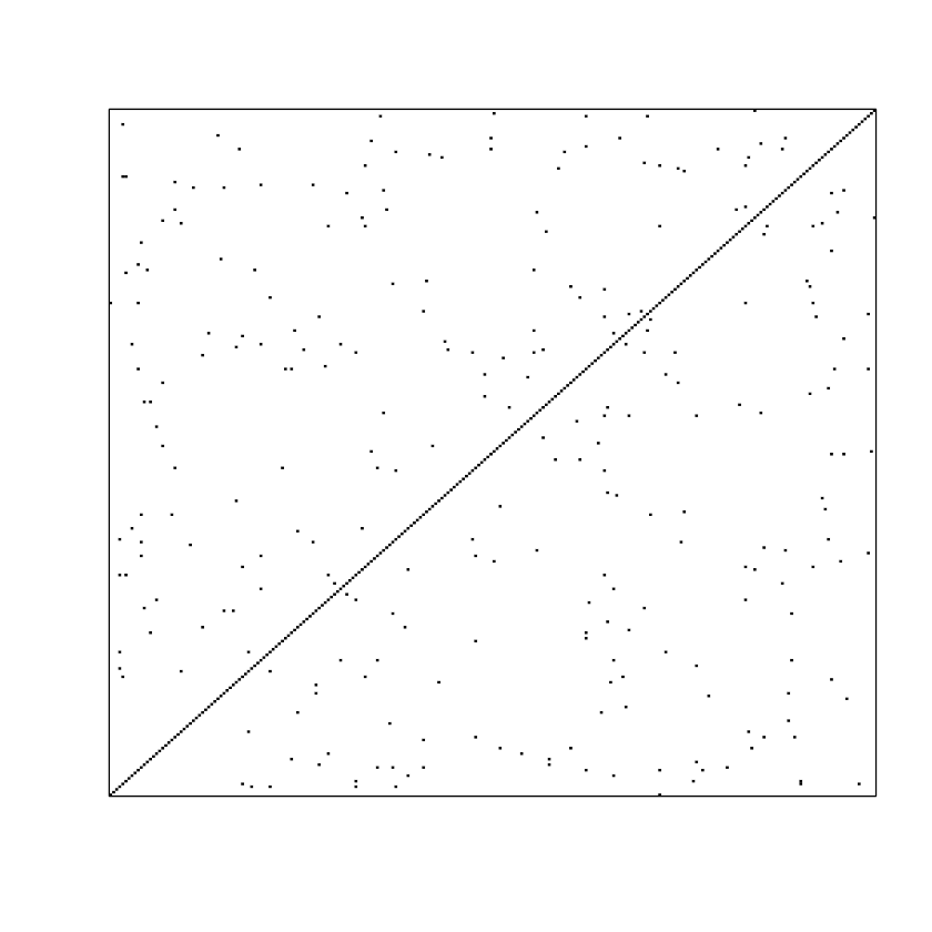
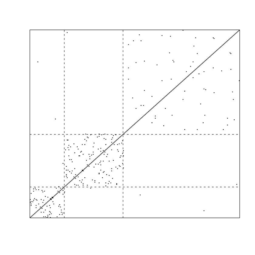
Figure 1. The running times of GLasso and SIMoNe are
of the same order. For the settings described above the running time
varies from a few seconds to a few minutes, according to the penalty parameter.
We focus the experiments on the ability to recover existing edges of the network, that is the nonzero entries of the concentration matrix. This is a binary decision problem where the compared algorithms are considered as classifiers. The decision made by a binary classifier can be summarized using four numbers: True Positives (), False Positive (), True Negatives () and False Negatives (). We have chosen to draw precision/recall curves to display this information and compare how well the methods perform (Figure 2).
Precision () is the ratio of the number of true nonzero elements to the total number of nonzero elements in the estimated concentration matrix . Recall that () is the ratio of true nonzero elements in to all nonzero entries of the real concentration matrix . In a sparse context where the number of actual positives () is small compared to the number of actual negatives (), precision/recall curves give a more informative picture of an algorithm’s performance than classical Receiver Operator Characteristic (ROC) curves. Indeed, ROC curves plot the False Positive Rate () against the True Positive Rate (). When the number of total positives is small compared to the number of total negatives, small variations of and will result in small variations of and large variations of , which is not relevant for comparing performances. In a statistical framework, the recall is equivalent to the power and the precision is equivalent to one minus the False Discovery Proportion.
Additionally to the GLasso (Friedman et al. 2008) and GeneNet (Schäfer and Strimmer 2005) we consider two other procedures:
- •
When is greater than , a straightforward way to obtain an estimate of the inverse covariance matrix is to invert the empirical covariance matrix. Although this approach is unlikely to perform well in a selection context (since it is designed for estimation purposes), it is worth comparing it to its competitors in order to assess the scale of improvement. We call this procedure InvCor.
- •
When the latent structure of the concentration matrix is known, our method can be applied without its E-step and produce a relevant selection of the nonzero entries of the concentration matrix. This approach represents the upper limit of our method, since it makes use of an usually unavailable source of information. This procedure is denoted perfect SIMoNe.
In some problems the latent structure of the graph is partially known and this information can be used in the E-step to improve the estimation of the latent structure. For example, when inferring gene regulation networks, a subset of identified genes may be known to belong to the same functional module.
The approach of Meinshausen and Bühlmann (2006) was also tested. The principle of this approach, and the performances obtained are close to those of GLasso, but it was always slightly outperformed. We have therefore decided, for the sake of brevity, to report only the four previously described procedures.
For the methods based on penalization (GLasso, SIMoNe and Perfect SIMoNe), the precision/recall curves are plotted by varying the penalty parameter (namely in our case). The penalty parameter varies from close to zero to a maximum value which forces all off-diagonal elements of to be null (see Appendix A.6). The GeneNet and InvCor methods are plotted by sorting the elements of according to their absolute values, and choosing different thresholds to find nonzero entries.
Even when is really greater than (Figures 2 (a-b)) Invcor is always dominated by the other methods from a selection point of view. This simple check shows that even in a favorable context with abundant data, penalization procedures improve the selection of nonzero entries of the concentration matrix, in comparison with methods based on estimation of these entries.
Although GeneNet and GLasso can provide different results on a given run, both methods perform similarly on average (50 runs for our experiment). The only parameter we change in this experimental setting is the ratio.
Perfect SIMoNe’s curves dominate all other curves for any ratio. This clearly shows that the knowledge of the structure provides a valuable information for selecting the nonzero entries of the concentration matrix. When the structure is hidden, the main problem of our approach is then to find a reliable estimate of this structure from the initial data.
Perfect SIMoNe and SIMoNe perform equivalently when and when the ratio decreases, Perfect SIMoNe tends to outperform SIMoNe more clearly. This means that SIMoNe is able to recover the latent structure when there is enough data, but does not find a substantial structure when drops below .
When , the empirical covariance matrix ceases to be invertible. Thus, Figures 2 (e-f) do not display the InvCor results. Although it is possible to show that both GLasso and SIMoNe increase the number of inferred true nonzero elements with the number of iterations in all settings, precision/recall curves show the relative poor performances for all tested algorithms when .
Notice that when , the estimated latent structure is not reliable. Nevertheless, the performance of SIMoNe remains comparable to that of GLasso. We can therefore see that assuming the existence of a latent structure when there is none does not impair the selection of nonzero entries of the matrix .
| (a) | (b) |
| (c) | (d) |
| (e) | (f) |
5.2 Breast Cancer data
We tested our algorithm on a gene expression data set provided by Hess et al. (2006) and concerning patients with stage breast cancer. The patients were treated with chemotherapy prior to surgery. Patient response to the treatment is classified as either a pathologic complete response (pCR) or a residual disease (not-pCR). Hess et al. (2006) and Natowicz et al. (2008) developed and tested a multigene predictor for treatment response on this data set. They focused on a set of 26 genes having a high predictive value (see Table 1). We thus consider a total of cases containing gene expression levels.
When dealing with gene regulatory networks, we typically observe
independent microarray experiments, each giving the expression
levels of the same genes. If the same experimental conditions
are used for all microarrays, these may be considered as a sample of
the same experiment. In the application in question, cases from the
pCR class (34 cases) and from the not-pCR class (99 cases) clearly do
not have the same distribution. We apply our algorithm on each
class of patients. Two distinct gene regulatory networks are thus
inferred.
Figure 3 plots the resulting networks obtained for three different penalizations. The penalization parameters were heuristically chosen from the number of expected nonzero entries. We used latent clusters, and it is interesting to note that when assuming more than two clusters, the algorithm systematically produces exactly two non-empty clusters.
The inferred networks exhibit very different structures according to the class of patients. This in itself is interesting and suggests that gene regulation differs with respect to the presence or absence of a pCR.
The network obtained with not-pCR cases displays a two-star pattern. Each star connects to a unique gene, either SCUBE2 or IGFBP4. Almost all the most significant connections imply SCUBE2. This star pattern suggests that further studies of this particular gene would be of interest for understanding residual disease.
The network estimated with the pCR cases has a different two-cluster structure. In particular, it groups IGFBP4 and SCUBE2 in the same cluster with a direct significant link. This again indicates a completely different relationship between the genes in pCR versus non-pCR.
| not-pCR | pCR | |
|---|---|---|
|
Low penalty |
||
|
Medium penalty |
||
|
High penalty |
| Gene symbol | Gene name |
|---|---|
| MAPT | Microtubule-associated protein |
| BBS4 | Bardet-Biedl syndrome 4 |
| THRAP2 | Thyroid hormone receptor associated protein 2 |
| MBTP-S1 | Hypothetical protein |
| PDGFRA | Human clone 23,948 mRNA sequence |
| ZNF552 | Zinc finger protein 552 |
| RAMP1 | Receptor (calcitonin) activity modifying protein 1 |
| BECN1 | Beclin 1 (coiled-coil, myosin-likeBCL2 interacting protein) |
| BTG3 | BTG family, member 3 |
| SCUBE2 | Signal peptide, CUB domain,EGF-like 2 |
| MELK | Maternal embryonic leucine zipper kinase |
| AMFR | Autocrine motility factor receptor |
| CTNND2 | Catenin, delta 2 |
| GAMT | Guanidinoacetate N-methyl transferase |
| CA12 | Carbonic anhydrase XII |
| FGFR1OP | FGFR1 oncogene partner |
| KIAA1467 | KIAA1467 protein |
| MTRN | Meteorin, glial cell differentiation regulator |
| FLJ10916 | Hypothetical protein FLJ10916 |
| E2F3 | E2F transcription factor 3 |
| ERBB4 | V-erb-a erythroblastic leukemiaviral oncogene homolog 4(avian) |
| JMJD2B | Jumonji domain containing 2B |
| RRM2 | Ribonucleotide reductase M2polypeptide |
| FLJ12650 | Hypothetical protein FLJ12650 |
| GFRA1 | GDNF family receptor 1 |
| IGFBP4 | Insulin-like growth factor binding protein 4 |
References
- Banerjee et al. (2008) O. Banerjee, L. El Ghaoui, and A. d’Aspremont. Model selection through sparse maximum likelihood estimation for multivariate Gaussian or binary data. J. Mach. Learn. Res., 9:485–516, 2008.
- Castelo and Roverato (2006) R. Castelo and Alberto Roverato. A robust procedure for Gaussian graphical model search from microarray data with larger than . J. Mach. Learn. Res., 7:2621–2650, 2006.
- Chen et al. (2001) Scott Shaobing Chen, David L. Donoho, and Michael A. Saunders. Atomic decomposition by basis pursuit. SIAM Rev., 43(1):129–159 (electronic), 2001. ISSN 0036-1445. Reprinted from SIAM J. Sci. Comput. 20 (1998), no. 1, 33–61 (electronic) [ MR1639094 (99h:94013)].
- Daudin et al. (2008) J.-J. Daudin, F. Picard, and S. Robin. A mixture model for random graphs. Stat. Comput., 18(2):173–183, 2008.
- Dempster (1972) A. P. Dempster. Covariance selection. Biometrics, Special Multivariate Issue, 28:157–175, 1972.
- Dempster et al. (1977) A. P. Dempster, N. M. Laird, and D. B. Rubin. Maximum likelihood from incomplete data via the EM algorithm. J. Roy. Statist. Soc. Ser. B, 39(1):1–38, 1977. ISSN 0035-9246. With discussion.
- Dobra et al. (2004) Adrian Dobra, Chris Hans, Beatrix Jones, Joseph R. Nevins, Guang Yao, and Mike West. Sparse graphical models for exploring gene expression data. J. Multivariate Anal., 90(1):196–212, 2004.
- Donoho and Johnstone (1995) David L. Donoho and Iain M. Johnstone. Adapting to unknown smoothness via wavelet shrinkage. J. Amer. Statist. Assoc., 90(432):1200–1224, 1995.
- Drton and Perlman (2007) Mathias Drton and Michael D. Perlman. Multiple testing and error control in gaussian graphical model selection. Statist. Sci., 22:430, 2007.
- Drton and Perlman (2008) Mathias Drton and Michael D. Perlman. A SINful approach to gaussian graphical model selection. J. Statist. Plann. Inference, 138(4):1179–1200, 2008.
- Efron et al. (2004) Bradley Efron, Trevor Hastie, Iain Johnstone, and Robert Tibshirani. Least angle regression. Ann. Statist., 32(2):407–499, 2004. With discussion, and a rejoinder by the authors.
- Frank and Harary (1982) Ove Frank and Frank Harary. Cluster inference by using transitivity indices in empirical graphs. J. Amer. Statist. Assoc., 77(380):835–840, 1982. ISSN 0162-1459.
- Friedman et al. (2007) J. Friedman, T. Hastie, H. Höfling, and R. Tibshirani. Pathwise coordinate optimization. The Annals of Applied Statistics, 1(2):302–332, 2007.
- Friedman et al. (2008) J. Friedman, T. Hastie, and R. Tibshirani. Sparse inverse covariance estimation with the graphical lasso. Biostatistics, 9(3):432–441, 2008.
- Fu (1998) W.J. Fu. Penalized regressions: the bridge versus the lasso. Journal of Computational and Graphical Statistics, 7(3):397–416, 1998.
- Hastie et al. (2001) T. Hastie, R. Tibshirani, and J. Friedman. The Elements of Statistical Learning. Springer, 2001.
- Hess et al. (2006) K.R. Hess, K. Anderson, W.F. Symmans, V. Valero, N. Ibrahim, J.A. Mejia, D. Booser, R.L. Theriault, U. Buzdar, P.J. Dempsey, R. Rouzier, N. Sneige, J.S. Ross, T. Vidaurre, H.L. Gómez, G.N. Hortobagyi, and L. Pustzai. Pharmacogenomic predictor of sensitivity to preoperative chemotherapy with paclitaxel and fluorouracil, doxorubicin, and cyclophosphamide in breast cancer. Journal of Clinical Oncology, 24(26):4236–4244, 2006.
- Ihmels et al. (2002) Jan Ihmels, Gilgi Friedlander, Sven Bergmann, Ofer Sarig, Yaniv Ziv, and Naama Barkai. Revealing modular organization in the yeast transcriptional network. Nature Genetics, pages 370–377, July 2002.
- Jaakkola (2000) Jaakkola. Advanced mean field methods: theory and practice. MIT Press, 2000.
- Jones et al. (2005) Beatrix Jones, Carlos Carvalho, Adrian Dobra, Chris Hans, Chris Carter, and Mike West. Experiments in stochastic computation for high-dimensional graphical models. Statist. Sci., 20(4):388–400, 2005.
- Kalisch and Bühlmann (2007) Markus Kalisch and Peter Bühlmann. Estimating high-dimensional directed acyclic graphs with the pc-algorithm. J. Mach. Learn. Res., 8:613–636, Mar 2007.
- Lauritzen (1996) Steffen L. Lauritzen. Graphical models, volume 17 of Oxford Statistical Science Series. The Clarendon Press Oxford University Press, New York, 1996. ISBN 0-19-852219-3. Oxford Science Publications.
- Mariadassou and Robin (2007) M. Mariadassou and S. Robin. Uncovering latent structure in valued graphs: a variational approach. Technical Report 10, Statistics for Systems Biology, 2007.
- Meinshausen and Bühlmann (2006) Nicolai Meinshausen and Peter Bühlmann. High-dimensional graphs and variable selection with the lasso. Ann. Statist., 34(3):1436–1462, 2006.
- Minoux (1986) M. Minoux. Mathematical programming. Theory and algorithms. John Wiley and Sons, 1986.
- Natowicz et al. (2008) R. Natowicz, R. Incitti, E.G. Horta, B. Charles, P. Guinot, K. Yan, C. Coutant, F. André, and R. Pusztai, L. Rouzier. Prediction of the outcome of a preoperative chemotherapy in breast cancer using dna probes that provide information on both complete and incomplete response. BMC Bioinformatics, 9(149), 2008.
- Ng et al. (2002) A.Y. Ng, M. Jordan, and Y. Weiss. On spectral clustering: Analysis and an algorithm. In NIPS 14, 2002.
- Nowicki and Snijders (2001) Krzysztof Nowicki and Tom A. B. Snijders. Estimation and prediction for stochastic blockstructures. J. Amer. Statist. Assoc., 96(455):1077–1087, 2001. ISSN 0162-1459.
- Osborne et al. (2000a) M. R. Osborne, Brett Presnell, and B. A. Turlach. A new approach to variable selection in least squares problems. IMA J. Numer. Anal., 20(3):389–403, 2000a.
- Osborne et al. (2000b) Michael R. Osborne, Brett Presnell, and Berwin A. Turlach. On the LASSO and its dual. J. Comput. Graph. Statist., 9(2):319–337, 2000b.
- Schäfer and Strimmer (2005) Juliane Schäfer and Korbinian Strimmer. A shrinkage approach to large-scale covariance matrix estimation and implications for functional genomics. Statistical Applications in Genetics and Molecular Biology, 4(1), 2005.
- Snijders and Nowicki (1997) Tom A. B. Snijders and Krzysztof Nowicki. Estimation and prediction for stochastic blockmodels for graphs with latent block structure. J. Classification, 14(1):75–100, 1997. ISSN 0176-4268.
- Tallberg (2005) C. Tallberg. A Bayesian approach to modeling stochastic blockstructures with covariates. Journal of Mathematical Sociology, 29(1):1–23, 2005.
- Tibshirani (1996) Robert Tibshirani. Regression shrinkage and selection via the lasso. J. Roy. Statist. Soc. Ser. B, 58(1):267–288, 1996.
- Tseng (2001) P. Tseng. Convergence of a block coordinate descent method for nondifferentiable minimization. J. Optim. Theory Appl., 109(3):475–494, 2001.
- Wille and Bühlmann (2006) Anja Wille and Peter Bühlmann. Low-order conditional independence graphs for inferring genetic networks. Statistical Applications in Genetics and Molecular Biology, 5(1), 2006.
- Wu and Lange (2008) Tong Tong Wu and Kenneth Lange. Coordinate descent algorithms for lasso penalized regression. Ann. Appl. Stat., 2(1):224–244, 2008.
- Yuan and Lin (2007) Ming Yuan and Yi Lin. Model selection and estimation in the Gaussian graphical model. Biometrika, 94(1):19–35, 2007.
- Zanghi et al. (2008) H. Zanghi, F. Picard, V. Miele, and C. Ambroise. Strategies for online inference of network mixture. Technical Report 14, Statistics for Systems Biology, 2008.
- Zou (2006) Hui Zou. The adaptive lasso and its oracle properties. J. Amer. Statist. Assoc., 101(476):1418–1429, 2006.
A Appendix section
A.1 Proof of the equivalence between the constraints
When , we have for each couple ,
Thus .
On the other hand, assume that , that is, for all , we have
This also means that there exists some such that
We choose such that for all . Then, since , we have
which proves that .
A.2 Fixed-point study
Let us first introduce some notation. For any and any , consider the random variables
Let be defined by its coordinate functions in the following way
and let satisfy
According to Proposition 3, the optimal parameter is a fixed-point of .
Now, let
We wish to study the fixed-points of in . First, let us note that as is a compact state space and as the function satisfies and is continuous, the existence of a fixed-point of follows from Brouwer’s Theorem.
We now restrict our attention to a smaller set than the whole state space . For any , let
Note that we do not claim that . However, the existence of a fixed-point of is ensured in and if we assume for any (which is a reasonable assumption if the number of classes is not too large), it can easily be seen that any fixed-point satisfies , for any and any . Thus for sufficiently small , the fixed-points of belong to .
In order to study the behaviour of in the vicinity of a fixed-point, we need to look at some kind of contraction property for . To this end we introduce a distance on that will make use of the form of the state space . For all , denote by and . Moreover, let
It is well known that is a distance in , and it is easy to check that the resulting is also a distance in .
Now, fix and consider the distance . It is easily checked that
where is defined in the following way
In the following, fix and and denote by
With these notations, we have
| (33) |
We only consider the affiliation model described in (5). Thus, there are only two different values for , namely and for intra and extra cluster connectivity.
Lemma 3.
If for any and any , we have
| (34) |
then the function satisfies a contraction property on .
Before proving the lemma, let us explain the consequences of this result. Consider the function defined on by
This function first decreases from to the value on the interval and then increases from to on .
At any step of the algorithm, if the current values of the concentration matrix are small enough, namely smaller than then the functions take all the values between and . Thus, there is room for choosing such that (34) is satisfied. In such a case, the fixed-point we are looking for is unique and the iterative procedure setting converges.
Proof.
Using that for any and any , we have and , we get
Thus, it follows
| (35) |
In the case of the affiliation model, for fixed and , the set of random variables is reduced to only two random values, namely
For the sake of simplicity, we assume groups (our arguments may be easily generalized to groups or more). Now, denoting and , it can easily be seen that (for ),
almost surely. Note that if we have groups, explicit bounds can also be obtained (their expression is only slightly more complicated). Coming back to (35), we get
This leads to
Finally, recall that , leading to
Now, using the inverse triangle inequality, and the fact that , we get for any ,
Moreover, we have and . This leads to
| (36) |
Since and belong to , we get that and thus
In particular, recalling (33), we have
Coming back to (36), we get
| (37) |
Now, under assumption (34) the multiplicative random factor is strictly smaller than . ∎
A.3 Proof of Lemma 2 (Lasso with pathwise coordinate optimization)
The following is partly based on Friedman et al. (2007). There are
various algorithms for solving the Lasso problem. When there
is just one predictor, the Lasso solution is simply given by
soft-thresholding (Donoho and Johnstone 1995). The approach used here is
based on iterative soft-thresholding with a “partial residual” as a
response variable.
The usual formulation of the Lasso problem is the minimization with respect to of the quantity
| (38) |
where is a vector of response and a matrix of predictors such that , with no loss of generality. Using a coordinate-descent approach, we simply write the problem (38) in the form
and minimizing this function with respect to will lead to the solution
where , the normalizing term satisfies and the function is the soft-thresholding operator.
This leads to an iterative procedure, repeated on each coordinate of
until stabilization of the full vector. Note that
as each coordinate-wise solution is unique, results from
Tseng (2001, Theorem 4.1) imply that the procedure converges.
Now, we want to apply this approach to solve the problem (21), which can be written
| (39) |
From the previous lines, the solution for th entry of is
Then, using the symmetry of the matrices, it is easy to see that
Finally, the solution to (21) is computed by updating the th coordinate of via
and permuting the rows of until convergence.
A.4 Reconstruction of the concentration matrix
At the end of the block-wise resolution algorithm, a solution is available. In order to recover , we simply use the fact that . Block-wisely, we get
thanks to the fact that .
To perform this inversion, note that we need to stock the successive solutions of the penalized regressions along the algorithm.
A.5 Pseudo-likelihood of a Gaussian vector
It is well known that the distribution of conditional on the remaining variables is Gaussian with parameters given by
| (40) |
Denoting , we get
It is easy to see that . Then,
Note that we have , as well as and . Thus,
| (41) |
Recalling that , and by reordering the rows and columns of the matrices, as well as using a block-wise notation, this becomes
where is the identity matrix with size . In particular, this leads to the identity . Thus
| (42) |
In the same way, we can easily get that and
| (43) |
Using identities (42), (43) and (40), we obtain
| (44) |
Now, coming back to (41) and using the identities (42), (43) and (44), we finally obtain the desired result
A.6 Penalization upper bound
The following lemma states that if the penalization parameters and are chosen large enough (according to the observations), then the penalized estimator obtained from the Lasso-like iteration step has null entries.