Non-minimal coupling in inflation and inflating with the Higgs boson

It is now widely accepted that the initial phase of the Universe was that of the exponential expansion, called inflation [1, 2, 3, 4, 5, 6]. It explains the extreme flatness of the Universe, and predicts a nearly scale invariant spectrum of the initial density perturbations, which is now confirmed by experimental observations of the Cosmic Microwave Background (CMB) [7]. Simplest realization of inflation can be made in a theory of a scalar field. However, the observed amplitude of the perturbations (COBE normalization) requires extremely flat potential for this field, $\lambda\sim 10^{-13}$ for the quartic coupling constant [8]. Moreover, simplest models of inflation (with monomial potentials) predict large amount of tensor modes generated during inflation. For the case of quartic interaction this is already strongly disfavoured by observations.

It was noticed, that non-minimal coupling to gravity relaxes the required fine-tuning of the coupling constant [9, 10, 11, 12, 13, 14]. Here I will argue, that taking into account non-minimal interaction of the scalar field with gravity (which is quite natural and is in fact even required by quantum corrections to the action [15]) allows to incorporate inflation in the Standard Model (SM) without introduction of any new particles. Or, if the new scalar inflaton is introduced, non-minimal coupling largely reduces the amount of tensor modes produced, which will be bounded by future experiments.

If we write the action for the scalar field and gravity with all operators of dimension not greater then 4 with no more then two derivatives¹¹ 1 Terms with more derivatives produce additional degrees of freedom in the theory, and presumable need special analysis. we get

$$S_{J}=\int d^{4}x\sqrt{-g}\left\{-\frac{M^{2}+\xi\phi^{2}}{2}R+\frac{\partial_{\mu}\phi\partial^{\mu}\phi}{2}-V(\phi)\right\}\;,$$

(1)

with the potential

$$V(\phi)=\frac{\lambda}{4}\phi^{4}+\frac{m^{2}}{2}\phi^{2}\;,$$

(2)

In the following we suppose that quadratic term is irrelevant during inflationary regime (it is true if $m\ll M_{P}$). The simplest way to analyse this action (see, eg. [11, 13, 16]) is to make the conformal transformation

$$\hat{g}_{\mu\nu}=\Omega^{2}g_{\mu\nu}\;,\quad\Omega(\phi)^{2}=\frac{M^{2}+\xi\phi^{2}}{M_{P}^{2}}\;,$$

(3)

where $M_{P}\equiv 1/\sqrt{8\pi G_{N}}=2.44\times 10^{18}\,\mathrm{GeV}$ is the reduced Planck mass. This transformation leads to a non-minimal kinetic term for the scalar field, which can be removed by changing to the new scalar field $\chi$

$$\frac{d\chi}{d\phi}=\sqrt{\frac{\Omega^{2}+6\xi^{2}\phi^{2}/M_{P}^{2}}{\Omega^{4}}}\;.$$

(4)

Finally, the action (called the Einstein frame action, opposed to the original Jordan frame action $S_{J}$)

$$S_{E}=\int d^{4}x\sqrt{-\hat{g}}\Bigg\{-\frac{M_{P}^{2}}{2}\hat{R}+\frac{\partial_{\mu}\chi\partial^{\mu}\chi}{2}-U(\chi)\Bigg\}\;,$$

(5)

where $\hat{R}$ is calculated using the metric $\hat{g}_{\mu\nu}$ and the potential is rescaled with the conformal factor

$$U(\chi)=\frac{V(\phi(\chi))}{\Omega(\phi(\chi))^{4}}\;.$$

(6)

Already here one can hope that the situation is better, than without the non-minimal coupling: for large field values $\Omega\propto\phi$, and the Einstein frame potential $U$ becomes flat.

In the following two sections I will describe two cases, corresponding to large and small non-minimal coupling $\xi$.

The case of large non-minimal coupling $\xi$ is particularly simple [17, 18, 10, 16]. We have the following change of variables

$$\chi\simeq\left\{\begin{array}[]{l@{\qquad\text{for}\quad}l}\phi&\phi<\sqrt{\frac{2}{3}}\frac{M_{P}}{\xi}\;,\\ \sqrt{\frac{3}{2}}M_{P}\log\Omega(\phi)&\sqrt{\frac{2}{3}}\frac{M_{P}}{\xi}<\phi\;,\end{array}\right.$$

(7)

and the potential

$$U(\chi)\simeq\left\{\begin{array}[]{l@{\;\text{for}\;}l}\frac{\lambda}{4}\chi^{4}&\chi<\sqrt{\frac{2}{3}}\frac{M_{P}}{\xi}\,,\\ \frac{\lambda M_{P}^{4}}{4\xi^{2}}\left(1-\mathrm{e}^{-\frac{2\chi}{\sqrt{6}M_{P}}}\right)^{2}&\sqrt{\frac{2}{3}}\frac{M_{P}}{\xi}<\chi\,.\end{array}\right.$$

(8)

Thus, at large $\chi$ the potential is exponentially flat for any value of the self coupling $\lambda$. The ratio $\lambda/\xi^{2}$ defines the energy density at high fields now, and thus it is possible to satisfy the COBE normalization for any $\lambda$ by choosing sufficiently large value of $\xi$,

$$\xi\simeq\sqrt{\frac{\lambda}{3}}\frac{N_{\mathrm{COBE}}}{0.027^{2}}\simeq 49000\sqrt{\lambda}=49000\frac{m_{H}}{\sqrt{2}v}\;,$$

(9)

where $N_{\mathrm{COBE}}\simeq 60$.

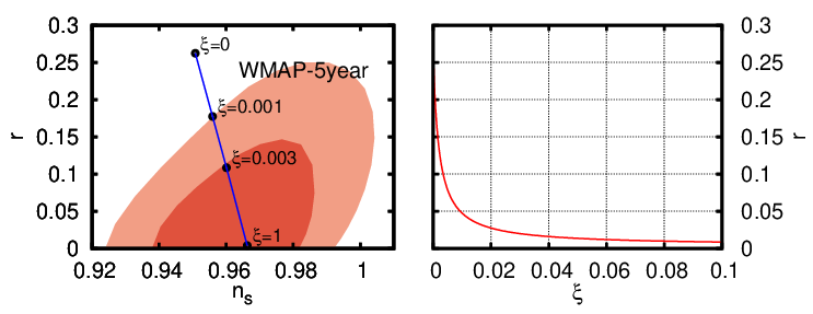
The spectral index and tensor-to-scalar ratio are independent of the coupling constants in the limit of large $\xi$, $n_{s}\simeq 1-8(4N+9)/(4N+3)^{2}\simeq 0.97$, $r\simeq 192/(4N+3)^{2}\simeq 0.0033$. The predicted values are well within one sigma of the current WMAP measurements [7], see Fig. 1.

A very interesting candidate for the inflaton in this case is just the SM Higgs field. Though its self interaction is of the order of unity, sufficiently large $\xi\sim 10^{4}$, (9), allows it to drive inflation, and no new fields have to be added to the SM.

The interesting problem here is the radiative corrections to the potential form the other fields of the SM, like the top quark and the gauge bosons. There are several ways of addressing this problem, that differ by the frame used to define he cut off energy (or normalization point). In [17, 18] the cut off effectively corresponds to constant Planck mass in the Einstein frame, leading to corrections that do not spoil the flatness of the potential (8), while [19] advocates that constant Plank mass cut off should be taken in the Jordan frame, leading to larger corrections, but, interestingly, still allowing for successful inflation, only for rather heavy Higgs mass. The proper way of taking these corrections into account is an important question open for further discussion.

However, large non-minimal coupling $\xi$ is not the only possibility. As far as for zero $\xi$ the amount of tensor modes predicted is too large, and it is very small for large $\xi$, one can ask a question what is the minimal value of $\xi$ that suppresses the tensor mode generation just enough to put them into the WMAP5 preferred region. To answer this question, let us write the expressions for the spectral index and tensor-to-scalar ratio in the limit of small non-minimal coupling constant $\xi$.

The slow roll parameters $\epsilon$ and $\eta$ are [13, 16]

	$$\displaystyle\epsilon={8M_{P}^{4}\over\phi^{2}(M_{P}^{2}+{\xi\phi^{2}(1+6\xi)})}\;,$$		(10)
	$$\displaystyle\eta=\frac{4M_{P}^{2}(3M_{P}^{4}+\xi M_{P}^{2}\phi^{2}(1+12\xi)-2\xi^{2}\phi^{4}(1+6\xi))}{\phi^{2}(M_{P}^{2}+\xi\phi^{2}(1+6\xi))^{2}}\;.$$		(11)

The end of the slow-roll regime ($\epsilon=1$) corresponds to the field value $\phi_{e}$

$$\begin{split}{\xi\phi^{2}_{\mathrm{e}}\over M_{P}^{2}}=&{1\over 2(1+6\xi)}\left(\sqrt{192\xi^{2}+32\xi+1}-1\right)\\ &\approx 8\xi+{\mathcal{O}}(\xi^{2}),~(\xi\ll 1)\;.\end{split}$$

(12)

The number of e-foldings that happened when the field changed its value from $\phi_{N}$ to $\phi_{e}$ is

	$\displaystyle N$	$\displaystyle={1\over M_{P}^{2}}\int^{\phi_{N}}_{\phi_{\mathrm{e}}}{V\over(dV/d\phi)}\left({d\hat{\phi}\over d\phi}\right)^{2}d\phi$		(13)
		$\displaystyle={1\over 8}\left[\frac{\phi_{N}^{2}-\phi^{2}_{\mathrm{e}}}{M_{P}^{2}}(1+6\xi)-6\ln\left({M_{P}^{2}+\xi\phi_{N}^{2}}\over{M_{P}^{2}+\xi\phi^{2}_{\mathrm{e}}}\right)\right]\;.$

For small $\xi\ll 1$ it reduces to $\phi_{N}\simeq\sqrt{8(N+1)}M_{P}$. Then it is easy to calculate the tensor-to scalar ratio [7]

$$\begin{split}r=16\epsilon&={128M_{P}^{4}\over\phi^{2}_{N}(M_{P}^{2}+{\xi\phi^{2}_{N}(1+6\xi)})}\\ &\simeq{16\over(N+1)(1+8(N+1)\xi(1+6\xi))}\;.\end{split}$$

(14)

The spectral index can be obtained as $n_{s}-1=-6\epsilon+2\eta$. The exact formulas are not hard to get by combining (10), (11), (12), and (13), but they are slightly cumbersome and not very instructive, though they were used to plot the figures. Fig. 1 gives the results for several values of $\xi$ together with the WMAP5 preferred region [7]. On can see, that for $\xi>0.001$ and $\xi>0.003$ the predictions enters the $2\sigma$ and $1\sigma$ contours, respectively. The quartic coupling constant $\lambda$ should still be extremely small for these values to satisfy the COBE normalization $U/\epsilon=(0.027M_{P})^{4}$, see Fig. 2.

One can even argue, that for “natural” value for the non-minimal coupling constant of the order of $1$, the amount of tensor perturbations generated is extremely small, so it is natural not to expect the large tensor modes form the inflation, contrary to the usual conclusion for large single field inflation.

We have demonstrated that the non-minimal coupling of the scalar field to gravity loosens the bounds on the field self-coupling constant required for successful inflation, and reduces the amount of tensor modes produced. Large non-minimal coupling (of the order of $10^{4}$) allows to use the SM model Higgs field for inflation. At the same time even very small coupling $\xi\gtrsim 10^{-3}$ makes inflaton with quartic potential compatible with the CMB observations. For the coupling constant $\xi\sim 1$ very small amount of tensor modes is expected for the quartic inflation. Interestingly, that at the same time the non-minimally coupled inflation with quadratic potential and $\xi\sim 1$ is no longer compatible with observations, generating too small spectral index, or even leading potential with runaway behaviour (see [16]).

As a summary, adding non-minimal coupling constant changes the usual expectations from inflation a lot, and lead to interesting predictions. One interesting application to the inflation in the $\nu$MSM model was made in [20].

Author is grateful to M. Shaposhnikov for numerous helpful discussions.

References

- [1] A. A. Starobinsky, JETP Lett. 30, 682 (1979).
- [2] A. A. Starobinsky, Phys. Lett. B91, 99 (1980).
- [3] V. F. Mukhanov and G. V. Chibisov, JETP Lett. 33, 532 (1981).
- [4] A. H. Guth, Phys. Rev. D23, 347 (1981).
- [5] A. D. Linde, Phys. Lett. B108, 389 (1982).
- [6] A. Albrecht and P. J. Steinhardt, Phys. Rev. Lett. 48, 1220 (1982).
- [7] WMAP, E. Komatsu et al., arXiv:0803.0547 [astro-ph].
- [8] A. D. Linde, Phys. Lett. B129, 177 (1983).
- [9] B. L. Spokoiny, Phys. Lett. B147, 39 (1984).
- [10] R. Fakir and W. G. Unruh, Phys. Rev. D41, 1792 (1990).
- [11] D. S. Salopek, J. R. Bond and J. M. Bardeen, Phys. Rev. D40, 1753 (1989).
- [12] D. I. Kaiser, Phys. Lett. B340, 23 (1994), [astro-ph/9405029].
- [13] D. I. Kaiser, Phys. Rev. D52, 4295 (1995), [astro-ph/9408044].
- [14] E. Komatsu and T. Futamase, Phys. Rev. D59, 064029 (1999), [astro-ph/9901127].
- [15] N. D. Birrell and P. C. W. Davies, Quantum Fields in Curved Space (Cambridge, UK: Univ. Pr., 1982).
- [16] S. Tsujikawa and B. Gumjudpai, Phys. Rev. D69, 123523 (2004), [astro-ph/0402185].
- [17] F. L. Bezrukov and M. Shaposhnikov, Phys. Lett. B659, 703 (2008), [arXiv:0710.3755 [hep-th]].
- [18] F. L. Bezrukov, arXiv:0805.2236 [hep-ph].
- [19] A. O. Barvinsky, A. Y. Kamenshchik and A. A. Starobinsky, arXiv:0809.2104 [hep-ph].
- [20] A. Anisimov, Y. Bartocci and F. L. Bezrukov, arXiv:0809.1097 [hep-ph].