Star Formation in the Multiverse

Our goal is not a detailed analytical fit to simulations or observations of the SFR in our universe. Superior models are already available for this purpose. For example, the analytic model of Hernquist and Springel [4] (HS) contains some free parameters, tuned to yield good agreement with simulations and data. However, the HS model only allows for moderate variation in cosmological parameters. For example, HS estimated the SFR in cosmologies with different primordial density contrast, $Q$, but only by 10%.

Here we are interested in much larger variations, by orders of magnitude, and not only in $Q$ but also in the cosmological constant, $\Lambda$, and in spatial curvature. A straightforward extrapolation of the HS model would lead to unphysical predictions in some parameter ranges. For example, a larger cosmological constant would actually enhance the star formation rate at all times [5].¹¹ 1 This effect, while probably unphysical, did not significantly affect the probability distributions computed by Cline et al. [5].

In fact, important assumptions and approximations in the HS model become invalid under large variations of parameters. HS assume a fixed ratio between virial and background density. But in fact, the overdensity of freshly formed haloes drops from about 200 to about 16 after the cosmological constant dominates [6]. Moreover, HS apply a “fresh-halo approximation”, ascribing a virial density and star formation rate to each halo as if it had just been formed. However, large curvature, or a large cosmological constant, will disrupt the merging of haloes. One is left with an old population of haloes whose density was set at a much earlier time, and whose star formation may have ceased due to feedback or lack of baryons. Finally, HS neglect Compton cooling of virialized haloes against the cosmic microwave background; this effect becomes important if structure forms earlier, for example because of increased $Q$ [7].

All these effects are negligible at positive redshift in our universe; they only begin to be important near the present era. Hence, there was no compelling reason to include them in conventional, phenomenologically motivated star formation models. But for different values of cosmological parameters, or when we study the entire evolution of the universe, these effects become important and must be modelled.

On the other hand, some aspects of star formation received careful attention in the HS model in order to optimize agreement with simulations. Such refinements are unnecessary when we work with huge parameter ranges, where uncertainties are large in any case. At best, our goal can be to gain a basic understanding of the quantitative behavior of the SFR as parameters are varied. We will mainly be interested in the height, time, and width of the peak of the SFR depend on parameters. In currently favored models of the multiverse [2, 8], more detailed aspects of the curve do not play an important role. Thus, our model will be relatively crude, even as we include qualitatively new phenomena.

Many extensions of our model are possible. The most obvious is to allow additional parameters to vary. Another is to refine the treatment of star formation itself. Among the many approximations and simplifications we make, the most significant may be our neglect of feedback effects from newly formed stars and from active galactic nuclei. In addition, there are two regimes in our model (high $Q$ and negative $\Lambda$ near the Big Crunch) where we use physical arguments to cut off star formation by hand. These are regimes where the star formation rate is so fast that neglected timescales, such as halo merger rates and star lifetimes, become important. An extended model which accounts for these timescales may avoid the need for an explicit cutoff.

Our star formation model can be applied to open, flat, and closed Friedman-Robertson-Walker (FRW) universes. However, we will consider only open geometries here, with metric

Pocket universes produced by the decay of a false vacuum are open FRW universes [9]; thus, this is the case most relevant to a landscape of metastable vacua. The above metric includes the flat FRW case in the limit where the spatial curvature radius $a$ is much larger than the horizon:

where $H\equiv\dot{a}/a$ is the Hubble parameter. This can be satisfied at arbitrarily late times $t$, given sufficiently many $e$-foldings of slow roll inflation.

The scale factor, $a(t)$, can be computed by integrating the Friedmann equations,

beginning at (matter-radiation) equality, the time $t_{\rm eq}$ at which matter and radiation have equal density:

where

accounts for three species of massless neutrinos. The temperature at equality is [6]

and $\xi$ is the matter mass per photon. The time of equality is

The total density and pressure are given by

Among the set of initial data specified at equality, we will treat three elements as variable parameters, which define an ensemble of universes. The first two parameters are the densities associated with curvature, $G_{\rm N}^{-1}a(t_{\rm eq})^{-2}$, and with the vacuum, $\rho_{\Lambda}\equiv\Lambda/8\pi G_{\rm N}$, at equality. We will only consider values that are small compared to the radiation and matter density at equality, Eq. (5); otherwise, there would be no matter dominated era and no star formation. The third parameter is the primordial density contrast, $Q$, discussed in more detail in the next section.

We find it intuitive to trade the curvature parameter $a(t_{\rm eq})$ for an equivalent parameter $\Delta N$, defined as

where

is the experimental lower bound on the curvature radius of our universe at matter-radiation equality. (Consistency with our earlier assumption of an open universe requires that we use the upper bound on negative spatial curvature, i.e., on positive values of $\Omega_{k}$. We are using the 68% limit from WMAP5+BAO+SN [10], $\Omega_{k}=-0.0050^{+0.0061}_{-0.0060}$. We use the best fit values $H_{0}=68.8~\mbox{km/s/Mpc}$ and $\Omega_{\rm m}=0.282$ for the current Hubble parameter and matter density fraction.)

$\Delta N$ can be interpreted as the number of $e$-folds of inflation in excess (or short) of the number required to make our universe (here assumed open) just flat enough ($\Omega^{\rm max}_{k}=0.0011$) for its spatial curvature to have escaped detection. Requiring that curvature be negligible at equality constrains $\Delta N$ to the range $\Delta N>-5$. Values near this cutoff are of no physical interest in any case: Because too much curvature disrupts galaxy formation, we will find that star formation already becomes totally ineffective below some larger value of $\Delta N$.

We hold fixed all other parameters, including Standard Model parameters, the baryon to dark matter ratio, and the temperature at equality. We leave the variation of such parameters to future work.

Cosmological perturbations are usually specified by a time-dependent power spectrum, $\mathcal{P}$, which is a function of the wavenumber of the perturbation, $k$. The r.m.s. fluctuation amplitude, $\sigma$, within a sphere of radius $R$, is defined by smoothing the power spectrum with respect to an appropriate window function:

The radius $R$ can be exchanged for the mass $M$ of the perturbation, using $M=4\pi\rho_{\rm m}R^{3}/3$. Starting at $t_{\rm eq}$, once all relevant modes are in the horizon, the time development of $\sigma$ can be computed using linear perturbation theory. In the linear theory, all modes grow at the same rate and so the time dependence of $\sigma$ is a simple multiplicative factor:

Here $Q$ is the amplitude of primordial density perturbations, which in our universe is observed to be $Q_{0}\approx 2\times 10^{-5}$. $G(t)$ is the linear growth function, and is found by solving

numerically, with the initial conditions $G=5/2$ and $\dot{G}=3H/2$ at $t=t_{\rm eq}$. This normalization is chosen so that $G\approx 1+\frac{3}{2}\frac{a(t)}{a(t_{\rm eq})}$ near $t=t_{\rm eq}$, which is the exact solution for a flat universe consisting only of matter and radiation. For $s(M)$ we use the fitting formula provided in [6]:

with $\mu=M/M_{\rm eq}$, where

is roughly the mass contained inside the horizon at equality, and $\xi=3.7$ eV is the matter mass per photon. This fitting formula for $s(M)$ and our normalization convention for $G(t)$ both make use of our assumption that curvature and $\rho_{\Lambda}$ are negligible at $t_{\rm eq}$.

We use the extended Press-Schechter (EPS) formalism [11] to estimate the halo mass function and the distribution of halo ages. In this formalism the fraction, $F$, of matter residing in collapsed regions with mass less than $M$ at time $t$ is given by

with $\delta_{\rm c}=1.68$ the critical fluctuation for collapse. $\delta_{\rm c}$ is weakly dependent on cosmological parameters, but the variation is small enough to ignore within our approximations.

Given a halo of mass $M$ at time $t$, one can ask for the probability, $P$, that this halo virialized before time $t_{\rm vir}$. As in Ref. [11], we define the virialization time of the halo as the earliest time when its largest ancestor halo had a mass greater than $M/2$. To find $P$, we first define the function

Then the desired probability is given by

The virialization time further determines the density, $\rho_{\rm vir}$, of the halo. We will compute the virial density by considering the spherical top-hat collapse of an overdense region of space. Birkhoff’s theorem says that we may consider this region to be part of an independent FRW universe with a cosmological constant identical to that of the background universe. As such, it evolves according to

where $A\equiv\left(\frac{|\rho_{\Lambda}|}{\rho_{\rm m}}\right)^{1/3}$ and $\kappa\equiv\frac{3}{8\pi G_{\rm N}|\rho_{\Lambda}|}\left(\frac{A}{a}\right)^{2}k$. We neglect the radiation term, which will be negligible for virialization well after matter-radiation equality.

Assuming that $\kappa$ and $\rho_{\Lambda}$ are such that the perturbation will eventually collapse, the maximum value of $A$ is obtained by solving the equation $H=0$:

The time of collapse, which we identify with the halo virialization time $t_{\rm vir}$, is twice the time to reach $A_{\rm max}$ and is given by

To obtain the virial density, we follow the usual rule that $\rho_{\rm vir}$ is $8$ times the matter density at turnaround. In other words,

Note that according to this prescription, $\rho_{\rm vir}(t)$ has no explicit dependence on the curvature of the background universe. Changing $\rho_{\Lambda}$ results in a simple scaling behavior: $\rho_{\rm vir}(t/t_{\Lambda})/|\rho_{\Lambda}|$ is independent of $\rho_{\Lambda}$, where

In practice this means that one only has to compute $\rho_{\rm vir}(t)$ for two values of $\rho_{\Lambda}$ (one positive and one negative). In Fig. 1, we show the $\rho_{\Lambda}$-independent part of the virial density.

The virial density determines the gravitational timescale, $t_{\rm grav}$, which we define to be

This is the timescale for dynamical processes within the halo, including star formation.

Halos typically virialize at a high temperature, $T_{\rm vir}$. Before stars can form, the baryons need to cool to lower temperatures and condense. Cooling proceeds by bremsstrahlung, molecular or atomic line cooling, and Compton cooling via scattering against the CMB.

For bremsstrahlung and line cooling, the timescale for the baryons to cool, $t_{\rm cool}$, is

with $\mu=0.6\,m_{\rm p}$ the average molecular weight (assuming full ionization), $X=.76$ the hydrogen mass fraction, and $\Lambda(T_{\rm vir})$ the cooling function, which encodes the efficiency of the bremsstrahlung and line cooling mechanisms as a function of temperature. For $T\lesssim 10^{4}\,{\rm K}$, $\Lambda(T)$ is effectively zero and cooling does not occur. When $T\gtrsim 10^{7}\,{\rm K}$, bremsstrahlung cooling is the dominant mechanism and $\Lambda(T)\propto T^{1/2}$. For intermediate values of $T$, $\Lambda(T)$ has a complicated behavior depending on the metallicity of the gas [12]. For our purposes, however, it suffices to approximate the cooling function as constant in this range. To summarize:

with $\Lambda_{0}=10^{-23}{\rm erg}\,{\rm cm}^{3}\,{\rm s}^{-1}$.

We need to include the effects of Compton cooling separately. In general, Compton cooling depends on the temperature of the CMB, $T_{\rm CMB}$, the temperature of the baryonic matter, and the ionization fraction of the matter [13]. But the dependence on the gas temperature drops out when $T_{\rm vir}\gg T_{\rm CMB}$ (which is always the case), and we will assume that the gas transitions from neutral to completely ionized at $T_{\rm vir}=10^{4}\,{\rm K}$. With these approximations, Compton cooling proceeds along the timescale

where $\sigma_{\rm T}=\frac{8\pi}{3}\left(\frac{e^{2}}{m_{\rm e}}\right)^{2}$ is the Thompson cross-section.

The Compton timescale is independent of all of the properties of the gas (provided $T_{\rm vir}>10^{4}{\rm K}$). So this cooling mechanism can still be efficient in regimes where other cooling mechanisms fail. In particular, Compton cooling will be extremely effective in the early universe while the CMB is still hot. We define $\tau_{\rm comp}$ as the time when $t_{\rm comp}$ is equal to the age of the universe. $\tau_{\rm comp}$ is a reasonable convention for the time beyond which Compton cooling is no longer efficient. While we compute $\tau_{\rm comp}$ numerically in practice, it is helpful to have an analytic formula for a special case. In a flat, $\rho_{\Lambda}=0$ universe we obtain

Turning on strong curvature or $\rho_{\Lambda}$ will tend to lower $\tau_{\rm comp}$.

Before $\tau_{\rm comp}$, all structures with $T_{\rm vir}>10^{4}{\rm K}$ can cool efficiently and rapidly, so star formation will proceed on the timescale $t_{\rm grav}$. After $\tau_{\rm comp}$, some halos will have $t_{\rm cool}<t_{\rm grav}$ and hence cool efficiently, and some will have $t_{\rm cool}>t_{\rm grav}$ and be “cooling-limited”. We take it as a phenomenological fact that the cooling-limited halos do not form stars. (One could go further and define a “cooling radius” to take into account the radial dependence of the baryonic density [13], but this effect is negligible within our approximations.)

In the absence of Compton cooling, then, we will consider only halos for which $t_{\rm cool}<t_{\rm grav}$, which have masses in a finite range:

The minimum halo mass at time $t_{\rm vir}$ corresponds to the minimum temperature $T_{\rm vir}=10^{4}{\rm K}$:

where we have used the relation between virial temperature, density, and mass for a uniform spherical halo derived from the virial theorem:

(A non-uniform density profile will result in a change to the numerical factor on the RHS of this equation, but such a change makes little difference to the result.)

The maximum mass haloes at time $t_{\rm vir}$ satisfy $t_{\rm cool}=t_{\rm grav}$. For $T<10^{7}{\rm K}$, this mass is given by

Note that halos with mass $M_{\rm max}(t)$ have virial temperatures less than $10^{7}{\rm K}$ for $t\gtrsim 0.24\,{\rm Gyr}$, which is well before $\tau_{\rm comp}$. This means that in our calculations we can safely ignore the decreased cooling efficiency for extremely hot halos.

For halos satisfying the criterion $t_{\rm cool}<t_{\rm grav}$, the hot baryonic material is allowed to cool. Gravitational collapse proceeds on the longer timescale $t_{\rm grav}$. We will assume that the subsequent formation of stars is also governed by this timescale. Thus, we write the star formation rate for a single halo of mass $M$ as

where $M_{\rm b}$ is the total mass of baryons contained in the halo and $f_{\rm b}$ is the baryon mas fraction. We fix $f_{\rm b}$ to the observed value $f_{\rm b}\approx 1/6$.²² 2 It would be interesting to consider variations of $f_{\rm b}$ in future work; see Ref. [14] for an environmental explanation of the observed value.

The order-one factor $A$ parametrizes the detailed physics of gravitational collapse and star formation. The free-fall time from the virial radius to a point mass $M$ is $(3\pi/32)^{1/2}\,t_{\rm grav}$, and so we choose to set $A=(32/3\pi)^{1/2}$. The final SFR calculated for our universe is not very sensitive to this choice. Notice that the single halo star formation rate depends only on the mass and virialization time of the halo.

The next step in computing the complete SFR is to average over the virialization times of the halos in existence at time $t$. Define $\frac{dM_{\star}^{\rm avg}}{dt}(M,t)$ to be the star formation rate of all halos that have mass $M$ at time $t$, averaged over possible virialization times $t_{\rm vir}$. Now we need to consider the possible virialization times.

It may happen that some halos in existence at time $t$ are so old that they have already converted all of their baryonic mass into stars. These halos should not be included in the calculation. Furthermore, feedback effects reduce the maximum amount of baryonic matter that can ever go into stars to some fraction $f$ of the total. ($f$ is a free parameter of the model, and we shall fix its value by normalizing the integrated SFR for our universe; see below.) We should then only consider halos with $t_{\rm vir}>t_{\rm min}$, where $t_{\rm min}$ is a function of $t$ only and satisfies

Though an explicit expression for $t_{\rm min}$ can be found in some special cases, in practice we will always solve for it numerically.

We still need to account for the fact that some halos existing at $t$ formed at $t_{\rm vir}$ with masses outside the range $M_{\rm min}(t_{\rm vir})<M<M_{\rm max}(t_{\rm vir})$. Since $M_{\rm min}$ is an increasing function of time while $M_{\rm max}$ is a decreasing function of time, this condition on the mass range is equivalent to an upper bound on $t_{\rm vir}$: $t_{\rm vir}<t_{\rm max}$, where $t_{\rm max}$ satisfies either

or

or else $t_{\rm max}=t$ if no solution exists. Recall that the condition $M<M_{\rm max}$ is a condition on cooling failure, and so is only applicable for $t_{\rm vir}>\tau_{\rm comp}$. Halos with $t_{\rm vir}<\tau_{\rm comp}$ have no upper mass limit. Like $t_{\rm min}$, $t_{\rm max}$ is found numerically. Unlike $t_{\rm min}$, $t_{\rm max}$ is a function of both mass and time.

Now we can use the distribution on halo formation times deduced from Eq. 20 to get

The final step is to multiply this average by the number of halos of mass $M$ existing at time $t$ and add up the contributions from all values of $M$. Equivalently, we can multiply the normalized average star formation rate, $\frac{1}{M}\frac{dM_{\star}^{\rm avg}}{dt}$, by the total amount of mass in halos of mass $M$ at time $t$ and then add up the contributions from the different mass scales. The Press-Schechter formalism tells us that the fraction of the total mass contained in halos of masses between $M$ and $M+dM$ is $\frac{\partial F}{\partial M}dM$, where $F(M,t)$ is the Press-Schechter mass function defined in Eq. 18. So restricting ourselves to a unit of comoving volume with density $\rho_{0}$ (sometimes called the reference density), we find that the SFR is given by

We begin by considering our own universe. Figure 2 shows the SFR computed by our model as a function of time (left) and of redshift (right). At intermediate redshifts, our model is in good agreement with the data. At other redshifts, our model appears to be slightly off, but not by a large factor, considering its crudeness. For comparison, we show the SFR predicted by the models of HS [4], Nagamine et al. [15] and Hopkins and Beacom [16], which contain a larger number of fitting parameters.

The shape of the SFR can be understood as a result of the interplay between competing forces. First, there will be no star formation until structure forms with $T_{\rm vir}>10^{4}{\rm K}$. Once a significant amount of structure begins to form at this critical temperature, however, the SFR rises rapidly and soon hits its peak.

We can estimate the peak time, $t_{\rm peak}$, of the SFR by asking when the typical mass scale that virializes is equal to $M_{\rm min}$:

(There are ambiguities at the level of factors of order one; the factor $\sqrt{2}$ was chosen to improve agreement with the true peak time of the SFR.) For the parameters of our universe, this calculation yields $t_{\rm peak}=1.7\,\mbox{Gyr}$, close to the peak predicted by our model at about $1.6\,\mbox{Gyr}$.

After $t\approx t_{\rm peak}$, the SFR falls at least as fast as $1/t$ because $t_{\rm grav}\propto t$. Once the typical virialized mass exceeds the cooling limit, $M_{\rm max}$, the SFR falls faster still. These considerations generalize to universes besides our own after accounting for the peculiar effects of each of the cosmological parameters. In particular, as explained below, we should be able to accurately estimate the peak time by this method for any universe where the effects of curvature or the cosmological constant are relatively weak.

Next, we present several examples of star formation rates computed from our model for universes that differ from ours through a single parameter.

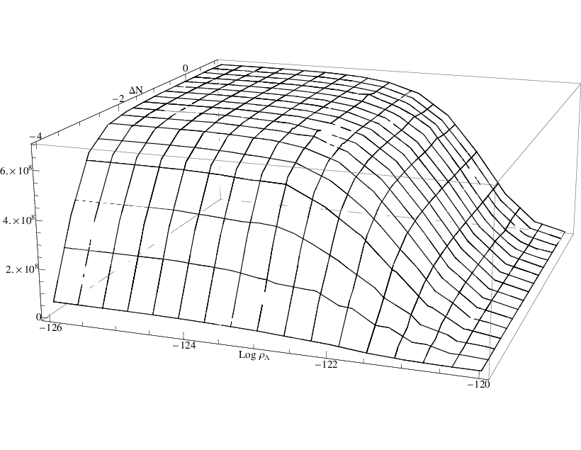
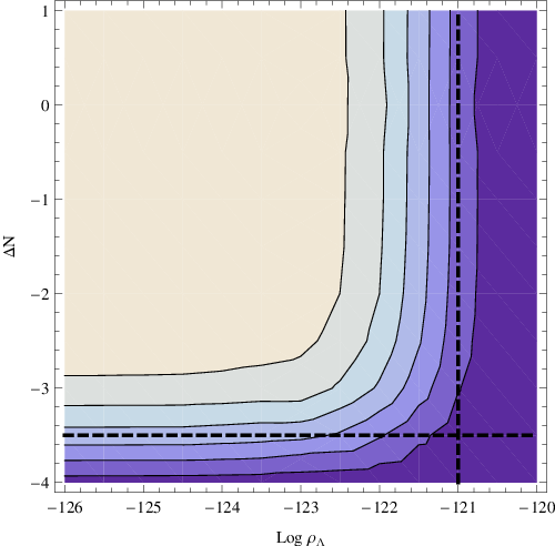
We can also vary multiple parameters at once. For example, let us hold only $Q$ fixed and vary both curvature and (positive) vacuum energy. The integrated star formation is is shown in Fig. 8. If either curvature or $\rho_{\Lambda}$ get large, then structure formation is suppressed and star formation goes down. When the universe has both small $\rho_{\Lambda}$ and small curvature, then structure formation is not suppressed and the SFR is nearly identical to that of our universe. Here “large” and “small” should be understood in terms of the relation between $t_{\Lambda}$, $t_{\rm c}$, and $t_{\rm peak}$ computed in a flat, $\rho_{\Lambda}=0$ universe (an unsuppressed universe). In the case we are considering, namely $Q=Q_{0}$, the unsuppressed peak time is $t_{\rm peak}=1.7\,\mbox{Gyr}$. The conditions $t_{\rm peak}=t_{\Lambda}$ and $t_{\rm peak}=t_{\rm c}$ translate into $\rho_{\Lambda}\approx 100\,\rho_{\Lambda_{0}}$ and $\Delta N\approx-3.5$ . These lines are marked in Fig. 8, and one sees that this is a good approximation to the boundary of the star-forming region. (We will see below that this approximation does not continue to hold if both curvature and $Q$ are allowed to vary.)

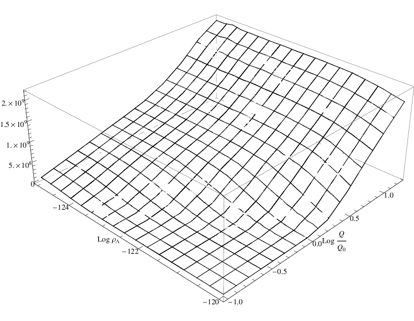
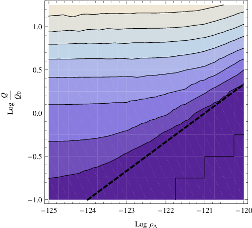
If we also start to vary $Q$, the story gets only slightly more complicated. Increasing $Q$ causes structure formation to happen earlier, resulting in more star formation. In the multivariate picture, then, it is helpful to think of $Q$ as changing the unsuppressed $t_{\rm peak}$. For the unsuppressed case, the universe can be approximated as matter-dominated. Looking at Eq. 43 and recalling that $G\sim a\propto t^{2/3}$ in a matter-dominated universe, and neglecting for the sake of computational ease the dependence on $M_{\rm min}$, we see that $t_{\rm peak}\propto Q^{-3/2}$. Now we can quantitatively assess the dependence of star formation on $Q$ and $\rho_{\Lambda}$, for instance. We know that $t_{\Lambda}=t_{\rm peak}$ when $Q=Q_{0}$ and $\rho_{\Lambda}=100\,\rho_{\Lambda_{0}}$, and this condition should generally mark the boundary between star formation and no star formation. Therefore we can deduce that the boundary in the two-dimensional parameter space is the line $\log_{10}\rho_{\Lambda}/\rho_{\Lambda_{0}}=2+3\log_{10}Q/Q_{0}$ . This line is shown in Fig. 9, where it provides a good approximation to the failure of star formation.

We can repeat the same analysis for the case of fixed cosmological constant with varying curvature and perturbation amplitude. In Fig. 10 we show the integrated star formation rate as a function of $\Delta N$ and $Q$ for fixed $\rho_{\Lambda}=\rho_{\Lambda_{0}}$. The dashed line in Fig. 10 marks the boundary $t_{\rm c}=t_{\rm peak}$, where the time of curvature domination equals the time of the unsuppressed peak (again computed according to Eq. 43). In this case the line is given by $(2\Delta N+7)\log_{10}e=-\log_{10}Q/Q_{0}$, owing to the fact that $t_{\rm c}\propto\exp(3\Delta N)$. Unlike the case of $\rho_{\Lambda}$, this line obviously does not mark the transition from structure formation to no structure formation. The reason has to do with the details of the nature of the suppression coming from curvature versus that coming from the cosmological constant. In the case of the cosmological constant, it is a very good approximation to say that structure formation proceeds as if there were no cosmological constant up until $t=t_{\Lambda}$, whereupon it stops suddenly. Curvature is far more gradual: its effects begin well before $t_{\rm c}$ and structure formation continues well after $t_{\rm c}$. Fig. 11 illustrates this point clearly. There we see that while perturbations are suppressed in both the high curvature and large $\rho_{\Lambda}$ cases, it is only in the $\rho_{\Lambda}$ case that the naive approximation of a “sudden end” to structure formation is valid. For the curvature case there is no simple approximation, and the full model is necessary to give an accurate assessment of the situation.