跳到论文正文
W Papers独立论文阅读器 arXiv:0810.3027 论文正文 计算阅读时间 · 0%
引用这篇论文根据当前论文元数据生成,正式投稿前建议核对。


License: arXiv.org perpetual non-exclusive license
arXiv:0810.3027v1 [math.CV] 16 Oct 2008

Behavior of lacunary series at the natural boundary

O. Costin, M. Huang Address: Mathematics Department//The Ohio State University//Columbus, OH 43220
Abstract.

We develop a local theory of lacunary Dirichlet series of the form ∑k=1∞ck​exp⁡(−z​g​(k)),Re⁡(z)>0\sum\limits_{k=1}^{\infty}c_{k}\exp(-zg(k)),\mathrm{Re}(z)>0 as zz approaches the boundary i​ℝi\mathbb{R}, under the assumption g′→∞g^{\prime}\to\infty and further assumptions on ckc_{k}. These series occur in many applications in Fourier analysis, infinite order differential operators, number theory and holomorphic dynamics among others. For relatively general series with ck=1c_{k}=1, the case we primarily focus on, we obtain blow up rates in measure along the imaginary line and asymptotic information at z=0z=0.

When sufficient analyticity information on gg exists, we obtain Borel summable expansions at points on the boundary, giving exact local description. Borel summability of the expansions provides property-preserving extensions beyond the barrier.

The singular behavior has remarkable universality and self-similarity features. If g⁡(k)=kbg(k)=k^{b}, ck=1c_{k}=1, b=nb=n or b=(n+1)/nb=(n+1)/n, n∈ℕn\in\mathbb{N}, behavior near the boundary is roughly of the standard form Re​(z)−b′​Q​(x)\mathrm{Re}(z)^{-b^{\prime}}Q(x) where Q⁡(x)=1/qQ(x)=1/q if x=p/q∈ℚx=p/q\in\mathbb{Q} and zero otherwise.

The Bötcher map at infinity of polynomial iterations of the form xn+1=λ​P​(xn)x_{n+1}=\lambda P(x_{n}), |λ|<λ0​(P)|\lambda|<\lambda_{0}(P), turns out to have uniformly convergent Fourier expansions in terms of simple lacunary series. For the quadratic map P⁡(x)=x−x2P(x)=x-x^{2}, λ0=1\lambda_{0}=1, and the Julia set is the graph of this Fourier expansion in the main cardioid of the Mandelbrot set.

1. Introduction

Natural boundaries (NBs) occur frequently in many applications of analysis, in the theory of Fourier series, in holomorphic dynamics (see [8], [7], [5] and references there), in analytic number theory, see [20], physics, see [13] and even in relatively simple ODEs such as the Chazy equation [11], an equation arising in conformal mapping theory, or the Jacobi equation.

The intimate structure of NBs turns out to be particularly rich, bridging analysis, number theory and complex dynamics.

Nonetheless (cf. also [13]), the study of NBs of concrete functions is yet to be completed from a pure analytic point of view. The aim of the present paper is a detailed study near the analyticity boundary of a prototypical functions exhibiting this singularity structure, classes of lacunary series. For such functions, we develop a theory of generalized local asymptotic expansions at NBs, and explore their consequences and applications. The expansions are asymptotic in the sense that they become increasingly accurate as the singular curve is approach, and in many cases exact, in that the function can be recovered from these expansions.

Lacunary series, sums of the form h⁡(s)=∑j≥1cj​sgjh(s)=\sum_{j\geq 1}{c_{j}}s^{g_{j}}, or written as Dirichlet series f⁡(z)=∑j≥1cj​e−z​g​(j)f(z)=\sum_{j\geq 1}{c_{j}}e^{-z{g(j)}}), where j/gj=o⁡(1)j/g_{j}=o(1) for large jj, often occur in applications and have deep connections with infinite order differential operators, as found and studied by Kawai [12], [13]. Under the lacunarity assumption above, if the unit disk is the maximal disk of analyticity of hh, then the unit circle is its NB ([15]). For instance, the series

h⁡(s)=∑j=1∞s2j​(|s|<1)h(s)=\sum_{j=1}^{\infty}s^{2^{j}}\>(|s|<1) (1)

studied by Jacobi [10] before the advent of modern Complex Analysis, clearly has the unit disk as a singular curve: h⁡(s)→+∞h(s)\to+\infty as |s|↑1|s|\uparrow 1 along any ray of angle 2−n​m​π2^{-n}m\pi with m,n∈ℕm,n\in\mathbb{N}.

We show that if cj=1c_{j}=1 and g′→∞g^{\prime}\to\infty, then, in a measure theoretic sense, f⁡(x+i​y)f(x+iy) blows up as x→0+x\to 0^{+} uniformly in yy at a calculable rate. We find interesting universality properties in the blow-up profile.

In special cases of interest, Borel summable power series, in powers of the distance to the boundary, and more generally convergent expansions as series of small exponentials multiplying Borel summed series power series11 1 These are simple instances of Borel (or Ecalle-Borel) summed transseries. A brief summary of the definitions and properties of transseries and generalized Borel summability, and references to the literature are given in §5.6. representations can be determined on a dense set on the singularity barrier. Examples are

  • •

    ∑j≥1e−z​jb\sum_{j\geq 1}e^{-zj^{b}} where b>1b>1, or its dual q>1q>1, where b−1+q−1=1b^{-1}+q^{-1}=1, is integer (relating to exponential sums and van der Corput dualities [17]; the special self-dual case ∑j≥1e−z​j2\sum_{j\geq 1}e^{-zj^{2}}, is related to the Jacobi theta function);

  • •

    ∑j≥1e−z​aj\sum_{j\geq 1}e^{-za^{j}}, 1<a∈ℕ1<a\in\mathbb{N};

More generally, if cj=c⁡(j)c_{j}=c(j) and gj=g⁡(j)g_{j}=g(j) have suitable analyticity properties in jj, then the behavior at z=0+z=0^{+}, and possibly at other points, is described in terms of Ecalle-Borel summed expansions (see footnote 1). Then the analysis leads to a natural, properties-preserving, continuation formulas across the boundary.

In general, the blow-up profile along the barrier is closely related to exponential sums, expressions of the form

SN=∑k=1Ncn​exp⁡(2​π​i​g​(n)),g⁡(n)∈ℝS_{N}=\sum_{k=1}^{N}c_{n}\exp(2\pi ig(n)),\ \ g(n)\in\mathbb{R} (2)

where for us g′→∞g^{\prime}\to\infty as n→∞n\to\infty. The corresponding lacunary series are in a sense the continuation of (2) in the complex domain, replacing 2​π​i2\pi i by −z-z, Re⁡(z)>0\mathrm{Re}(z)>0, and letting N→∞N\to\infty. The asymptotic behavior of lacunary series as the imaginary line is approached in nearly-tangential directions is described by dual, van der Corput-like, expansions. The method we use extend to exponential sums, which will be the subject of a different paper.

2. Results

2.1. Results under general assumptions

2.1.1. Blow-up on a full measure set

We consider lacunary Dirichlet series of the form

f⁡(z)=∑k=0∞e−z​g​(k)f(z)=\sum_{k=0}^{\infty}e^{-zg(k)} (3)

but, as it can be seen from the proofs, the analysis extends easily to series of the form

f⁡(z)=∑j=0∞cj​e−z​g​(j)f(z)=\sum_{j=0}^{\infty}c_{j}e^{-zg(j)}

under suitable smoothness and growth conditions, see §3.8. The results in the paper apply under the further restriction,

Assumption 1.

The function gg is differentiable and g′​(j)→∞g^{\prime}(j)\to\infty as j→∞j\to\infty.

In particular, gg is eventually increasing. By subtracting a finite sum of terms from ff (a finite sum is clearly entire), we arrange that gg is increasing. If g⁡(0)=ag(0)=a, we can multiply ff by e−z​ae^{-za} to arrange that g⁡(0)=0g(0)=0.

Normalization 1.

(i) gg is differentiable on [0,∞)[0,\infty), g′>0g^{\prime}>0 and g′→∞g^{\prime}\to\infty along ℝ+\mathbb{R}^{+}.

(ii) g⁡(0)=0g(0)=0.

Notation. We write |H⁡(⋅)|​=μ1+o⁡(1)\displaystyle|H(\cdot)|\mathop{=}^{\mu}1+o(1) if |H⁡(y)|​d​y|H(y)|dy converges to the Lebesgue measure d​μ​(y)d\mu(y).

Under Assumption 1, after normalization, we have the following result, giving exact blow-up rates in measure, as well as sharp pointwise blow-up upper bounds.

Theorem 1.

(i) We have the uniform blow-up rate in measure22 2 It turns out that in general, L1L^{1} or a.e. convergence of |f||f| do not hold..

|f(x+i⋅)|2=μ∫0∞e−2​g​(s)​xds(1+o(1))|f(x+i\cdot)|^{2}\mathop{=}^{\mu}\int_{0}^{\infty}e^{-2g(s)x}ds\left(1+o(1)\right) (4)

It can be checked that ∫0∞e−2​g​(s)​x​𝑑s≥g−1​(1/x)→∞​ as ​x→0+\int_{0}^{\infty}e^{-2g(s)x}ds\ \geq g^{-1}(1/x)\to\infty{\text{ as }}x\to 0^{+}; see also Note 1.

(ii) The following pointwise estimate holds:

∥f(x+i⋅)∥∞≤∫0∞e−g⁡(s)​xds(1+o(1))as x→0+\|f(x+i\cdot)\|_{\infty}\leq\int_{0}^{\infty}e^{-g(s)x}ds(1+o(1))\ \ \text{as }x\to 0^{+} (5)

This is sharp at z=0z=0, cf. Proposition 2, and in many cases it is only reached at z=0z=0; see Proposition 5.

2.1.2. General behavior near z=0z=0

At z=0+z=0^{+} a more detailed asymptotic description is possible.

Theorem 2.

(i) As z→0+z\to 0^{+} we have

f⁡(z)=∫0∞e−z​g​(s)​𝑑s−12+o⁡(1)→∞as ​z→0+f(z)=\int_{0}^{\infty}e^{-zg(s)}ds-\frac{1}{2}+o(1)\ \to\infty\ \ \ \text{as }z\to 0^{+} (6)

In fact,

f(z)−∫0∞e−z​g​(s)ds=−z∫0∞e−z​u{g−1(u)}duf(z)-\int_{0}^{\infty}e^{-zg(s)}ds=-z\int_{0}^{\infty}e^{-zu}\{g^{-1}(u)\}du (7)

(where {⋅}\{\cdot\} denotes the fractional part, and we used g⁡(0)=0g(0)=0)33 3 As mentioned, often this maximal growth is achieved at zero but in special cases it occurs, up to a bounded function, on a dense set of measure zero..

(ii) If g⁡(s)g(s) has a differentiable asymptotic expansion as s→∞s\to\infty in terms of (integer or noninteger) powers of ss and log⁡s\log s, and g⁡(s)∼c​o​n​s​t.sbg(s)\sim const.s^{b}, b>1b>1, then after subtracting the blowing up term, ff has a Taylor series at z=0z=0 (generally divergent, even when gg is analytic, which can be calculated explicitly),

f(z)=∫0∞e−z​g​(s)ds−12+zs(z),s∈C∞[0,∞)f(z)=\int_{0}^{\infty}e^{-zg(s)}ds-\frac{1}{2}+zs(z),\ \ s\in C^{\infty}[0,\infty)

(as an example, see (61).

Note 1.

Often gg has an asymptotic expansion starting with a combination of powers, exponentials and logs. Let ϕ=g−1\phi=g^{-1}. Then ϕ⁡(ν​x)/ϕ⁡(ν)→ϕ1​(x)\phi(\nu x)/\phi(\nu)\to\phi_{1}(x) as ν→∞\nu\to\infty and x>0x>0 is fixed and

∫0∞e−x​g​(s)​𝑑s=Cg​g−1​(1/x)​(1+o⁡(1));Cg=∫0∞e−u​ϕ1​(u)​𝑑u\int_{0}^{\infty}e^{-xg(s)}ds=C_{g}g^{-1}(1/x)(1+o(1));\ \ \ C_{g}=\int_{0}^{\infty}e^{-u}\phi_{1}(u)du

For instance, if g⁡(k)=kb,b>1g(k)=k^{b},b>1 we have, as ρ→1\rho\to 1,

|f(z)|=μx−12​bΓ(1+1/b)−1/22−12​b(1+o(1))(x→0+)\displaystyle|f(z)|\mathop{=}^{\mu}x^{-\frac{1}{2b}}\,\,\Gamma(1+1/b)^{-1/2}2^{-\frac{1}{2b}}(1+o(1))\ \ \ (x\to 0^{+})
f⁡(x)=x−1b​Γ​(1+1/b)​(1+o⁡(1))(x→0+)\displaystyle f(x)=x^{-\frac{1}{b}}\,\,\Gamma(1+1/b)(1+o(1))\ \ \ \ \ \ \ (x\to 0^{+}) (8)

2.1.3. Blow-up profile along barrier

Theorem 3.

(i) Assume that for some y∈ℝy\in\mathbb{R} there is a smooth increasing function ρ⁡(N,y)=:ρ⁡(N)∈(0,N]\rho(N;y)=:\rho(N)\in(0,N] such that the following weighted exponential sum (see [17]) has a limit:

Sρ,N:=ρ​(N)−1​∑j=1Nei​y​g​(j)→L⁡(y)asN→∞S_{\rho,N}:=\rho(N)^{-1}\sum_{j=1}^{N}e^{iyg(j)}\to L(y)\ \ \text{as}\ \ N\to\infty (9)

where ρ′′\rho^{\prime\prime} is uniformly bounded and nonpositive for sufficiently large kk. (Without loss of generality, we may assume ρ′′​(k)≤0\rho^{\prime\prime}(k)\leq 0 for all kk.) Let

Φ⁡(x)=∫0∞e−x​g​(u)​ρ′​(u)​𝑑u\Phi(x)=\int_{0}^{\infty}e^{-xg(u)}\rho^{\prime}(u)du (10)

Then, we have the asymptotic behavior

f⁡(x+i​y)=L⁡(y)​Φ​(x)+o⁡(Φ⁡(x))(x→0+)f(x+iy)=L(y)\Phi(x)+o(\Phi(x))\ \ \ (x\to 0^{+}) (11)

(ii) As a pointwise upper bound we have:

lim supN≥0|Sρ,N|=L<∞⇒f⁡(x+i​y)=O⁡(Φ⁡(x))(x→0+)\limsup_{N\geq 0}|S_{\rho,N}|=L<\infty\ \Rightarrow\ f(x+iy)=O(\Phi(x))\ \ \ (x\to 0^{+}) (12)

2.2. Results in specific cases

2.2.1. Settings leading to convergent expansions

The cases g⁡(j)=j2g(j)=j^{2} and g⁡(j)=ajg(j)=a^{j}, a>1a>1 are distinguished, since the expansions at some points near the boundary converge.

Proposition 1.

If b=2b=2, then we have the identity

f⁡(z)=12​πz−12+πz​∑k=1∞e−k2​π2zf(z)=\frac{1}{2}\sqrt{\frac{\pi}{z}}-\dfrac{1}{2}+\sqrt{\frac{\pi}{z}}\sum_{k=1}^{\infty}e^{-\frac{k^{2}\pi^{2}}{z}}

Clearly, this is most useful when z→0z\to 0. It also shows the identity associated to the Jacobi theta function

f⁡(z)=12​πz−12+πz​f​(k2​π2z)f(z)=\frac{1}{2}\sqrt{\frac{\pi}{z}}-\dfrac{1}{2}+\sqrt{\frac{\pi}{z}}f\left(\frac{k^{2}\pi^{2}}{z}\right) (13)
Proposition 2.

If g⁡(j)=ajg(j)=a^{j}, a>1a>1, then, as z→0+z\to 0^{+}, f⁡(z)f(z) is convergently given by

f⁡(z)=−log⁡ζlog⁡a+∑n=1∞(−ζ)nn!​(1−an)+c0+1log⁡a​∑k≠0Γ⁡(−2​k​π​ilog⁡a)​ζ2​k​π​ilog⁡a=−log⁡ζlog⁡a+∑n=1∞(−ζ)nn!​(1−an)+c0−12​π​i​∫0∞logℝ⁡[−(s/ζ)2​π​ilog⁡a]​e−s​𝑑sf(z)=-\dfrac{\log\zeta}{\log a}+\sum_{n=1}^{\infty}\frac{(-\zeta)^{n}}{n!(1-a^{n})}+c_{0}+\frac{1}{\log a}\sum_{k\neq 0}\Gamma\left(-\frac{2k\pi i}{\log a}\right)\zeta^{\frac{2k\pi i}{\log a}}\\ =-\dfrac{\log\zeta}{\log a}+\sum_{n=1}^{\infty}\frac{(-\zeta)^{n}}{n!(1-a^{n})}+c_{0}-\frac{1}{2\pi i}\int_{0}^{\infty}\log_{\mathbb{R}}[-(s/\zeta)^{\frac{2\pi i}{\log a}}]e^{-s}ds (14)

where ζ=1−e−z\zeta=1-e^{-z}. (Here logℝ\log_{\mathbb{R}} is the usual branch of the log with a cut along ℝ−\mathbb{R}^{-} and not the log on the universal covering of ℂ∖{0}\mathbb{C}\setminus\{0\}.)

It is clear that for a∈ℕa\in\mathbb{N} the transseries can be easily calculated for any z=ρ​exp⁡(2​π​i​m/aj)z=\rho\exp(2\pi im/a^{j}), (m,j)∈ℕ,0≤ρ<1(m,j)\in\mathbb{N},0\leq\rho<1 since

f⁡(ρ​exp⁡(2​π​i​m/aj))=∑n=1jρaj​exp⁡(2​π​i​m​an−j)+f⁡(ρ)f(\rho\exp(2\pi im/a^{j}))=\sum_{n=1}^{j}\rho^{a^{j}}\exp(2\pi ima^{n-j})+f(\rho)

where the sum is a polynomial, thus analytic.

2.2.2. Borel summable transseries representations; resurgence (cf. §5.6)

When cj≡1c_{j}\equiv 1 it is clear that the growth rate as z→0+z\to 0^{+} majorizes the rate at any point on i​ℝi\mathbb{R}. There may be no other point with this growth, as is the case when g⁡(j)=jbg(j)=j^{b}, b∈(1,2)b\in(1,2) as seen in see Proposition 5 below, or densely many if, for instance, g⁡(j)=jbg(j)=j^{b}, b∈ℕb\in\mathbb{N}, or when g⁡(j)=ajg(j)=a^{j}, a∈ℕa\in\mathbb{N}. The behavior near points of maximal growth merits special attention.

For g=jbg=j^{b}, 1<b≠21<b\neq 2, ff has asymptotic expansions which do not, in general converge. They are however generalized Borel summable.

Define dd by

1b+1d=1\frac{1}{b}+\frac{1}{d}=1 (15)
Theorem 4.

Let g=jb;b>1g=j^{b};\,b>1. Then,

(i) The asymptotic series of f⁡(z)f(z) for small zz,

f~0=Γ⁡(1+1b)​z−1b−12+i2​π​∑j=1∞(1−(−1)j​b)​ζ​(j​b+1)​bj​zj\tilde{f}_{0}=\Gamma\left(1+\dfrac{1}{{b}}\right)z^{-\frac{1}{{b}}}-\dfrac{1}{2}+\frac{i}{2\pi}\sum_{j=1}^{\infty}(1-(-1)^{j{b}})\zeta(j{b}+1)b_{j}z^{j} (16)

is Borel summable in X=z−1/(b−1)X=z^{-1/(b-1)}, along any ray arg⁡(X)=c\arg(X)=c if c≠−arg⁡kq​s±,k∈ℕc\neq-\arg k^{q}s_{\pm},k\in\mathbb{N}, where s±=t±∓2​π​i​t±1/bs_{\pm}=t_{\pm}\mp 2\pi it_{\pm}^{1/b} and t±=(±2πi/b)b/(b−1)t_{\pm}=(\pm 2\pi i/b)^{b/(b-1)}. More precisely, (a)

f(z)=Γ(1+1/b)z−1/b−12+z−b/(b−1)∫0∞e−z−1/(b−1)sH(s)dsf(z)=\Gamma(1+1/b)z^{-1/b}-\frac{1}{2}+z^{-b/(b-1)}\int_{0}^{\infty}e^{-z^{-1/(b-1)s}}H(s)ds (17)

where H⁡(s)=Hb​(sb−1)H(s)=H_{b}(s^{b-1}), where HbH_{b} is analytic at zero and Hb​(0)=0H_{b}(0)=0; (b) HH is analytic on the Riemann surface of the log, with square root branch points at all points of the form kq​s±,k∈ℕk^{q}s_{\pm},k\in\mathbb{N} and (c) making appropriate cuts (or working on Riemann surfaces), u−(b−1)2/bHu^{-(b-1)^{2}/b}H is bounded at infinity.

If arg⁡(X)∈(θ−,θ+)\arg(X)\in(\theta_{-},\theta_{+}), then ℒ​ℬ​f~0=f\mathcal{LB}\tilde{f}_{0}=f 44 4 Note that the variable of Borel summation, or critical time, is not 1/z1/z but z−1/(b−1)z^{-1/(b-1)}. In a general complex direction, ff has a nontrivial transseries, see (iii).

(iii) For a given direction φ\varphi, σ\sigma be ±1\pm 1 if ±φ>0\pm\varphi>0 and 00 otherwise. If σ​arg⁡z∈(θσ,π/2)\sigma\arg z\in(\theta_{\sigma},\pi/2), then the transseries of ff is

f0~​(z)+σ​i2​π​∑k=1∞e−sσ​kq​x−q+1​∑j=0∞cj​(σ​k)−2​j​b+2−b2​(b−1)​z2​j−12​(b−1)\tilde{f_{0}}(z)+\sigma\frac{i}{2\pi}\sum\limits_{k=1}^{\infty}e^{-{s_{{\sigma}}k^{{q}}}{x^{-q+1}}}\sum\limits_{j=0}^{\infty}c_{j}(\sigma k)^{\frac{-2j{b}+2-{b}}{2({b}-1)}}z^{\frac{2j-1}{2({b}-1)}} (18)

and it is Borel summable as well.

Note 2.

The duality kb↔kdk^{b}\leftrightarrow k^{d} is the same as in van der Corput formulas; see [17].

2.2.3. Examples

(i) For b=3b=3, ff the transseries is given by

f~0(z)+∑k∈ℤσe−κ3k3/2z−1/2[(π​i​k6)14z−14+532(i​k)74634​π54z14+…]\tilde{f}_{0}(z)+\sum_{k\in\mathbb{Z}}\sigma e^{-\kappa_{3}k^{3/2}z^{-1/2}}\left[\left(\dfrac{\pi ik}{6}\right)^{\frac{1}{4}}{z}^{-\frac{1}{4}}+\dfrac{5}{32}\dfrac{(ik)^{\frac{7}{4}}}{6^{\frac{3}{4}}\pi^{\frac{5}{4}}}z^{\frac{1}{4}}+...\right] (19)

where with κ3=π3/2​3227​(−1)14\kappa_{3}=\pi^{3/2}\sqrt{\frac{32}{27}}(-1)^{\frac{1}{4}} and

f~0​(z)=Γ⁡(4/3)z1/3−12−z120+z3792+…\tilde{f}_{0}(z)=\frac{\Gamma(4/3)}{z^{1/3}}-\dfrac{1}{2}-\dfrac{z}{120}+\frac{z^{3}}{792}+...

(ii) For b=3/2b=3/2, with κ=32​i​π3/27\kappa=32i\pi^{3}/27, ff has the Borel summable transseries

f~0​(z)+σ​∑k=1∞eκ​σ​k3​z−2​[4​2​(σ​i)−12​π3​k12z+(σ​i)1216​2​π54​z2k52+…]\tilde{f}_{0}(z)+\sigma\sum\limits_{k=1}^{\infty}e^{\kappa\sigma k^{3}z^{-2}}\left[\dfrac{4\sqrt{2}(\sigma i)^{-\frac{1}{2}}\pi}{3}\dfrac{k^{\frac{1}{2}}}{z}+\dfrac{(\sigma i)^{\frac{1}{2}}}{16\sqrt{2}\pi^{\frac{5}{4}}}\dfrac{z^{2}}{k^{\frac{5}{2}}}+...\right] (20)

where θ±=π/4\theta_{\pm}=\pi/4 and

f~0​(z)=Γ⁡(53)​z−23−12−3​ζ​(52)16​π2​z+1240​z2+315​ζ​(112)2048​π5​z3+…\tilde{f}_{0}(z)=\Gamma\left(\text{\small$\frac{5}{3}$}\right)z^{-\frac{2}{3}}-\dfrac{1}{2}-\dfrac{3\zeta(\frac{5}{2})}{16\pi^{2}}z+\frac{1}{240}z^{2}+\frac{315\zeta(\frac{11}{2})}{2048\pi^{5}}z^{3}+...

2.2.4. Properties-preserving extensions beyond the barrier

It is natural to require for an extension beyond the barrier that it has the following properties:

  1. (i)

    It reduces to usual analytic continuation when the latter exists.

  2. (ii)

    It commutes with all properties with which analytic continuation is compatible (principle of preservation of relations, a vaguely stated concept; this requirement is rather open-ended).

Borel summable series (more generally transseries) or suitable convergent representation representations allow for extension beyond the barrier, as follows. In the case g⁡(j)=jbg(j)=j^{b} (and, in fact in others in which gg has a convergent or summable expansion at infinity), f⁡(z)f(z) can be written, after Borel summation in the form (see §3.7)

z−d∫0∞e−z−1/(b−1)sH1(s)ds=z1b−1−d∫0∞e−tH1(tz1/(b−1))dt=:∫0∞e−sF(s,z)dsz^{-{d}}\int_{0}^{\infty}e^{-z^{-1/(b-1)}s}H_{1}(s)ds=z^{\frac{1}{b-1}-d}\int_{0}^{\infty}e^{-t}H_{1}(tz^{1/(b-1)})dt=:\int_{0}^{\infty}e^{-s}F(s,z)ds (21)

where H1H_{1} is analytic near the origin and in ℂ\mathbb{C} except for arrays of isolated singularities along finitely many rays. Furthermore, H1H_{1} is polynomially bounded at infinity. This means that the formal series is summable in all but finitely many directions in zz.

Definition 3.

We define the Borel sum continuation of ff through point zz on the natural boundary, in the direction dd, to be the Borel sum of the formal series of ff at zz in the direction dd, if the Borel sum exists.

This extension simply amounts to analytically continuing F⁡(s,z)F(s,z) in zz, in (21), for small ss and then analytically continuing F⁡(s,z)F(s,z) in ss for fixed zz. along ℝ+\mathbb{R}^{+}.

2.2.5. Notes

(cf. Appendix §5.5.)

  1. (i)

    The Borel sum provides a natural, properties-preserving, extension [4]. Borel summation commutes with all common operations such as addition, multiplication, differentiation. Thus, the function and its extensions will have the same properties.

  2. (ii)

    Also, when a series converges, the Borel sum coincides with the usual sum. Thus, when analytic continuation exists, it coincides with the extension.

  3. (iii)

    With or without a boundary, the Borel sum of a divergent series changes as the direction of summation crosses the Stokes directions in ℂ\mathbb{C}. Yet, the properties of the family of functions thus obtained are preserved. There may then exist extensions along the barrier as well. Of course, all this cannot mean that there is analytic continuation across/along the boundary.

See also Eq. (14), a convergent expansion, where zz can also be replaced by −z-z. In this case, due to strong lacunarity, the extension changes along every direction, as though there existed densely many Stokes lines.

2.3. Universal behavior near boundary in specific cases

Refer to caption
Figure 1. The standard function Q⁡(x)Q(x). The points above Q=0.05Q=0.05 are the only ones present in the actual graph.
Refer to caption
Figure 2. Point-plot graph of Q4,4Q_{4,4}, normalized to one.
Refer to caption
Figure 3. Point-plot graph of Q3,3Q_{3,3}; Q3,2Q_{3,2} follows from it through the transformation (24).

In many cases, ϕ​(g−1​(u/x))\phi(g^{-1}(u/x)) has an asymptotic expansion, and then Φ\Phi in turn has an asymptotic expansion in xx. Detailed behavior along the boundary can be obtained in special cases such as g⁡(j)=jb;b∈ℕg(j)=j^{b};\,b\in\mathbb{N}, or g⁡(j)=j(b+1)/b;b∈ℕg(j)=j^{(b+1)/b};\,b\in\mathbb{N}. Properly scaled sums converge to everywhere discontinuous functions.

Theorem 5.

(i) If g⁡(j)=jbg(j)=j^{b}, b∈ℕb\in\mathbb{N}, we have lim supx1/b​|f⁡(x+i​y)|<M<∞\displaystyle\limsup x^{1/b}|f(x+iy)|<M<\infty. We let Qb,d​(s)=limx→0+x1/d​f​(x+2​π​i​s)Q_{b,d}(s)=\displaystyle\lim_{x\to 0^{+}}x^{1/d}f(x+2\pi is) (whenever it exists); then,

Qb,b​(s)Γ⁡(1+b−1)={1n​∑l=1ne−2​π​i​mn​lb,s=mn,m,n∈ℕ​relatively prime0a.e.\frac{Q_{b,b}(s)}{\Gamma(1+b^{-1})}=\begin{cases}\displaystyle\,\,\frac{1}{n}\sum_{l=1}^{n}e^{-2\pi i\dfrac{m}{n}l^{b}},\ s=\frac{m}{n},\ m,n\in\mathbb{N}\ \text{relatively prime}\\ \\ 0\ \ \ a.e.\end{cases} (22)

(ii) For b=3/2b=3/2 and z→0+z\to 0^{+}, ff grows like z−2/3z^{-2/3}. For any other point on i​ℝi\mathbb{R} the growth is slower, at most (Rez)−1/2(\mathrm{Re}\,z)^{-1/2}. Furthermore,

Q3/2,1/2​(s)6​π​i​s1/4={1n​∑l=1ne−2​π​i​mn​l3,s=1627​nm,n,m​ as in (i)0a.e.\frac{Q_{3/2,1/2}(\sqrt{s})}{\sqrt{6\pi i}s^{1/4}}=\begin{cases}\displaystyle\frac{1}{n}\sum_{l=1}^{n}e^{-2\pi i\dfrac{m}{n}l^{3}},\ \ s=\dfrac{16}{27}\frac{n}{m},\ n,m\text{ as in (i)}\\ \\ 0\ \ a.e.\end{cases} (23)

In particular, we have the profile duality relation

Q3/2,1/2​(s)=6​π​i​s1/2Γ⁡(4/3)​Q3,3​(28​3−6​s−2)Q_{3/2,1/2}(s)=\frac{\sqrt{6\pi i}s^{1/2}}{\Gamma(4/3)}Q_{3,3}\left(2^{8}3^{-6}s^{-2}\right) (24)

for any s∈ℝs\in\mathbb{R} for which Q3/2​(s)Q_{3/2}(s) and/or Q3,3​(s)Q_{3,3}(s) is well defined, for instance, in the cases given in (22) and (23).

For large nn, the sum over ll in Eq. (22) is, statistically, expected to be of order one. After x1dx^{\frac{1}{d}} rescaling, the template behavior “in the bulk” is given by the familiar function Q⁡(x)=n−1Q(x)=n^{-1} if x=m/n,(m,n)∈ℕ2x=m/n,(m,n)\in\mathbb{N}^{2} and zero otherwise, shown in Fig. 3.

2.4. Fourier series of the Bötcher map and structure of Julia sets

We show how lacunary series are building blocks for fractal structures appearing in holomorphic dynamics (of the vast literature on holomorphic dynamics we refer here in particular to [3], [7] and [16]). In §4 we mention a few known facts about polynomial maps. Consider for simplicity the quadratic map

xn+1=λ​xn​(1−xn)x_{n+1}=\lambda x_{n}(1-x_{n}) (25)

It will be apparent from the proof that the results and method extend easily to polynomial iterations of the form

xn+1=λ​Pk​(xn)x_{n+1}=\lambda P_{k}(x_{n}) (26)

with λ\lambda relatively small. The substitution x=−(λ​y)−1x=-(\lambda y)^{-1} transforms (25) into

yn+1=yn2λ⁡(1+yn)=f⁡(yn)y_{n+1}=\frac{y_{n}^{2}}{\lambda(1+y_{n})}=f(y_{n}) (27)

By Bötcher’s theorem (we give a self contained proof in §4, for (25), which extends in fact to the general case), there exists a map ϕ\phi,55 5 The notations ϕ,ψ,H\phi,\psi,H, designate different objects than those in previous section. analytic near zero, with ϕ⁡(0)=0\phi(0)=0, ϕ′​(0)=λ−1\phi^{\prime}(0)=\lambda^{-1} so that (ϕ​f​ϕ−1)​(z)=z2(\phi f\phi^{-1})(z)=z^{2}. Its inverse, ψ\psi, conjugates (27) to the canonical map zn+1=zn2z_{n+1}=z_{n}^{2}, and it can be checked that

ψ​(z)2=λ​ψ​(z2)​(1+ψ⁡(z));ψ⁡(0)=0,ψ′​(0)=λ\psi(z)^{2}=\lambda\psi(z^{2})(1+\psi(z));\ \ \psi(0)=0,\ \psi^{\prime}(0)=\lambda (28)

Let 𝒜⁡(𝔻)\mathcal{A}(\mathbb{D}) denote the Banach space of functions analytic in the unit disk 𝔻\mathbb{D} and continuous in 𝔻¯\overline{\mathbb{D}}, with the sup norm. We define the linear operator 𝔗=𝔗2\mathfrak{T}=\mathfrak{T}_{2}, on 𝒜⁡(𝔻)\mathcal{A}(\mathbb{D}) by

(𝔗​f)​(z)=12​∑k=0∞2−k​f​(z2k)(\mathfrak{T}f)(z)=\frac{1}{2}\sum_{k=0}^{\infty}2^{-k}f(z^{2^{k}}) (29)

This is the inverse of the operator f↦2​f−f∨2f\mapsto 2f-f^{\vee 2}, where f∨p​(z)=f⁡(zp)f^{\vee p}(z)=f(z^{p}). Clearly, 𝔗​f\mathfrak{T}f is an isometry on 𝒜⁡(𝔻)\mathcal{A}(\mathbb{D}) and it maps simple functions, such as generic polynomials, to functions having ∂𝔻\partial\mathbb{D} as a natural boundary; it reproduces ff across vanishingly small scales.

Theorem 6.

(i) ψ\psi and H=1/ψH=1/\psi are analytic in (λ,z\lambda,z) in 𝔻×𝔻\mathbb{D}\times\mathbb{D} (λ∈𝔻\lambda\in\mathbb{D} corresponds to the main cardioid in the Mandelbrot set, see §4), and continuous in 𝔻×𝔻¯\mathbb{D}\times\overline{\mathbb{D}}. The series

ψ⁡(λ,z)=λ​z+∑k=1∞z​λk+1​ψk​(z)\psi(\lambda,z)=\lambda z+\sum_{k=1}^{\infty}z\lambda^{k+1}\psi_{k}(z) (30)

converges in 𝔻×𝔻¯\mathbb{D}\times\overline{\mathbb{D}} (and so does the series of HH), but not in 𝔻¯×𝔻¯\overline{\mathbb{D}}\times\overline{\mathbb{D}}. Here

ψ1​(z)=𝔗​z=∑k=1∞2−k+1​z2k\psi_{1}(z)=\mathfrak{T}z=\sum_{k=1}^{\infty}2^{-k+1}z^{2^{k}} (31)

(note that ψ⁡(z)=12​z+12​∫0zs−1​h​(s)​𝑑s\psi(z)=\frac{1}{2}z+\frac{1}{2}\int_{0}^{z}s^{-1}h(s)ds with hh given in (1)), and in general

ψk=𝔗⁡(z​∑j=0k−1ψj∨2​ψk−1−j−∑j=1k−1ψj​ψk−j)\psi_{k}=\mathfrak{T}\left(z\sum_{j=0}^{k-1}\psi_{j}^{\vee 2}\psi_{k-1-j}-\sum_{j=1}^{k-1}\psi_{j}\psi_{k-j}\right) (32)

(ii) All ψk,k≥1\psi_{k},k\geq 1 have binarily lacunary series: In ψk\psi_{k}, the coefficient of zpz^{p} is nonzero only if pp has at most kk binary-digits equal to 11, i.e.,

p=2j1+⋯+2jk,ji=0,1,2,…(“k”is the same as in ψk)p=2^{j_{1}}+\cdots+2^{j_{k}},\ \ j_{i}=0,1,2,...\ (\text{``$k$''is the same as in $\psi_{k}$}) (33)

(iii) For |λ|<1|\lambda|<1, the Julia curve of (25) is given by a uniformly convergent Fourier series, by (i),

J={−(Re​H​(ei​t),Im​H​(ei​t)):t∈[0,2​π)}J=\left\{-\left(\mathrm{Re}\,H(e^{it}),\mathrm{Im}\,H(e^{it})\right):t\in[0,2\pi)\right\} (34)
Remark 3.

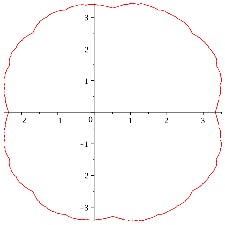
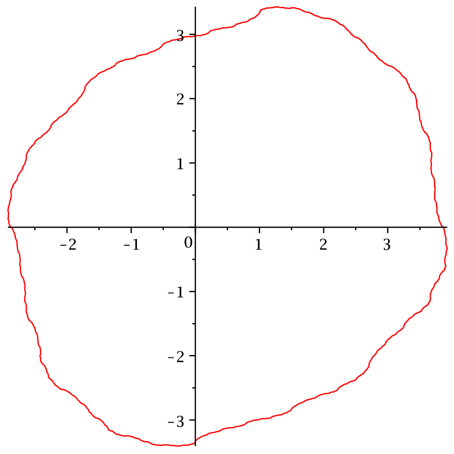
The effective lacunarity of the Fourier series makes calculations of the Julia set numerically effective if λ\lambda is not too large.

Refer to caption
Refer to caption
Figure 4. The Julia set of xn+1=λ​xn​(1−xn)x_{n+1}=\lambda x_{n}(1-x_{n}), for λ=0.3\lambda=0.3 and λ=0.3​i\lambda=0.3i, calculated from the Fourier series (30) discarding all o⁡(λ2)o(\lambda^{2}) terms. They coincide, within plot precision, with numerically calculated ones using standard iteration of maps algorithms.
Note 4.

  1. (i)

    Lacunarity of ψk\psi_{k} is a strong indication that ψ\psi has a natural boundary (in fact, it does have one), but not a proof. Transseriation at singular points and summation of convergent series (here in the parameter λ\lambda) do not commute. The transseries of HH on the barrier can be calculated by transasymptotic matching, see [6], but in this case is more simply found directly from the functional relation; see Note 7.

  2. (ii)

    In assessing the fine structure of the fractal using the Fourier expansion truncated to o⁡(λn)o(\lambda^{n}), the scale of analysis cannot evidently go below O⁡(λn)O(\lambda^{n}).

Remark 5.
  1. (i)

    For |λ||\lambda| sufficiently small, Theorem 6 provides a convenient way to determine the Julia set as well as the discrete evolution on the boundary.

  2. (ii)

    For small λ\lambda, the self similar structure is seen in

    ψ1​(ρ​exp⁡(2​π​i​m/2n))=∑k=1n−1ρ2j​exp⁡(2​π​i​m​2k−n)2j+ρ2n−22n−1​ψ1​(ρ)\psi_{1}(\rho\exp(2\pi im/2^{n}))=\sum_{k=1}^{n-1}\frac{\rho^{2^{j}}\exp(2\pi im2^{k-n})}{2^{j}}+\frac{\rho^{2^{n}-2}}{2^{n-1}}\psi_{1}(\rho)

    where the sum is a polynomial, thus analytic. Up to a scale factor of 2−n+12^{-n+1}, if |λ|≪2−n+1|\lambda|\ll 2^{-n+1}, the nontrivial structure of ψ\psi at exp⁡(2​π​i​m/2n)\exp(2\pi im/2^{n}) and at 11 are the same, see Note 4; that is

    ψ⁡(exp⁡(2​π​i​m/2n))=2−n+1​ψ​(1)+regular+o⁡(λ)\psi(\exp(2\pi im/2^{n}))={2^{-n+1}}\psi(1)+\text{regular}+o(\lambda)

    Exact transseries can be obtained for ψ\psi; see also Note 7.

  3. (iii)

    For iterations of the form xn+1=λk−1​Pk​(x)x_{n+1}=\lambda^{k-1}P_{k}(x) where PkP_{k} is a polynomial of degree k>2k>2, the calculations and the results, for small λ\lambda, are essentially the same. The lacunary series would involve the powers zkjz^{k^{j}}. For instance if the recurrence is xn+1=λ2​xn​(1−3​xn+xn2)x_{n+1}=\lambda^{2}x_{n}(1-3x_{n}+x_{n}^{2}), then ψ\psi is to be replaced by the solution of

    ψ=λ2​ψ∨3​(1+3​ψ+ψ2)\psi=\lambda^{2}\psi^{\vee 3}(1+3\psi+\psi^{2})

    and the small λ\lambda series will now have ψ1=∑k=1∞3−k−1​z3k\psi_{1}=\sum_{k=1}^{\infty}3^{-k-1}{{z^{3^{k}}}} and so on.

3. Proofs

Lemma 4.

Under the assumptions of Theorem 1, (iii), h​(y):=g−1​(y)h(y):=g^{-1}(y) also has a differentiable asymptotic power series as y→∞y\to\infty.

Proof.

Straightforward inversion of power series asymptotics, cf §5. ∎

3.1. Proof of Theorem 1

The proof of (4) (i) essentially amounts to showing that |f|2|f|^{2} is diagonally dominant, in that terms containing g⁡(j)g(j) and g⁡(k)g(k) with j≠kj\neq k are comparatively small, as shown in §3.8.

(ii) Since gg is increasing on (0,∞)(0,\infty), the result follows from the usual integral upper and lower bounds for a sum. Equation (7) follows from simple calculations, cf. §5.

3.2. Proof of Theorem 2

We prove part (ii); part (i) is similar, and simpler. By standard Fourier analysis we get

{u}=12−∑k=1∞sin⁡2​k​π​uk​π,u∉ℤ\{u\}=\frac{1}{2}-\sum_{k=1}^{\infty}\frac{\sin 2k\pi u}{k\pi},\ \ \ \ u\notin\mathbb{Z} (35)

where

‖{u}−12+∑k=1Msin⁡2​k​π​uk​π‖∞≤CM→Si​(π)​ as ​M→∞\left\|\{u\}-\frac{1}{2}+\sum_{k=1}^{M}\frac{\sin 2k\pi u}{k\pi}\right\|_{\infty}\leq C_{M}\to{\text{\rm Si}}(\pi)\text{ as }M\to\infty (36)

where Si is the sine integral, and Si(π\pi) is the constant in the Gibbs phenomenon. Let gmg_{m} be an analytic function such that g⁡(s)−gm​(s)=o⁡(s−m)g(s)-g_{m}(s)=o(s^{-m}) for large ss.

Lemma 5.

The analysis reduces to the case where hh is a finite sum of powers. Indeed,

f=e−x​g​(0)+∫0∞e−x​u​g−1​(u)​𝑑u+∫g⁡(0)∞e−x​u​{hm​(u)}​𝑑u+Rm−1​(x)f=e^{-xg(0)}+\int_{0}^{\infty}e^{-xu}g^{-1}(u)du+\int_{g(0)}^{\infty}e^{-xu}\{h_{m}(u)\}du+R_{m-1}(x) (37)

where Rm−1R_{m-1} is Cm−1C^{m-1} and hmh_{m} is a truncation of the asymptotic expansion of hh, such that h⁡(u)−hm​(u)=o⁡(u−m)h(u)-h_{m}(u)=o(u^{-m}).

Proof.

We have

∫0∞e−x​u​{h⁡(u)}​𝑑u=∑N=0∞∫g⁡(N)g⁡(N+1)e−x​u​(h⁡(u)−N)​𝑑u=∑N=0∞∫gm​(N)gm​(N+1)e−x​u​(hm​(u)−N)​du+Rm−1​(x)\int_{0}^{\infty}e^{-xu}\{h(u)\}du=\sum_{N=0}^{\infty}\int_{g(N)}^{g(N+1)}e^{-xu}(h(u)-N)du\\ =\sum_{N=0}^{\infty}\int_{g_{m}(N)}^{g_{m}(N+1)}e^{-xu}(h_{m}(u)-N)du+R_{m-1}(x) (38)

where

Rm−1(x)=∑N=0∞(∫g⁡(N)gm​(N)+∫gm​(N+1)g⁡(N+1))e−x​u{h(u)}du+∑N=0∞∫gm​(N)gm​(N+1)e−x​u(h(u)−hm(u))duR_{m-1}(x)=\sum_{N=0}^{\infty}\left(\int_{g(N)}^{g_{m}(N)}+\int_{g_{m}(N+1)}^{g(N+1)}\right)e^{-xu}\{h(u)\}du\\ +\sum_{N=0}^{\infty}\int_{g_{m}(N)}^{g_{m}(N+1)}e^{-xu}(h(u)-h_{m}(u))du (39)

Using (35) and (36) the proof follows and the fact that g⁡(N)−gm​(N)=o⁡(N−m)g(N)-g_{m}(N)=o(N^{-m}) and h⁡(u)−hm​(u)=o⁡(u−m)h(u)-h_{m}(u)=o(u^{-m}), the sum is rapidly convergent, and the result follows. ∎

Lemma 6.

If hh is a finite sum of powers, then f−e−x​g​(0)−∫0∞e−x​u​g−1​(u)​𝑑u∈C∞f-e^{-xg(0)}-\int_{0}^{\infty}e^{-xu}g^{-1}(u)du\in C^{\infty}.

Proof.

Using (35) and (36) we have

f1​(x)=x​∫0∞e−x​u​{hm​(u)}​𝑑u=12−∑k=1∞∫0∞e−x​u​sin⁡2​k​π​hm​(u)k​π​𝑑u=12−∑k=1∞12​k​π​i​∑σ=±1σ​∫0∞e−x​u+σ​2​k​π​i​hm​(u)​𝑑uf_{1}(x)=x\int_{0}^{\infty}e^{-xu}\{h_{m}(u)\}du=\frac{1}{2}-\sum_{k=1}^{\infty}\int_{0}^{\infty}e^{-xu}\frac{\sin 2k\pi h_{m}(u)}{k\pi}du\\ =\frac{1}{2}-\sum_{k=1}^{\infty}\frac{1}{2k\pi i}\sum_{\sigma=\pm 1}\sigma\int_{0}^{\infty}e^{-xu+\sigma 2k\pi ih_{m}(u)}du (40)

We deform the contours of integration along the directions σ​α\sigma\alpha respectively, say for α=π/2\alpha=\pi/2. The integral

f1=∫0i​∞un​e2​k​π​i​hm​(u)​𝑑uf_{1}=\int_{0}^{i\infty}u^{n}e^{2k\pi ih_{m}(u)}du (41)

exists for any nn and it is estimated by

|∫0i​∞un​e2​k​π​i​hm​(u)​𝑑u|<c​o​n​s​t.k−b⁡(n+1)​Γ​(n⁡(b+1))\left|\int_{0}^{i\infty}u^{n}e^{2k\pi ih_{m}(u)}du\right|<const.k^{-b(n+1)}\Gamma(n(b+1)) (42)

The termwise nth derivatives at 0+0^{+} of the series of f1​(x)f_{1}(x) converge rapidly, and the result follows. ∎

3.3. Proof of Theorem 3

Proof.

Let ϵ>0\epsilon>0 be arbitrary, let

SN=∑j=1Nei​y​g​(j);S0:=0S_{N}=\sum_{j=1}^{N}e^{iyg(j)};\ \ \ S_{0}:=0

and let N1N_{1} be large enough so that |SN/ρ⁡(N)−L|≤ϵ|S_{N}/\rho(N)-L|\leq\epsilon for N>N1N>N_{1}. Then, by looking at ei​ϕ​fe^{i\phi}f if necessary, we can assume that L≥0L\geq 0. We have

f⁡(x+i​y)=∑k=1∞e−x​g​(k)​(Sk−Sk−1)=∑k=1∞Skρ⁡(k)​(e−x​g​(k)−e−x​g​(k+1))​ρ​(k)=L⁡(y)​∑k=1∞(e−x​g​(k−1)−e−x​g​(k))​ρ​(k)+∑k=1∞(e−x​g​(k)−e−x​g​(k+1))​dk​ρ​(k)f(x+iy)=\sum_{k=1}^{\infty}e^{-xg(k)}(S_{k}-S_{k-1})=\sum_{k=1}^{\infty}\frac{S_{k}}{\rho(k)}(e^{-xg(k)}-e^{-xg(k+1)})\rho(k)\\ =L(y)\sum_{k=1}^{\infty}(e^{-xg(k-1)}-e^{-xg(k)}){\rho(k)}+\sum_{k=1}^{\infty}(e^{-xg(k)}-e^{-xg(k+1)})d_{k}{\rho(k)} (43)

where dk=L⁡(y)−Sk/ρ⁡(k)→0d_{k}=L(y)-S_{k}/\rho(k)\to 0 as k→∞k\to\infty. Now,

∑k=1∞e−x​g​(k)​(ρ⁡(k+1)−ρ⁡(k))∼∫0∞e−x​g​(k)​ρ′​(k)​𝑑k=:Φρ​(x).\sum_{k=1}^{\infty}e^{-xg(k)}(\rho(k+1)-\rho(k))\sim\int_{0}^{\infty}e^{-xg(k)}\rho^{\prime}(k)dk=:\Phi_{\rho}(x). (44)

and under the given assumptions Φρ→∞\Phi_{\rho}\to\infty as x→0x\to 0. Note that Φρ→∞\Phi_{\rho}\to\infty as x→0x\to 0 and the facts that e−x​g​(k)−e−x​g​(k+1)>0e^{-xg(k)}-e^{-xg(k+1)}>0, ρ⁡(k)>0\rho(k)>0 and dk→0d_{k}\to 0, readily imply that the last sum in (43) is o​(Φρ​(x))o(\Phi_{\rho}(x)); (12) is follows in a similar way. ∎

3.4. Proof of Theorem5

We rely on Theorem 3, and analyze the case b=3/2b=3/2; the case b∈ℕb\in\mathbb{N} is simpler. We have β=t/(2​π)\beta=t/(2\pi). Let Sˇj=∑k=1je−2​π​i​mn​k3.\check{S}_{j}=\sum\limits_{k=1}^{j}e^{-2\pi i\dfrac{m}{n}k^{3}}\!\!. It is clear that for m,n∈ℕm,n\in\mathbb{N} we have j−1​Sˇj→∑k=1ne−2​π​i​mn​k3=Lm​nj^{-1}\check{S}_{j}\to\sum\limits_{k=1}^{n}e^{-2\pi i\dfrac{m}{n}k^{3}}=L_{mn}. On the other hand, by summation by parts we get

SN=2​2​eπ​i/43​β​∑k=1kN−1k1/2​exp⁡(−8​π​i27​β2​k3)+O⁡(N1/4)=O⁡(N1/4)+2​2​eπ​i/43​β​(kN−1)3/2​SˇkN−1kN−1+2​2​eπ​i/43​β​∑k=1kN−1k−1​Sˇk​k​(k1/2−(k−1)1/2)S_{N}=\frac{2\sqrt{2}e^{\pi i/4}}{3\beta}\sum_{k=1}^{k_{N}-1}k^{1/2}\exp\left(-\frac{8\pi i}{27\beta^{2}}k^{3}\right)+O(N^{1/4})=O(N^{1/4})\\ +\frac{2\sqrt{2}e^{\pi i/4}}{3\beta}(k_{N}-1)^{3/2}\frac{\check{S}_{k_{N}-1}}{k_{N}-1}+\frac{2\sqrt{2}e^{\pi i/4}}{3\beta}\sum_{k=1}^{k_{N}-1}k^{-1}\check{S}_{k}k(k^{1/2}-(k-1)^{1/2}) (45)

and it is easy to check that, as N→∞N\to\infty we have

SN∼(2​2​eπ​i/43​β​(1+1/3))​kN3/2​Lm​n=8​2​eπ​i/49​β​3​β2​N3/4S_{N}\sim\left(\frac{2\sqrt{2}e^{\pi i/4}}{3\beta}(1+1/3)\right)k_{N}^{3/2}L_{mn}=\frac{8\sqrt{2}e^{\pi i/4}}{9\beta}\sqrt{\frac{3\beta}{2}}N^{3/4} (46)

where we used the definition of kNk_{N} following eq. (45), which implies kN∼32​N1/2​βk_{N}\sim\frac{3}{2}N^{1/2}\beta. The result follows by changes of variables, using (11) and noting that

34∫0∞e−x​k3/2k−1/4dk=π2​x\frac{3}{4}\int_{0}^{\infty}e^{-xk^{3/2}}k^{-1/4}dk=\frac{\sqrt{\pi}}{2\sqrt{x}} (47)

It is also clear that |j−1​Sˇj|≤1|j^{-1}\check{S}_{j}|\leq 1 and a similar calculation provides an overall upper bound.

Section 5.4 provides an independent way to calculate the behavior along the boundary.

3.5. Proof of Proposition 1

For b=2b=2 using (40) and ∫0∞e−p​xsin2kπp12dp=π3/2ke−k2​π2xx−3/2\int_{0}^{\infty}e^{-px}\sin 2k\pi p^{\frac{1}{2}}dp=\pi^{3/2}ke^{-\frac{k^{2}\pi^{2}}{x}}x^{-3/2} we immediately obtain

f⁡(x)=π2​x−12+πx​∑k=1∞e−k2​π2xf(x)=\frac{\sqrt{\pi}}{2\sqrt{x}}-\dfrac{1}{2}+\frac{\sqrt{\pi}}{\sqrt{x}}\sum_{k=1}^{\infty}e^{-\frac{k^{2}\pi^{2}}{x}}

3.6. The case g⁡(j)=ajg(j)=a^{j}

It is easy to see that, for this choice of gg, we have the functional relation

f⁡(z)−f⁡(a​z)=e−zf(z)-f(az)=e^{-z}

Since e−z→1e^{-z}\to 1 as z→0+z\rightarrow 0+, the leading behavior formally satisfies f⁡(z)−f⁡(a​z)∼1f(z)-f(az)\sim 1 i.e. f⁡(z)∼−log⁡zlog⁡af(z)\sim-\dfrac{\log z}{\log a}

In view of this we let f⁡(z)=−log⁡zlog⁡a+G⁡(z)f(z)=-\dfrac{\log z}{\log a}+G(z) which gives G⁡(z)−G⁡(a​z)=e−z−1G(z)-G(az)=e^{-z}-1 i.e.

G(z)=G(z/a)+(1−e−z/a)G(z)=G(z/a)+(1-e^{-z/a}) (48)

We first obtain a solution a solution Gˇ\check{G} of the homogeneous equation and then write G=Gˇ+h⁡(az)G=\check{G}+h(a^{z}), where hh now satisfies

h⁡(y)=h⁡(y+1){h}(y)={h}(y+1) (49)

Iterating (48) we obtain

Gˇ(z)=∑n=0∞(1−e−z/an)=−∑n=0∞∑k=1∞(−z)kk!​an​k=∑n=1∞(−z)nn!​(1−an)\check{G}(z)=\sum_{n=0}^{\infty}(1-e^{-z/a^{n}})=-\sum_{n=0}^{\infty}\sum_{k=1}^{\infty}\frac{(-z)^{k}}{k!a^{nk}}=\sum_{n=1}^{\infty}\frac{(-z)^{n}}{n!(1-a^{n})}

which is indeed an entire function and satisfies the functional relation. Now we return to (49). Since by its connection to f⁡(z)f(z), h{h} is obviously smooth in yy, it can be expressed in terms of its Fourier series

h⁡(y)=∑k=−∞∞ck​e2​k​π​i​y{h}(y)=\sum_{k=-\infty}^{\infty}c_{k}e^{2k\pi iy}

where the coefficients ck=c¯−kc_{k}=\bar{c}_{-k} can be found by using the original function ff. Recall that we have

f⁡(z)=−log⁡zlog⁡a+Gˇ​(z)+h⁡(log⁡zlog⁡a)f(z)=-\dfrac{\log z}{\log a}+\check{G}(z)+{h}\left(\dfrac{\log z}{\log a}\right)

which implies

h⁡(y)=f⁡(ay)+y−Gˇ​(ay){h}(y)=f(a^{y})+y-\check{G}(a^{y})
Lemma 7.

The Fourier coefficients of the periodic function h{h} are given by

ck=1log⁡a​Γ​(−2​k​π​ilog⁡a)​(k≠0)c_{k}=\frac{1}{\log a}\Gamma\left(-\frac{2k\pi i}{\log a}\right)\>\left(k\neq 0\right) (50)

and

c0=∫01f⁡(ay)​𝑑y+∫01y​𝑑y−∫01Gˇ​(ay)​𝑑yc_{0}=\int_{0}^{1}f(a^{y})dy+\int_{0}^{1}ydy-\int_{0}^{1}\check{G}(a^{y})dy

Since ck∼1π​log⁡a​e−|k|​π2log⁡ac_{k}\sim\sqrt{\dfrac{1}{\pi\log a}}e^{\frac{-|k|\pi^{2}}{\log a}}, (implying that the Fourier expansion for hh is valid exactly for Re⁡(z)>0\mathrm{Re}\left(z\right)>0) we have

f⁡(z)=−log⁡zlog⁡a+∑n=1∞(−z)nn!​(1−an)+c0+1log⁡a​∑k≠0Γ⁡(−2​k​π​ilog⁡a)​z2​k​π​ilog⁡af\left(z\right)=-\dfrac{\log z}{\log a}+\sum_{n=1}^{\infty}\frac{\left(-z\right)^{n}}{n!\left(1-a^{n}\right)}+c_{0}+\frac{1}{\log a}\sum_{k\neq 0}\Gamma\left(-\frac{2k\pi i}{\log a}\right)z^{\frac{2k\pi i}{\log a}}

The series further resums to

f⁡(z)=−log⁡zlog⁡a+∑n=1∞(−z)nn!​(1−an)+c0−z2​π​i​∫0∞logℝ⁡(−s2​π​ilog⁡a)​e−s​z​𝑑sf\left(z\right)=-\dfrac{\log z}{\log a}+\sum_{n=1}^{\infty}\frac{\left(-z\right)^{n}}{n!\left(1-a^{n}\right)}+c_{0}-\frac{z}{2\pi i}\int_{0}^{\infty}\log_{\mathbb{R}}\left(-s^{\frac{2\pi i}{\log a}}\right)e^{-sz}ds (51)

valid for z>0z>0.

The proof is given in §5.3.

Similar results hold for other rational angles if b∈ℕb\in\mathbb{N} (by grouping terms with the same phase). For example,

∑n=0∞e−2n​(z+25​π​i)=e−25​π​i​∑n=0∞e−24​n​z+e−45​π​i​∑n=0∞e−24​n+1​z+e−85​π​i​∑n=0∞e−24​n+2​z+e−65​π​i​∑n=0∞e−24​n+3​z=e−25​π​i​∑n=0∞e−16n​z+e−45​π​i​∑n=0∞e−16n​(2​z)+e−85​π​i​∑n=0∞e−16n​(4​z)+e−65​π​i​∑n=0∞e−16n​(8​z)\sum_{n=0}^{\infty}e^{-2^{n}(z+\frac{2}{5}\pi i)}\\ =e^{-\frac{2}{5}\pi i}\sum_{n=0}^{\infty}e^{-2^{4n}z}+e^{-\frac{4}{5}\pi i}\sum_{n=0}^{\infty}e^{-2^{4n+1}z}+e^{-\frac{8}{5}\pi i}\sum_{n=0}^{\infty}e^{-2^{4n+2}z}+e^{-\frac{6}{5}\pi i}\sum_{n=0}^{\infty}e^{-2^{4n+3}z}\\ =e^{-\frac{2}{5}\pi i}\sum_{n=0}^{\infty}e^{-16^{n}z}+e^{-\frac{4}{5}\pi i}\sum_{n=0}^{\infty}e^{-16^{n}(2z)}+e^{-\frac{8}{5}\pi i}\sum_{n=0}^{\infty}e^{-16^{n}(4z)}+e^{-\frac{6}{5}\pi i}\sum_{n=0}^{\infty}e^{-16^{n}(8z)} (52)

3.7. Proof of Theorem 4

(i) and (ii): By an argument similar to the one leading to (40) we have

f⁡(z)=∫0∞e−z​g​(s)​𝑑s−12+∑k=1∞12​k​π​i​∑σ=±1∫0σ​i​∞e−z​u+σ​2​k​π​i​u1/b​𝑑uf(z)=\int_{0}^{\infty}e^{-zg(s)}ds-\frac{1}{2}+\sum_{k=1}^{\infty}\frac{1}{2k\pi i}\sum_{\sigma=\pm 1}\int_{0}^{\sigma i\infty}e^{-zu+\sigma 2k\pi iu^{1/b}}du (53)

The exponential term ensures convergence in kk. Taking sb=ts^{b}=t we see that

∫0∞e−z​sbdp=Γ(1+1/b)z−1/b\int_{0}^{\infty}e^{-zs^{b}}dp=\Gamma(1+1/b)z^{-1/b} (54)

We now analyze the case σ=−1\sigma=-1, the other case being similar. A term in the sum is

12​k​π​i​∫0i​∞e−z​u−2​k​π​i​u1/b​𝑑u=(kz)d​∫0∞e−νk​(t+2​π​i​t1/b)​𝑑t=(kz)d∫0∞e−νk​sHˇ−(s)ds=z−d∫0∞e−z−1/(b−1)sHˇ−(s/kd)ds\frac{1}{2k\pi i}\int_{0}^{i\infty}e^{-zu-2k\pi iu^{1/b}}du=\left(\frac{k}{z}\right)^{{d}}\int_{0}^{\infty}e^{-\nu_{k}(t+2\pi it^{1/b})}dt\\ =\left(\frac{k}{z}\right)^{{d}}\int_{0}^{\infty}e^{-\nu_{k}s}{\check{H}_{-}}(s)ds=z^{-{d}}\int_{0}^{\infty}e^{-z^{-1/(b-1)}s}{\check{H}_{-}}(s/k^{{d}})ds (55)

where νk=kdz−1/(b−1)\nu_{k}={k^{{d}}}{z^{-1/(b-1)}}, Hˇ−​(s)=ϕ′​(s){\check{H}_{-}}(s)=\phi^{\prime}(s) and

Φ⁡(ϕ⁡(u)):=ϕ⁡(u)+2​π​i​ϕ​(u)1/b=u\Phi(\phi(u)):=\phi(u)+2\pi i\phi(u)^{1/b}=u (56)

(a) Near the origin, we write ϕ=ub​Hb\phi=u^{b}H_{b}, and we get

Hb=12​π​i​(1−ub−1​Hb)bH_{b}=\frac{1}{2\pi i}(1-u^{b-1}H_{b})^{b}

and analyticity of HbH_{b} in ub−1u^{b-1} follows, for instance, from the contractive mapping principle.

(b) The only singularities of ϕ\phi, thus of Hˇ−{\check{H}_{-}}, are the points implicitly given by Φ′=0\Phi^{\prime}=0.

(b) It is also easy to check that for some C>0C>0 we have

|Hˇ−​(u)|≤C​|ub−1|1+|ub−1||{\check{H}_{-}}(u)|\leq C\frac{|u^{b-1}|}{1+|u^{b-1}|} (57)

uniformly in ℂ\mathbb{C}, with a cut at the singularity, or on a corresponding Riemann surface. From (57) we see that the sum

H−=∑k=1∞Hˇ−​(s/kq)H_{-}=\sum_{k=1}^{\infty}{\check{H}_{-}}(s/k^{{q}}) (58)

converges, on compact sets in ss, at least as fast as c​o​n​s​t​∑k−bconst\sum k^{-b}, thus it is an analytic function wherever all Hˇ−​(s/kd){\check{H}_{-}}(s/k^{{d}}) are analytic, that is, in ℂ\mathbb{C} except for the points kd​s0k^{d}s_{0}. Using an integral estimate, we get the global bound

|H−|≤c​o​n​s​t​∑k=1∞|u|b−1kq+|u|b−1≤c​o​n​s​t​|u|(b−1)2/b|H_{-}|\leq const\sum_{k=1}^{\infty}\frac{|u|^{b-1}}{k^{q}+|u|^{b-1}}\leq const|u|^{(b-1)^{2}/b} (59)

as |u|→∞|u|\to\infty.

The function HH in the lemma is simply H−+H−H_{-}+H_{-} where H+H_{+} is obtained from H−H_{-} by replacing ii by −i-i. The calculation of the explicit power series is straightforward, from (56), (58) and the similar formulae for H+H_{+}, using dominated convergence based on (59). We provide the details for convenience.

We write the last term in (55) in the form

fk​(z)=(kz)bb−1​∫Ce−s​(kbz)1b−1​Hˇ−​𝑑sf_{k}(z)=\left(\frac{k}{z}\right)^{\frac{b}{b-1}}\intop_{C}e^{-s(\frac{k^{b}}{z})^{\frac{1}{b-1}}}\check{H}_{-}ds (60)

where the contour CC is a curve from the origin to ∞\infty in the first quadrant.

Watson’s lemma implies

fk​(z)=∑j=1Nbj​k−j​b​zj−1+RN​(k,z)f_{k}(z)=\sum_{j=1}^{N}b_{j}k^{-jb}z^{j-1}+R_{N}(k,z)

where bjb_{j}can be calculated explicitly from Lagrange-Bürmann inversion formula used for the inverse function ϕ−1\phi^{-1} and RN​(k,z)≦C​k−(N+1)​b​zNR_{N}(k,z)\leqq Ck^{-(N+1)b}z^{N}, for arbitrary N∈ℕN\in\mathbb{N}. It follows that

f⁡(z)∼Γ⁡(1+1b)​z−1b−12+i2​π​∑j=1∞(1−(−1)j​b)​ζ​(j​b+1)​bj​zjf(z)\sim\Gamma(1+\dfrac{1}{b})z^{-\frac{1}{b}}-\dfrac{1}{2}+\frac{i}{2\pi}\sum_{j=1}^{\infty}(1-(-1)^{jb})\zeta(jb+1)b_{j}z^{j} (61)

which holds for z→0z\rightarrow 0 in the right half plane in any direction not tangential to the imaginary axis.

(iii) We obtain the transseries (which gives us information near the imaginary axis) by using the global properties of Hˇ−\check{H}_{-}, and standard deformation of the Laplace contour.

As zz goes around the complex plane, as usual in Laplace-like integrals, we rotate ss in (83) simultaneously, to keep the exponent real and positive. In the process, as we cross singularities, we collect a contribution to the integral from the point s−s_{-} above; the contribution is an integral around a cut originating at s−s_{-}. The singularity is integrable, and collapsing the contour to the cut itself, we get a contribution again in the form of a Laplace transform. This is the Borel sum (in the same variable, z−1/(b−1)z^{-1/(b-1)}.

Generically s−s_{-} is a square root branch point and we have

d​s−d​s=∑j=0∞c~j​[s−(b​i2​π)b1−b]j−12\frac{ds_{-}}{ds}=\sum_{j=0}^{\infty}\tilde{c}_{j}\left[s-\left(\dfrac{bi}{2\pi}\right)^{\frac{b}{1-b}}\right]^{\frac{j-1}{2}}

The asymptotic expansion of the cut contribution, Borel summable as we mentioned, is

exp⁡(−(2​π)bb−1​(bb1−b−b11−b)​ib1−b​(kbz)1b−1)​∑j=0∞cj​(zkb)2​j+12​(b−1)\exp\left({-(2\pi)^{\frac{b}{b-1}}(b^{\frac{b}{1-b}}-b^{\frac{1}{1-b}})i^{\frac{b}{1-b}}\left(\frac{k^{b}}{z}\right)^{\frac{1}{b-1}}}\right)\sum_{j=0}^{\infty}c_{j}\left(\frac{z}{k^{b}}\right)^{\frac{2j+1}{2(b-1)}}

The exponential term ensures convergence in kk of the Borel summed transseries. A similar result can be obtained for −k.-k.

Thus, the transseries of ff is of the form

f~​(z)=Γ⁡(1+1b)​z−1b−12+i2​π​∑j=1∞(1−(−1)j​b)​ζ​(j​b+1)​bj​zj\tilde{f}(z)=\Gamma(1+\dfrac{1}{b})z^{-\frac{1}{b}}-\dfrac{1}{2}+\frac{i}{2\pi}\sum_{j=1}^{\infty}(1-(-1)^{jb})\zeta(jb+1)b_{j}z^{j}
+{i2​π​∑k=1∞e(b−1)​(2​πb​i)bb−1​(kbz)1b−1​∑j=0∞cj​k−2​j​b+2−b2​(b−1)​z2​j−12​(b−1)−π2⩽arg⁡z⩽θ1−i2​π∑k=1∞e(b−1)​(2​πb​i)bb−1​((−k)bz)1b−1∑j=0∞cj(−k)−2​j​b+2−b2​(b−1)z2​j−12​(b−1)θ2⩽arg⁡z⩽π2+\begin{cases}\frac{i}{2\pi}\sum\limits_{k=1}^{\infty}e^{(b-1)(\frac{2\pi}{bi})^{\frac{b}{b-1}}(\frac{k^{b}}{z})^{\frac{1}{b-1}}}\sum\limits_{j=0}^{\infty}c_{j}k^{\frac{-2jb+2-b}{2(b-1)}}z^{\frac{2j-1}{2(b-1)}}&\,-\frac{\pi}{2}\leqslant\arg z\leqslant\theta_{1}\\ -\frac{i}{2\pi}\sum\limits_{k=1}^{\infty}e^{(b-1)(\frac{2\pi}{bi})^{\frac{b}{b-1}}(\frac{(-k)^{b}}{z})^{\frac{1}{b-1}}}\sum\limits_{j=0}^{\infty}c_{j}(-k)^{\frac{-2jb+2-b}{2(b-1)}}z^{\frac{2j-1}{2(b-1)}}&\,\theta_{2}\leqslant\arg z\leqslant\frac{\pi}{2}\end{cases}
Remark 6.

The analysis can be extended to the case

f⁡(z)=∑k=1∞F⁡(k)​e−kb​z​(λ≠0)f(z)=\sum_{k=1}^{\infty}F(k)e^{-k^{b}z}\>(\lambda\neq 0)

by noticing that

f⁡(z)=∫0∞(z​F​(p)−F′​(p))​e−p​z​[p1b]​𝑑pf(z)=\int_{0}^{\infty}(zF(p)-F^{\prime}(p))e^{-pz}[p^{\frac{1}{b}}]dp

If the expression of F⁡(k)F(k) is simple, for example F⁡(k)F(k) is a finite combination of terms of the form μk1b​kλ​(log⁡k)m​(m=0,1,2,3​…)\mu^{k^{\frac{1}{b}}}k^{\lambda}(\log k)^{m}\>(m=0,1,2,3...), the method in this section applies with little change to calculate the transseries of f⁡(z)f(z).

For special values of bb, asymptotic information as zz approaches the imaginary line can be obtained in the following way. Let z=δ+2​π​i​βz=\delta+2\pi i\beta and

f⁡(z)=∑k=1∞e−kb​(δ+2​π​i​β)​(Re⁡(δ)>0)f(z)=\sum_{k=1}^{\infty}e^{-k^{b}(\delta+2\pi i\beta)}\>(\mathrm{Re}(\delta)>0)

If 1<b∈ℕ1<b\in\mathbb{N}, we may obtain the asymptotic behavior for all rational β=mn\beta=\dfrac{m}{n}, by noting that e−kb​(2​π​i​β)=e−(k+n)b​(2​π​i​β)e^{-k^{b}(2\pi i\beta)}=e^{-(k+n)^{b}(2\pi i\beta)} and splitting the sum into

f⁡(z)=∑j=0∞∑l=1ne−(n​j+l)b​(δ+2​π​i​mn)=∑l=1ne−2​π​i​mn​lb​∑j=0∞e−(n​j+l)b​δf(z)=\sum_{j=0}^{\infty}\sum_{l=1}^{n}e^{-(nj+l)^{b}\left(\delta+2\pi i\dfrac{m}{n}\right)}=\sum_{l=1}^{n}e^{-2\pi i\dfrac{m}{n}l^{b}}\sum_{j=0}^{\infty}e^{-(nj+l)^{b}\delta}

It follows that

∑j=0∞e−(n​j+l)b​δ=nb​δ​∫lb/nb∞e−nb​δ​s​(s1b−l/n)​𝑑s\sum_{j=0}^{\infty}e^{-(nj+l)^{b}\delta}=n^{b}\delta\int_{l^{b}/n^{b}}^{\infty}e^{-n^{b}\delta s}\left(s^{\frac{1}{b}}-l/n\right)ds
=nb​δ​∫lb/nb∞e−nb​δ​s​(s1b−l/n)​𝑑s−nb​δ​∫lb/nb∞e−nb​δ​s​{s1b−l/n}​𝑑s=n^{b}\delta\int_{l^{b}/n^{b}}^{\infty}e^{-n^{b}\delta s}\left(s^{\frac{1}{b}}-l/n\right)ds-n^{b}\delta\int_{l^{b}/n^{b}}^{\infty}e^{-n^{b}\delta s}\left\{s^{\frac{1}{b}}-l/n\right\}ds

by the argument above. Since the absolute value of the fractional part does not exceed one, we have the estimate

∑j=0∞e−(n​j+l)b​δ=nb​δ​∫(ln)b∞e−nb​δ​s​s1b​𝑑s+O⁡(1)=1n​Γ​(1+1b)​δ−1b+O⁡(1)​(z→0)\sum_{j=0}^{\infty}e^{-(nj+l)^{b}\delta}=n^{b}\delta\int_{(\frac{l}{n})^{b}}^{\infty}e^{-n^{b}\delta s}s^{\frac{1}{b}}ds+O(1)=\frac{1}{n}{\Gamma\left(1+\dfrac{1}{b}\right)}\delta^{-\frac{1}{b}}+O(1)\>(z\rightarrow 0)

This implies

f⁡(z)=1n​∑l=1ne−2​π​i​mn​lb​Γ​(1+1b)​z−1b+O⁡(1)f(z)=\frac{1}{n}\sum_{l=1}^{n}e^{-2\pi i\dfrac{m}{n}l^{b}}\Gamma\left(1+\dfrac{1}{b}\right)z^{-\frac{1}{b}}+O(1) (62)

Therefore f⁡(z)f(z) either blows up like z−1bz^{-\frac{1}{b}}(when ∑l=1ne−2​π​i​mn​lb≠0\sum_{l=1}^{n}e^{-2\pi i\dfrac{m}{n}l^{b}}\neq 0) or it is bounded (when ∑l=1ne−2​π​i​mn​lb=0\sum_{l=1}^{n}e^{-2\pi i\dfrac{m}{n}l^{b}}=0).

The Fourier expansion of the fractional part can be used to calculate the transseries as we did for β=0\beta=0, but we shall omit the calculation here.

For special values of bb, asymptotic information is relatively easy to obtain on a dense set along the barrier. This is the case when b=r+1rb=\dfrac{r+1}{r} where r∈ℕr\in\mathbb{N}; then, the transseries contains exponential sums in terms of integer powers, krk^{r}, a consequence of the duality relation 1b+1d=1\dfrac{1}{b}+\dfrac{1}{d}=1, which at the transseries level is of the form ∑e−kb​z→g1+∑eckdz−d/bg2\sum e^{-k^{b}z}\rightarrow g_{1}+\sum e^{ck^{d}z^{-d/b}}g_{2} where g1,g2g_{1},g_{2} are power series. We illustrate this for b=32b=\dfrac{3}{2}.

Without loss of generality, we assume β<0\beta<0. The transseries of ff is given in (87). To estimate the asymptotic behavior of f⁡(z)f(z) as zz approaches the imaginary line, we rewrite (87) as

f⁡(z)=Γ⁡(53)​z−23−12+i2​π∑k=1∞(kz)2∫0∞e−s​k3z2(34​2​(π​i)32s12−3​i8​π3s−105​i32256​2​π92s32+⋯)ds+∑k=1∞e32​i​π3​k327​z24​2​i−12​π3k12z−1iπ​∑k=1∞(kz)2​e−32​i​π3​k327​z2​∫0∞e−s​k3z2​(i−128​2​π34​(s−s0)12+⋯)​𝑑sf(z)=\Gamma\left(\frac{5}{3}\right)z^{-\frac{2}{3}}-\dfrac{1}{2}\\ +\frac{i}{2\pi}\sum_{k=1}^{\infty}\left(\frac{k}{z}\right)^{2}\int_{0}^{\infty}e^{-s\frac{k^{3}}{z^{2}}}\left(\dfrac{3}{4\sqrt{2}(\pi i)^{\frac{3}{2}}}s^{\frac{1}{2}}-\dfrac{3i}{8\pi^{3}}s-\dfrac{105i^{\frac{3}{2}}}{256\sqrt{2}\pi^{\frac{9}{2}}}s^{\frac{3}{2}}+\cdots\right)ds\\ +\sum_{k=1}^{\infty}e^{\dfrac{32i\pi^{3}k^{3}}{27z^{2}}}\dfrac{4\sqrt{2}i^{-\frac{1}{2}}\pi}{3}k^{\frac{1}{2}}z^{-1}\\ \frac{i}{\pi}\sum_{k=1}^{\infty}\left(\frac{k}{z}\right)^{2}e^{-\dfrac{32i\pi^{3}k^{3}}{27z^{2}}}\int_{0}^{\infty}e^{-s\frac{k^{3}}{z^{2}}}\left(\dfrac{i^{-\frac{1}{2}}}{8\sqrt{2}\pi^{\frac{3}{4}}}(s-s_{0})^{\frac{1}{2}}+\cdots\right)ds (63)

Watson’s Lemma implies that

f⁡(z)=4​2​i−12​π3​z​∑k=1∞k12​e32​i​π3​k327​z2+O⁡(1)f(z)=\dfrac{4\sqrt{2}i^{-\frac{1}{2}}\pi}{3z}\sum_{k=1}^{\infty}k^{\frac{1}{2}}e^{\dfrac{32i\pi^{3}k^{3}}{27z^{2}}}+O(1) (64)

The is sum in (64) is similar to the sum with b=3b=3, and can be estimated in a similar way:

∑k=1∞k12​e−(y+2​π​i​mn)=(∑l=1ne−2​π​i​mn​l3)​π3​n​y+o⁡(1y)\sum_{k=1}^{\infty}k^{\frac{1}{2}}e^{-(y+2\pi i\frac{m}{n})}=\left(\sum_{l=1}^{n}e^{-2\pi i\dfrac{m}{n}l^{3}}\right)\frac{\sqrt{\pi}}{3n\sqrt{y}}+o\left(\frac{1}{\sqrt{y}}\right)

Setting 32​i​π3​k327​z2=y+2​π​i​mn\dfrac{32i\pi^{3}k^{3}}{27z^{2}}=y+2\pi i\dfrac{m}{n} , we have z=−4​π​i3​3​nmz=-\dfrac{4\pi i}{3\sqrt{3}}\sqrt{\dfrac{n}{m}}+(nm)32​y+o⁡(y)\left(\dfrac{n}{m}\right)^{\frac{3}{2}}y+o(y). The asymptotic behavior can be obtained for β=−4​π​i3​3​nm\beta=-\dfrac{4\pi i}{3\sqrt{3}}\sqrt{\dfrac{n}{m}} (this includes all rationals) by substituting y=32​i​π3​k327​z2−2​π​i​mny=\dfrac{32i\pi^{3}k^{3}}{27z^{2}}-2\pi i\dfrac{m}{n} in the above estimates. Setting z=−4​π​i3​3​nmz=-\dfrac{4\pi i}{3\sqrt{3}}\sqrt{\dfrac{n}{m}}+δ\delta (δ>0\delta>0), a direct calculation shows that

Re⁡(z)​f​(z)=6​π​i374​(nm)14​1n​∑l=1ne−2​π​i​mn​l3+o⁡(1)\sqrt{\mathrm{Re}(z)}f(z)=\frac{\sqrt{6\pi i}}{3^{\frac{7}{4}}}\left(\frac{n}{m}\right)^{\frac{1}{4}}\frac{1}{n}\sum_{l=1}^{n}e^{-2\pi i\dfrac{m}{n}l^{3}}+o(1) (65)

3.8. Details of the proof of Theorem 1

Consider, more generally,

f⁡(δ,β)=∑k=0∞a⁡(k)​e−g​(k)​(δ+2​π​i​β),δ>0f(\delta,\beta)=\sum_{k=0}^{\infty}a(k)e^{-g(k)(\delta+2\pi i\beta)}\>,\ \ \delta>0

where g⁡(k)>0g(k)>0 is a real function and∫0∞|a⁡(t)|2​𝑑t=∞\int_{0}^{\infty}|a(t)|^{2}dt=\infty.

We find the behavior of

∫β0β1|f⁡(δ,β)|2​𝑑β=∫β0β1∑k=0∞|a⁡(k)|2​e−2​g​(k)​δ​𝑑β+∫β0β1∑k≠ja⁡(k)​a¯​(j)​e−(g⁡(k)+g⁡(j))​δ+(g⁡(j)−g⁡(k))​2​π​i​β​𝑑β=(β1−β0)​∑k=0∞|a⁡(k)|2​e−2​g​(k)​δ+12​π​i∑k≠ja⁡(k)​a¯​(j)g⁡(j)−g⁡(k)e−(g⁡(k)+g⁡(j))​δe(g⁡(j)−g⁡(k))​2​π​i​β0(e(g⁡(j)−g⁡(k))​2​π​i​(β1−β0)−1)\int_{\beta_{0}}^{\beta_{1}}|f(\delta,\beta)|^{2}d\beta\\ =\int_{\beta_{0}}^{\beta_{1}}\sum_{k=0}^{\infty}|a(k)|^{2}e^{-2g(k)\delta}d\beta+\int_{\beta_{0}}^{\beta_{1}}\sum_{k\neq j}a(k)\bar{a}(j)e^{-(g(k)+g(j))\delta+(g(j)-g(k))2\pi i\beta}d\beta\\ =(\beta_{1}-\beta_{0})\sum_{k=0}^{\infty}|a(k)|^{2}e^{-2g(k)\delta}\\ +\frac{1}{2\pi i}\sum_{k\neq j}\frac{a(k)\bar{a}(j)}{g(j)-g(k)}e^{-(g(k)+g(j))\delta}e^{(g(j)-g(k))2\pi i\beta_{0}}\left(e^{(g(j)-g(k))2\pi i(\beta_{1}-\beta_{0})}-1\right) (66)

where β0,1∈ℝ\beta_{0,1}\in\mathbb{R} are arbitrary, or after mm integrations,

F(δ)=∫βm−1βm−1+cm−1⋯∫β1β1+c1∫β0β0+c0|f(δ,β)|2dβdβ0⋯dβm−2=c0c1⋯cm∑k=0∞|a(k)|2e−2​g​(k)​δ+O(∑k≠j|a⁡(k)​a¯​(j)(g⁡(j)−g⁡(k))m|e−(g⁡(k)+g⁡(j))​δ)F(\delta)=\int_{\beta_{m-1}}^{\beta_{m-1}+c_{m-1}}\cdots\int_{\beta_{1}}^{\beta_{1}+c_{1}}\int_{\beta_{0}}^{\beta_{0}+c_{0}}|f(\delta,\beta)|^{2}d\beta d\beta_{0}\cdots d\beta_{m-2}\\ =c_{0}c_{1}\cdots c_{m}\sum_{k=0}^{\infty}|a(k)|^{2}e^{-2g(k)\delta}+O\left(\sum_{k\neq j}\left|\frac{a(k)\bar{a}(j)}{(g(j)-g(k))^{m}}\right|e^{-(g(k)+g(j))\delta}\right) (67)

Note that

∑k≠j|a⁡(k)​a¯​(j)(g⁡(j)−g⁡(k))m|​e−(g⁡(k)+g⁡(j))​δ=2​∑k=0∞∑n=1∞|a⁡(k)​a¯​(k+n)(g⁡(k+n)−g⁡(k))m|​e−(g⁡(k)+g⁡(k+n))​δ=2​∑k=0∞|a⁡(k)|​e−2​g​(k)​δ​∑n=1∞|a⁡(k+n)(g⁡(k+n)−g⁡(k))m|​e−(g⁡(k+n)−g⁡(k))​δ=O⁡(∑k=0∞|a⁡(k)|​e−2​g​(k)​δ​∑n=1∞|a⁡(k+n)(g⁡(k+n)−g⁡(k))m|)\sum_{k\neq j}\left|\frac{a(k)\bar{a}(j)}{(g(j)-g(k))^{m}}\right|e^{-(g(k)+g(j))\delta}\\ =2\sum_{k=0}^{\infty}\sum_{n=1}^{\infty}\left|\frac{a(k)\bar{a}(k+n)}{(g(k+n)-g(k))^{m}}\right|e^{-(g(k)+g(k+n))\delta}\\ =2\sum_{k=0}^{\infty}|a(k)|e^{-2g(k)\delta}\sum_{n=1}^{\infty}\left|\frac{a(k+n)}{(g(k+n)-g(k))^{m}}\right|e^{-(g(k+n)-g(k))\delta}\\ =O\left(\sum_{k=0}^{\infty}|a(k)|e^{-2g(k)\delta}\sum_{n=1}^{\infty}\left|\frac{a(k+n)}{(g(k+n)-g(k))^{m}}\right|\right) (68)

under our assumption.

If furthermore we have

∑n=1∞|a⁡(k+n)(g⁡(k+n)−g⁡(k))m|=o⁡(a⁡(k))\sum_{n=1}^{\infty}\left|\frac{a(k+n)}{(g(k+n)-g(k))^{m}}\right|=o(a(k))

then we obtain

F(δ)=c0c1⋯cm∑k=0∞|a(k)|2e−2​g​(k)​δ+O(∑k=0∞|a⁡(k)|2G⁡(k)e−2​g​(k)​δ)F(\delta)=c_{0}c_{1}\cdots c_{m}\sum_{k=0}^{\infty}|a(k)|^{2}e^{-2g(k)\delta}+O\left(\sum_{k=0}^{\infty}\frac{|a(k)|^{2}}{G(k)}e^{-2g(k)\delta}\right) (69)

where G⁡(k)>1,G⁡(k)→∞G(k)>1,\,G(k)\rightarrow\infty as k→∞k\rightarrow\infty, or

F(δ)(∑k=0∞|a(k)|2e−2​g​(k)​δ)−1=c0⋯cm+o(1)asδ→0+F(\delta)\left(\sum_{k=0}^{\infty}|a(k)|^{2}e^{-2g(k)\delta}\right)^{-1}=c_{0}\cdots c_{m}+o(1)\ \ as\ \delta\to 0^{+} (70)

The result now follows from the following lemma.

Proposition 8.

Assume

(i) hn:ℝ→[0,∞)h_{n}:\mathbb{R}\to[0,\infty) are locally L1L^{1}, and

(ii) limn→∞∫Bhn(x1+⋯+xN)dx1⋯dxN=meas(B)\displaystyle\lim_{n\to\infty}\int_{B}h_{n}(x_{1}+\cdots+x_{N})dx_{1}\cdots dx_{N}=meas(B) for any box B=∏i=1N[ai,bi]B\displaystyle=\prod_{i=1}^{N}[a_{i},b_{i}].

Then hn→1h_{n}\to 1 in the dual of C⁡[α,β]C[\alpha,\beta] for any [α,β][\alpha,\beta].

Proof.

We first take N=2N=2, the general case will follow by induction on NN.

Consider the rectangle Bc=(a,b−c)×(0,c)B_{c}=(a,b-c)\times(0,c), 0<c<b−a0<c<b-a. By changing coordinates to x+y=s,y=y′x+y=s,y=y^{\prime}, we get that

c−1​∫Bhn​𝑑y​𝑑x=∫abhn​(s)​Ta,b;c​(s)​𝑑s→m​e​a​s​(Ta,b;c);as ​n→∞c^{-1}\int_{B}h_{n}dydx=\int_{a}^{b}h_{n}(s)T_{a,b;c}(s)ds\to meas(T_{a,b;c});\ \text{as }n\to\infty (71)

where Ta,b;c​(⋅)T_{a,b;c}(\cdot) is the function having Ta,b;cT_{a,b;c} as a graph, Ta,b;cT_{a,b;c} being an isosceles trapezoid with lower base the interval (a,b)(a,b) and upper base of length b−a−2​cb-a-2c at height 1.

We also note that the indicator function of [a,b][a,b], 𝟏a​b\mathbf{1}_{ab}, satisfies the inequalities Ta−c,b+c;c≥𝟏a​b≥Ta,b;cT_{a-c,b+c;c}\geq\mathbf{1}_{ab}\geq T_{a,b;c}. Thus, since cc is arbitrary and hn≥0h_{n}\geq 0, and both m​e​a​s​(Ta−c,b+c;c)meas(T_{a-c,b+c;c}), and m​e​a​s​(Ta,b;c)meas(T_{a,b;c}) tend to (b−a)(b-a) as c→0c\to 0, we have

limn→∞∫abhn​(s)​𝑑s=(b−a)=m​e​a​s​([a,b])\lim_{n\to\infty}\int_{a}^{b}h_{n}(s)ds=(b-a)=meas([a,b]) (72)

In particular, given α<β\alpha<\beta, ‖hn‖L1​[α,β]\|h_{n}\|_{L^{1}[\alpha,\beta]} are uniformly bounded, that is, for some C≥1C\geq 1 we have

supn≥1‖hn‖L1​[α,β]≤C⁡(β−α)\sup_{n\geq 1}\|h_{n}\|_{L^{1}[\alpha,\beta]}\leq C(\beta-\alpha) (73)

Since a continuous function on [α,β][\alpha,\beta] is approximated arbitrarily well in sup norm by finite linear combinations of indicator functions of intervals, it follows from (72), (73) 66 6 Alternatively, and somewhat more compactly, one can prove the result without the intermediate steps (72) and (73) by upper and lower bounding continuous functions by sums of trapezoids. and the triangle inequality that

∫αβhn​(s)​f​(s)​𝑑s→∫αβf⁡(s)​𝑑s,∀f∈C⁡[α,β]\int_{\alpha}^{\beta}h_{n}(s)f(s)ds\to\int_{\alpha}^{\beta}f(s)ds,\ \forall\,f\in C[\alpha,\beta] (74)

For general NN we use hn−(s)=∫B′hn(s+x1+…+xN−1)dx1⋯dxN−1h^{-}_{n}(s)=\int_{B^{\prime}}h_{n}(s+x_{1}+...+x_{N-1})dx_{1}\cdots dx_{N-1} and (72) to reduce the problem to N−1N-1. ∎

The condition

∑n=1∞|a⁡(k+n)(g⁡(k+n)−g⁡(k))m|=o⁡(a⁡(k))\sum_{n=1}^{\infty}\left|\frac{a(k+n)}{(g(k+n)-g(k))^{m}}\right|=o(a(k))

is satisfied, for instance, if

(1) ∃c>0\exists c>0 so that c<|a⁡(k)|<c−1c<|a(k)|<c^{-1}, or |a⁡(k)||a(k)| decreases to 0. (Note that g⁡(k+n)−g⁡(k)=g′​(k+t​n)​ng(k+n)-g(k)=g^{\prime}(k+tn)n, where 0⩽t⩽10\leqslant t\leqslant 1, and g′​(k)→∞g^{\prime}(k)\rightarrow\infty as k→∞k\rightarrow\infty.)

(2) ∃c,r\exists c,r so that c<a⁡(k)<krc<a(k)<k^{r}. g′​(k)⩾kεg^{\prime}(k)\geqslant k^{\varepsilon} for some small ε>0\varepsilon>0.

4. Proof of Theorem 6

In Appendix §5.5 we list some known facts about iterations of maps.

Proof of Bötcher’s theorem, for (28).

(Note: this line of proof extends to general analytic maps.)

We write ψ=λ​z+λ2​z​g​(z)\psi=\lambda z+\lambda^{2}zg(z) and obtain

g⁡(z)−12​g​(z2)=12​z+12​λ​[g⁡(z)​(z−g⁡(z))+g⁡(z2)]+λ2​z2​g​(z)​g​(z2)=N⁡(g)g(z)-\frac{1}{2}g(z^{2})=\frac{1}{2}z+\frac{1}{2}\lambda\left[g(z)(z-g(z))+g(z^{2})\right]+\frac{\lambda^{2}z}{2}g(z)g(z^{2})=N(g) (75)

Let 𝒜λ\mathcal{A_{\lambda}} denote the functions analytic in the polydisk ℙ1,ϵ=𝔻×{λ:|λ|<ϵ}\mathbb{P}_{1,\epsilon}=\mathbb{D}\times\{\lambda:|\lambda|<\epsilon\}. We write (75) in the form (see 29))

g=2​𝔗​N​(g)g=2\mathfrak{T}N(g) (76)

This equation is manifestly contractive in the sup norm, in a ball of radius slightly larger than 1/21/2 in 𝒜λ\mathcal{A_{\lambda}}, if ϵ\epsilon is small enough. For λ≠0\lambda\neq 0, evidently ψ=ϕ−1\psi=\phi^{-1} is also analytic at zero. ∎

Lemma 9.

ψ\psi is analytic in 𝔻1\mathbb{D}_{1} for all λ\lambda with |λ|<1|\lambda|<1.

Proof.

We have

ψ⁡(z)=λ2​(X+X2+4​X/λ)=:F⁡(X);X=ψ⁡(z2)\psi(z)=\frac{\lambda}{2}\left(X+\sqrt{X^{2}+4X/\lambda}\right)=:F(X);\ X=\psi(z^{2}) (77)

For small z≠0z\neq 0, ψ⁡(z)=O⁡(z)\psi(z)=O(z) and thus F⁡(ψ⁡(z2))F(\psi(z^{2})) is well defined and analytic. Note that (77) provides analytic continuation of ψ\psi from 𝔻ρ2\mathbb{D}_{\rho^{2}} to 𝔻ρ\mathbb{D}_{{\rho}}, provided nowhere in 𝔻ρ2\mathbb{D}_{\rho^{2}} do we have ψ=−4/λ\psi=-4/\lambda (certainly the case if ρ\rho is small). We assume, to get a contradiction, that there is a z0z_{0}, |z0|=λ0<1|z_{0}|=\lambda_{0}<1 so that ψ(z0)=−4/λ\psi(z_{0})=-4/\lambda, and we choose the least λ0\lambda_{0} with this property. By the previous discussion, ψ\psi is analytic in the open disk 𝔻λ0\mathbb{D}_{\sqrt{\lambda_{0}}}. Then we use the “backward” iteration ψ⁡(z2)=λ−1​ψ​(z)2/(1+ψ⁡(z))\psi(z^{2})=\lambda^{-1}\psi(z)^{2}/(1+\psi(z)) to calculate ψ⁡(z2)\psi(z^{2}) from ψ⁡(z)\psi(z), starting with z=z0z=z_{0}. This is in fact equivalent to (27); after the substitution x=(−λ​y)−1x=(-\lambda y)^{-1} we return to (25), with x0=λ/4x_{0}=\lambda/4. Using (vi) and (vii) of §5.5, it follows that 1/xn↛01/x_{n}\not\to 0, that is, ψ⁡(z02n)↛0\psi(z_{0}^{2^{n}})\not\to 0. This impossible, since ψ\psi is analytic and ψ⁡(0)=0\psi(0)=0. ∎

Proof of Theorem 6, (i).

We return to (28). Taking a∈(0,1)a\in(0,1) mn=sup{|ψ(z)|:|z|<a1/2nm_{n}=\sup\{|\psi(z)|:|z|<a^{1/2^{n}} we note that

mn+1≤12​|λ|​(mn+mn2+4​mn/|λ|)m_{n+1}\leq\frac{1}{2}|\lambda|(m_{n}+\sqrt{m_{n}^{2}+4m_{n}/|\lambda|}) (78)

The sequence of mnm_{n} is bounded by the sequence of MnM_{n}, defined by replacing “≤\leq” with “==” in (78). Since 12​|λ|​(x+x2+4​x/|λ|)<x\frac{1}{2}|\lambda|(x+\sqrt{x^{2}+4x/|\lambda|})<x if x>A:=|λ|/(1−|λ|)x>A:=|\lambda|/(1-|\lambda|), we have lim supnMn≤A\limsup_{n}M_{n}\leq A. By the maximum principle, |ψ⁡(λ,z)|<A|\psi(\lambda,z)|<A in 𝔻×𝔻\mathbb{D}\times\mathbb{D}. Thus, by Cauchy’s formula in λ\lambda we have |ψn​(z)|≤A|\psi_{n}(z)|\leq A for all nn and z∈𝔻z\in\mathbb{D}. The radius of convergence of (30) in λ\lambda is at least one. By §5.5, (vii), the radius of convergence is exactly one.

Indeed, note first that (a) if ψ\psi is analytic in 𝔻\mathbb{D} then ψ′≠0\psi^{\prime}\neq 0 in 𝔻\mathbb{D}, otherwise ψ′​(z1)=0\psi^{\prime}(z_{1})=0 would imply ψ′​(z12n)=0\psi^{\prime}(z_{1}^{2^{n}})=0 in contradiction with ψ′​(0)=λ\psi^{\prime}(0)=\lambda. This means that if there is a z0z_{0}, ψ(z0)=−4/λ\psi(z_{0})=-4/\lambda, then z0\sqrt{z_{0}} is a singular point of ψ\psi.

Secondly, any λ\lambda of the form 1+i​ϵ1+i\epsilon with small ϵ\epsilon correspond to c=1/4+1/4​ϵ2,c=1/4+1/4\epsilon^{2}, outside the Mandelbrot set. Thus, in the iteration (27), the initial condition y0=−4/λy_{0}=-4/\lambda implies yn→0y_{n}\to 0. We can now use the implicit function theorem to suitably match yny_{n}, once it is small enough, to some value of ψ\psi near zero. Indeed, the equation yn=λ​z02n+O⁡(z02n+1)y_{n}=\lambda z_{0}^{2^{n}}+O(z_{0}^{2^{n+1}}) has 2n2^{n} solutions. This means that for such a z0z_{0}, using (77) to iterate backwards and to determine ψ⁡(z0)\psi(z_{0}) (noting the parallel to (27)), we have ψ(z0)=−4/λ\psi(z_{0})=-4/\lambda, and by (a) above, ψ\psi cannot be analytic in zz in 𝔻\mathbb{D}.

Formula (32) follows by straightforward expansion of (28) and identification of powers of λ\lambda.∎

Proof of Theorem 6, (ii).

The stated type of lacunarity of ψk\psi_{k} follows from (32) by induction, noting the discrete convolution structure in kk.∎

Proof of Theorem 6, (iii).

Continuity of ψk\psi_{k} in 𝔻¯\overline{\mathbb{D}} also follows by induction from (32) and the properties of 𝔗\mathfrak{T}. By dominated convergence (applied to the discrete measure |λ|n|\lambda|^{n}), for λ<1\lambda<1, ψ\psi is continuous in 𝔻¯\overline{\mathbb{D}} and the Fourier series converges pointwise in ∂𝔻\partial{\mathbb{D}}.

To show convergence of the Fourier series of HH we only need to show inf𝔻|ψ|>0\inf_{\mathbb{D}}|\psi|>0. Now, ψ\psi clearly cannot vanish for any z0=𝔻z_{0}=\mathbb{D}, otherwise ψ⁡(z02n)=0\psi(z_{0}^{2^{n}})=0, would imply by analyticity ψ≡0\psi\equiv 0. If min𝔻ρ⁡|ψ⁡(ρ)|=ϵ\min_{\mathbb{D}_{\rho}}|\psi(\rho)|=\epsilon would be small enough, then min𝔻ρ2⁡|ψ⁡(ρ)|≤O⁡(ϵ2)≪ϵ\min_{\mathbb{D}_{\rho^{2}}}|\psi(\rho)|\leq O(\epsilon^{2})\ll\epsilon, contradicting the maximum principle for z/ψ⁡(z)z/\psi(z).

The rest of the proof is straightforward calculation, using the analyticity of ψ\psi. ∎

The extension of the small λ\lambda analysis to higher order polynomials is also straightforward.

Note 7.

The transseries of the Bötcher map at binary rational numbers can be calculated rather explicitly. This is beyond the scope here, and will be the subject of a different paper. A less explicit expression has been obtained in [5]. We note that the constant log2⁡(2​π)\log_{2}(2\pi) in (1.17) of [5] should be (2​π)/log⁡2(2\pi)/\log 2.

5. Appendix

5.1. Proof of Lemma 4

For every mm, we write g⁡(s)=gm+o⁡(s−m)g(s)=g_{m}+o(s^{-m}) where gmg_{m} is a finite sum, an initial sum in the asymptotic series of gg. It is straightforward to show that gm−1​(y)g_{m}^{-1}(y) has an asymptotic power series as y→∞y\to\infty. Then, in the equation g⁡(s)=yg(s)=y we write s=sm+ϵs=s_{m}+\epsilon where gm​(sm)=yg_{m}(s_{m})=y. Then, y=g⁡(s)=g⁡(sm+ϵ)=gm​(sm)+g′​(ξ)​ϵ+(g⁡(sm)−gm​(sm))y=g(s)=g(s_{m}+\epsilon)=g_{m}(s_{m})+g^{\prime}(\xi)\epsilon+(g(s_{m})-g_{m}(s_{m})) implies ϵ=(gm​(sm)−g⁡(sm))/g′​(ξ)=o⁡(s−m−θ)\epsilon=(g_{m}(s_{m})-g(s_{m}))/g^{\prime}(\xi)=o(s^{-m-\theta}) where g′​(ξ)∼a​xθg^{\prime}(\xi)\sim ax^{\theta}. Now θ\theta is fixed and mm is arbitrary, and then the result follows.

5.2. Proof of Lemma 7

We have

f−e−x​g​(0)=−∑k=1∞k(e−x​g​(k+1)−e−x​g​(k))=x∫0∞e−x​g​(s)g′(s)⌊s⌋ds=x​∫g⁡(0)∞e−x​u​⌊g−1​(u)⌋​𝑑u=x​∫g⁡(0)∞e−x​u​g−1​(u)​𝑑u−x​∫g⁡(0)∞e−x​u​{g−1​(u)}​𝑑uf-e^{-xg(0)}=-\sum_{k=1}^{\infty}k(e^{-xg(k+1)}-e^{-xg(k)})=x\int_{0}^{\infty}e^{-xg(s)}g^{\prime}(s)\lfloor s\rfloor ds\\ =x\int_{g(0)}^{\infty}e^{-xu}\lfloor g^{-1}(u)\rfloor du=x\int_{g(0)}^{\infty}e^{-xu}g^{-1}(u)du-x\int_{g(0)}^{\infty}e^{-xu}\{g^{-1}(u)\}du (79)

and we also have

x∫g⁡(0)∞e−x​ug−1(u)du=−∫0∞(e−x​g​(u))′udu=∫0∞e−x​g​(u)dux\int_{g(0)}^{\infty}e^{-xu}g^{-1}(u)du=-\int_{0}^{\infty}(e^{-xg(u)})^{\prime}udu=\int_{0}^{\infty}e^{-xg(u)}du (80)

whereas

0<∫0∞e−x​u​x​g′​(u)​{u}​𝑑u≤∫0∞e−x​u​x​g′​(u)​𝑑u=ex​g​(0)0<\int_{0}^{\infty}e^{-xu}xg^{\prime}(u)\{u\}du\leq\int_{0}^{\infty}e^{-xu}xg^{\prime}(u)du=e^{xg(0)}

5.3. Proof of Lemma 7

By the Fourier coefficients formula we have

c0=∫01f⁡(ay)​𝑑y+∫01y​𝑑y−∫01Gˇ​(ay)​𝑑yck=∫01f⁡(ay)​e−2​k​π​i​y​𝑑y+∫01y​e−2​k​π​i​y​𝑑y−∫01Gˇ​(ay)​e−2​k​π​i​y​𝑑y=i2​k​π+∑n=0∞∫01e−an+y−2​k​π​i​y​𝑑y+∑n=1∞∫01(−1)n​an​yn!​(an−1)​e−2​k​π​i​y​𝑑y=i2​k​π+1log⁡a​∑n=0∞a2​k​n​π​ilog⁡a​(Γ⁡(−2​k​π​ilog⁡a,an)−Γ⁡(−2​k​π​ilog⁡a,a1+n))+∑n=1∞(−1)n+1n!​(2​k​π​i−n​log⁡a)=∑n=0∞(−1)n+1n!​(2​k​π​i−n​log⁡a)+1log⁡aΓ(−2​k​π​ilog⁡a,1)(k≠0)c_{0}=\int_{0}^{1}f(a^{y})dy+\int_{0}^{1}ydy-\int_{0}^{1}\check{G}(a^{y})dy\\ c_{k}=\int_{0}^{1}f(a^{y})e^{-2k\pi iy}dy+\int_{0}^{1}ye^{-2k\pi iy}dy-\int_{0}^{1}\check{G}(a^{y})e^{-2k\pi iy}dy\\ =\frac{i}{2k\pi}+\sum_{n=0}^{\infty}\int_{0}^{1}e^{-a^{n+y}-2k\pi iy}dy+\sum_{n=1}^{\infty}\int_{0}^{1}\frac{(-1)^{n}a^{ny}}{n!(a^{n}-1)}e^{-2k\pi iy}dy\\ =\frac{i}{2k\pi}+\frac{1}{\log a}\sum_{n=0}^{\infty}a^{\frac{2kn\pi i}{\log a}}\left(\Gamma\left(-\frac{2k\pi i}{\log a},a^{n}\right)-\Gamma\left(-\frac{2k\pi i}{\log a},a^{1+n}\right)\right)\\ +\sum_{n=1}^{\infty}\frac{(-1)^{n+1}}{n!(2k\pi i-n\log a)}=\sum_{n=0}^{\infty}\frac{(-1)^{n+1}}{n!(2k\pi i-n\log a)}+\frac{1}{\log a}\Gamma\left(-\frac{2k\pi i}{\log a},1\right)\>(k\neq 0) (81)

Note that since ℒ−1​(12​k​π​i−n​log⁡a)=1log⁡a​e2​k​π​i​plog⁡a​(n→p)\mathcal{L}^{-1}(\frac{1}{2k\pi i-n\log a})=\dfrac{1}{\log a}e^{\frac{2k\pi ip}{\log a}}\>(n\rightarrow p) we have

∑n=0∞(−1)n+1n!​(2​k​π​i−n​log⁡a)=∫0∞∑n=0∞(−1)n+1​e−n​pn!​1log⁡a​e2​k​π​i​plog⁡a​𝑑p=1log⁡a​∫0∞e−e−p​e2​k​π​i​plog⁡a​𝑑p=1log⁡a​∫01e−t​t−2​k​π​ilog⁡a−1​dt=1log⁡a​(Γ⁡(−2​k​π​ilog⁡a)−Γ⁡(−2​k​π​ilog⁡a,1))\sum_{n=0}^{\infty}\frac{(-1)^{n+1}}{n!(2k\pi i-n\log a)}=\int_{0}^{\infty}\sum_{n=0}^{\infty}\frac{(-1)^{n+1}e^{-np}}{n!}\dfrac{1}{\log a}e^{\frac{2k\pi ip}{\log a}}dp\\ =\dfrac{1}{\log a}\int_{0}^{\infty}e^{-e^{-p}}e^{\frac{2k\pi ip}{\log a}}dp\\ =\dfrac{1}{\log a}\int_{0}^{1}e^{-t}t^{\frac{-2k\pi i}{\log a}-1}dt=\frac{1}{\log a}\left(\Gamma(-\frac{2k\pi i}{\log a})-\Gamma(-\frac{2k\pi i}{\log a},1)\right)

The above procedure is justified for kk in the upper half plane. By analytic continuation the expression holds for kk real as well. Eq. (50) follows.

We can further resum the series in the above expression by noting that

∑k≠0Γ⁡(−2​k​π​ilog⁡a)​z2​k​π​ilog⁡a=∑k=1∞−log⁡a2​k​π​i​∫0∞t−2​k​π​ilog⁡a​e−t​z2​k​π​ilog⁡a​𝑑t+∑k=−∞−1−log⁡a2​k​π​i=∫0∞∑k=1∞−log⁡a2​k​π​i(zt)2​k​π​ilog⁡ae−tdt∫0∞t−2​k​π​ilog⁡ae−tz2​k​π​ilog⁡adt+∫0∞∑k=−∞−1−log⁡a2​k​π​i(zt)2​k​π​ilog⁡ae−tdt=log⁡a2​π​i∫0∞logℝ(1−(zt)2​π​ilog⁡a)e−tdt−log⁡a2​π​i∫0∞logℝ(1−(zt)−2​π​ilog⁡a)e−tdt=log⁡a2​π​i∫0∞logℝ(−(zt)2​π​ilog⁡a)e−tdt=−log⁡a​z2​π​i∫0∞logℝ(−s2​π​ilog⁡a)e−s​zds\sum_{k\neq 0}\Gamma\left(-\frac{2k\pi i}{\log a}\right)z^{\frac{2k\pi i}{\log a}}=\sum_{k=1}^{\infty}\frac{-\log a}{2k\pi i}\int_{0}^{\infty}t^{\frac{-2k\pi i}{\log a}}e^{-t}z^{\frac{2k\pi i}{\log a}}dt\\ +\sum_{k=-\infty}^{-1}\frac{-\log a}{2k\pi i}=\int_{0}^{\infty}\sum_{k=1}^{\infty}\frac{-\log a}{2k\pi i}\left(\frac{z}{t}\right)^{\frac{2k\pi i}{\log a}}e^{-t}dt\int_{0}^{\infty}t^{\frac{-2k\pi i}{\log a}}e^{-t}z^{\frac{2k\pi i}{\log a}}dt\\ +\int_{0}^{\infty}\sum_{k=-\infty}^{-1}\frac{-\log a}{2k\pi i}\left(\frac{z}{t}\right)^{\frac{2k\pi i}{\log a}}e^{-t}dt=\frac{\log a}{2\pi i}\int_{0}^{\infty}\log_{\mathbb{R}}\left(1-\left(\frac{z}{t}\right)^{\frac{2\pi i}{\log a}}\right)e^{-t}dt\\ -\frac{\log a}{2\pi i}\int_{0}^{\infty}\log_{\mathbb{R}}\left(1-\left(\frac{z}{t}\right)^{-\frac{2\pi i}{\log a}}\right)e^{-t}dt=\frac{\log a}{2\pi i}\int_{0}^{\infty}\log_{\mathbb{R}}\left(-\left(\frac{z}{t}\right)^{\frac{2\pi i}{\log a}}\right)e^{-t}dt\\ =-\frac{\log az}{2\pi i}\int_{0}^{\infty}\log_{\mathbb{R}}\left(-s^{\frac{2\pi i}{\log a}}\right)e^{-sz}ds (82)

which can be justified by analytic continuation, for the last expression and the sum are both analytic, and equal to each other on the real line. The logarithm logℝ\log_{\mathbb{R}} is defined with a branch cut along ℝ−\mathbb{R}^{-}.

We finally obtain the integral representation (51), valid for zz in the right half plane.

Remark 8.

Since logℝ⁡(−s2​π​ilog⁡a)=i​arg⁡(2​π​log⁡slog⁡a−π)=2​π​i​({log⁡slog⁡a}−12)\log_{\mathbb{R}}\left(-s^{\frac{2\pi i}{\log a}}\right)=i\arg\left(\dfrac{2\pi\log s}{\log a}-\pi\right)=2\pi i\left(\left\{\dfrac{\log s}{\log a}\right\}-\dfrac{1}{2}\right), we actually recover the last term of (7).

5.4. Direct calculations for b∈ℕb\in\mathbb{N} integer; the cases b=3,b=3/2b=3,b=3/2

Proposition 10.

If bb is an integer, the behavior of

f⁡(δ+2​π​i​β)=∑k=1∞e−kb​(δ+2​π​i​β)​(Re⁡(δ)>0)f(\delta+2\pi i\beta)=\sum_{k=1}^{\infty}e^{-k^{b}(\delta+2\pi i\beta)}\>(\mathrm{Re}(\delta)>0)

where β=2​π​i​m/n\beta=2\pi im/n, m and n being integers, as δ\delta approaches 0 is

f⁡(δ+2​π​i​β)=[1n​∑l=1ne−2​π​i​mn​lb​Γ​(1+1b)]​δ−1b+O⁡(1)f(\delta+2\pi i\beta)=\left[\frac{1}{n}\sum_{l=1}^{n}e^{-2\pi i\dfrac{m}{n}l^{b}}\Gamma\left(1+\dfrac{1}{b}\right)\right]\delta^{-\frac{1}{b}}+O(1)

Therefore f⁡(δ)f(\delta) either blows up like δ−1b\delta^{-\frac{1}{b}} or is bounded.

The more general case b=r+1rb=\dfrac{r+1}{r} where rr is an integer can be treated similarly. In particular, if b=32b=\dfrac{3}{2}, for β=−4​π​i3​3​nm\beta=-\dfrac{4\pi i}{3\sqrt{3}}\sqrt{\dfrac{n}{m}}(this includes all rational numbers), we have

∑k=1∞e−k3/2​z=6​π​i374​m14​n34​∑l=1ne−2​π​i​mn​l3​1δ+o⁡(1δ)\sum_{k=1}^{\infty}e^{-k^{3/2}z}=\frac{\sqrt{6\pi i}}{3^{\frac{7}{4}}m^{\frac{1}{4}}n^{\frac{3}{4}}}\sum_{l=1}^{n}e^{-2\pi i\dfrac{m}{n}l^{3}}\frac{1}{\sqrt{\delta}}+o\left(\frac{1}{\sqrt{\delta}}\right)

with z=−4​π​i3​3​nmz=-\dfrac{4\pi i}{3\sqrt{3}}\sqrt{\dfrac{n}{m}}+δ\delta(δ→0+\delta\to 0^{+})

Proof.

In general, to find the asymptotic behavior of f⁡(z)f(z) we analyze the functions

fk​(z)=∫0∞e−p​z−2​k​π​i​p1b​𝑑p,k∈ℤf_{k}(z)=\int_{0}^{\infty}e^{-pz-2k\pi ip^{\frac{1}{b}}}dp,\ k\in\mathbb{Z} (83)

Letting p=q​(zk)b1−bp=q\left(\dfrac{z}{k}\right)^{\frac{b}{1-b}} we have

∫0∞e−p​z−2​k​π​i​p1b​𝑑p=(kz)bb−1​∫0∞e−(q+2​π​i​q1b)​(kbz)1b−1​𝑑q\int_{0}^{\infty}e^{-pz-2k\pi ip^{\frac{1}{b}}}dp=\left(\frac{k}{z}\right)^{\frac{b}{b-1}}\int_{0}^{\infty}e^{-(q+2\pi iq^{\frac{1}{b}})(\frac{k^{b}}{z})^{\frac{1}{b-1}}}dq

Next we let s=h⁡(q)=q+2​π​i​q1bs=h(q)=q+2\pi iq^{\frac{1}{b}}and fk​(z)=(kz)bb−1​∫C1e−s​(kbz)1b−1​1h′​(h−1​(s))​𝑑sf_{k}(z)=(\frac{k}{z})^{\frac{b}{b-1}}\intop_{C_{1}}e^{-s(\frac{k^{b}}{z})^{\frac{1}{b-1}}}\displaystyle\frac{1}{h^{\prime}(h^{-1}(s))}ds where the contour C1C_{1} is a curve from the origin to ∞\infty in the first quadrant.

We can find the asymptotic behavior of fk​(z)f_{k}(z) using Watson’s Lemma [2]. By iterating the contractive map q→(s−q2​π​i)bq\rightarrow\left(\dfrac{s-q}{2\pi i}\right)^{b} near 0, we can easily see that h−1​(s)sb\dfrac{h^{-1}(s)}{s^{b}} is analytic in sb−1s^{b-1}, which implies 1h′​(h−1​(s))\displaystyle\frac{1}{h^{\prime}(h^{-1}(s))} is analytic in sb−1s^{b-1} near 0 with no constant term.

Now let’s consider the examples b=3b=3 and b=3/2b=3/2; for b=3b=3 we have s=h⁡(q)=q+2​π​i​q13s=h(q)=q+2\pi iq^{\frac{1}{3}} and d​sd​q=\dfrac{ds}{dq}=3​i8​π3​s2+1564​π6​s4−21​i128​π9​s6−⋯\dfrac{3i}{8\pi^{3}}s^{2}+\dfrac{15}{64\pi^{6}}s^{4}-\dfrac{21i}{128\pi^{9}}s^{6}\cdots. Thus, the asymptotic power series is

f⁡(z)∼Γ⁡(43)​z−13−12−z120+z3792+⋯f(z)\sim\Gamma\left(\frac{4}{3}\right)z^{-\frac{1}{3}}-\dfrac{1}{2}-\dfrac{z}{120}+\frac{z^{3}}{792}+\cdots

The branch point of h−1h^{-1} is located at s0=π32​4​23​3​(−1)14s_{0}=\pi^{\frac{3}{2}}\dfrac{4\sqrt{2}}{3\sqrt{3}}(-1)^{\frac{1}{4}}, which is between the contour C1C_{1} defined above and the xx-axis. As we start rotating zz from z>0z>0, we have, cf (83),

fk​(z)=(kz)32​∫C1e−s​(k3z)12h′​(h−1​(s))​𝑑s=(kz)32​∫0∞e−s​(k3z)12h′​(h−1​(s))​𝑑s+(kz)32​e−s0​(k3z)12​∫C2e−s​(k3z)12h′​(h−1​(s+s0))​𝑑s=(kz)32​∫0∞e−s​(k3z)12h′​(h−1​(s))​𝑑s+2​(kz)32​e−s0​(k3z)12​∫0∞e−s​(k3z)12h′​(h−1​(s+s0))​𝑑sf_{k}(z)=\left(\frac{k}{z}\right)^{\frac{3}{2}}\intop_{C_{1}}\frac{e^{-s(\frac{k^{3}}{z})^{\frac{1}{2}}}}{h^{\prime}(h^{-1}(s))}ds\\ =\left(\frac{k}{z}\right)^{\frac{3}{2}}\intop_{0}^{\infty}\frac{e^{-s(\frac{k^{3}}{z})^{\frac{1}{2}}}}{h^{\prime}(h^{-1}(s))}ds+\left(\frac{k}{z}\right)^{\frac{3}{2}}e^{-s_{0}(\frac{k^{3}}{z})^{\frac{1}{2}}}\intop_{C_{2}}\frac{e^{-s(\frac{k^{3}}{z})^{\frac{1}{2}}}}{h^{\prime}(h^{-1}(s+s_{0}))}ds\\ =\left(\frac{k}{z}\right)^{\frac{3}{2}}\int_{0}^{\infty}\frac{e^{-s(\frac{k^{3}}{z})^{\frac{1}{2}}}}{h^{\prime}(h^{-1}(s))}ds+2\left(\frac{k}{z}\right)^{\frac{3}{2}}e^{-s_{0}(\frac{k^{3}}{z})^{\frac{1}{2}}}\int_{0}^{\infty}\frac{e^{-s(\frac{k^{3}}{z})^{\frac{1}{2}}}}{h^{\prime}(h^{-1}(s+s_{0}))}ds (84)

where the contour C2C_{2} starts at ∞\infty, goes clockwise around the origin, then ends at ∞.\infty. Since now

d​sd​q=(−π​i)34614​(s−s0)−12+56+516​(i6​π)34​(s−s0)12+⋯\dfrac{ds}{dq}=\dfrac{(-\pi i)^{\frac{3}{4}}}{6^{\frac{1}{4}}}(s-s_{0})^{-\frac{1}{2}}+\dfrac{5}{6}+\dfrac{5}{16}\left(\dfrac{i}{6\pi}\right)^{\frac{3}{4}}(s-s_{0})^{\frac{1}{2}}+\cdots

We have

(kz)32​e−s0​z​∫C2e−s​(k3z)12h′​(h−1​(s+s0))​𝑑s=e−π32​4​23​3​(−1)14​z​((π​i6)14​k−14​z−14+532​i74634​π54​k−74​z14+⋯)\left(\frac{k}{z}\right)^{\frac{3}{2}}e^{-s_{0}z}\intop_{C_{2}}\frac{e^{-s(\frac{k^{3}}{z})^{\frac{1}{2}}}}{h^{\prime}(h^{-1}(s+s_{0}))}ds\\ =e^{-\pi^{\frac{3}{2}}\frac{4\sqrt{2}}{3\sqrt{3}}(-1)^{\frac{1}{4}}z}\left(\left(\dfrac{\pi i}{6}\right)^{\frac{1}{4}}k^{-\frac{1}{4}}z^{-\frac{1}{4}}+\dfrac{5}{32}\dfrac{i^{\frac{7}{4}}}{6^{\frac{3}{4}}\pi^{\frac{5}{4}}}k^{-\frac{7}{4}}z^{\frac{1}{4}}+\cdots\right) (85)

Therefore the transseries is

f~​(z)=Γ⁡(43)​z−13−12−z120+z3792+⋯+∑k=1∞e−π32​4​23​3​(−1)14​(k3z)12[(π​i6)14k−14z−14+532i74634​π54k−74z14+⋯]−∑k=1∞e−π32​4​23​3​(−1)14​(−k3z)12[(π​i6)14(−k)−14z−14+532i74634​π54(−k)74z14+⋯]\tilde{f}(z)=\Gamma(\frac{4}{3})z^{-\frac{1}{3}}-\dfrac{1}{2}-\dfrac{z}{120}+\frac{z^{3}}{792}+\cdots\\ +\sum_{k=1}^{\infty}e^{-\pi^{\frac{3}{2}}\frac{4\sqrt{2}}{3\sqrt{3}}(-1)^{\frac{1}{4}}(\frac{k^{3}}{z})^{\frac{1}{2}}}\left[\left(\dfrac{\pi i}{6}\right)^{\frac{1}{4}}k^{-\frac{1}{4}}z^{-\frac{1}{4}}+\dfrac{5}{32}\dfrac{i^{\frac{7}{4}}}{6^{\frac{3}{4}}\pi^{\frac{5}{4}}}k^{-\frac{7}{4}}z^{\frac{1}{4}}+\cdots\right]\\ -\sum_{k=1}^{\infty}e^{-\pi^{\frac{3}{2}}\frac{4\sqrt{2}}{3\sqrt{3}}(-1)^{\frac{1}{4}}(\frac{-k^{3}}{z})^{\frac{1}{2}}}\left[\left(\dfrac{\pi i}{6}\right)^{\frac{1}{4}}(-k)^{-\frac{1}{4}}z^{-\frac{1}{4}}+\dfrac{5}{32}\dfrac{i^{\frac{7}{4}}}{6^{\frac{3}{4}}\pi^{\frac{5}{4}}}(-k)^{\frac{7}{4}}z^{\frac{1}{4}}+\cdots\right] (86)

The calculation for b=32b=\dfrac{3}{2} is similar: in this case d​sd​q=34​2​(π​i)32​s12−3​i8​π3​s−105​i32256​2​π92​s32+⋯\dfrac{ds}{dq}=\dfrac{3}{4\sqrt{2}(\pi i)^{\frac{3}{2}}}s^{\frac{1}{2}}-\dfrac{3i}{8\pi^{3}}s-\dfrac{105i^{\frac{3}{2}}}{256\sqrt{2}\pi^{\frac{9}{2}}}s^{\frac{3}{2}}+\cdots and the asymptotic power series is

f⁡(z)∼Γ⁡(53)​z−23−12−3​ζ​(52)16​π2​z+1240​z2+315​ζ​(112)2048​π5​z3+⋯f(z)\sim\Gamma\left(\frac{5}{3}\right)z^{-\frac{2}{3}}-\dfrac{1}{2}-\dfrac{3\zeta(\frac{5}{2})}{16\pi^{2}}z+\frac{1}{240}z^{2}+\frac{315\zeta(\frac{11}{2})}{2048\pi^{5}}z^{3}+\cdots

The exponential sum is slightly different than in the previous case, for now the branch point s0=−3227​i​π3s_{0}=-\dfrac{32}{27}i\pi^{3} lies in the lower half plane, which means the contour C2C_{2} can be deformed to [0,[0,OPEN+∞)+\infty) without passing through any singularity.

We collect the contribution from the branch point only when arg⁡z\arg z decreases to −π4-\dfrac{\pi}{4}from 0. Since

d​sd​q=−4​2​i12​π323​(s−s0)−12+43+i−128​2​π34​(s−s0)12+⋯\dfrac{ds}{dq}=\dfrac{-4\sqrt{2}i^{\frac{1}{2}}\pi^{\frac{3}{2}}}{3}(s-s_{0})^{-\frac{1}{2}}+\dfrac{4}{3}+\dfrac{i^{-\frac{1}{2}}}{8\sqrt{2}\pi^{\frac{3}{4}}}(s-s_{0})^{\frac{1}{2}}+\cdots

we have for the exponential part of the sum

(4​2​i−12​π3​k12​z−1+i1216​2​π54​k−52​z2+⋯)​exp⁡(32​i​π3​k327​z2)\left(\dfrac{4\sqrt{2}i^{-\frac{1}{2}}\pi}{3}k^{\frac{1}{2}}z^{-1}+\dfrac{i^{\frac{1}{2}}}{16\sqrt{2}\pi^{\frac{5}{4}}}k^{-\frac{5}{2}}z^{2}+\cdots\right)\exp\left({\dfrac{32i\pi^{3}k^{3}}{27z^{2}}}\right)

Therefore, for small zz in the right half plane, the transseries is given by

f~​(z)=Γ⁡(53)​z−23−12−3​ζ​(52)16​π2​z+1240​z2+315​ζ​(112)2048​π5​z3+⋯+{∑k=1∞e32​i​π3​k327​z2​(4​2​i−12​π3​k12​z−1+i1216​2​π54​k−52​z2+⋯);−π2⩽arg⁡z⩽−π4−∑k=1∞e−32​i​π3​k327​z2(4​2​i−12​π3(−k)12z−1+i1216​2​π54(−k)−52z2+⋯);π4⩽argz⩽π2\tilde{f}(z)=\Gamma\left(\frac{5}{3}\right)z^{-\frac{2}{3}}-\dfrac{1}{2}-\dfrac{3\zeta(\frac{5}{2})}{16\pi^{2}}z+\frac{1}{240}z^{2}+\frac{315\zeta(\frac{11}{2})}{2048\pi^{5}}z^{3}+\cdots\\ +\begin{cases}\sum\limits_{k=1}^{\infty}e^{\frac{32i\pi^{3}k^{3}}{27z^{2}}}\left(\frac{4\sqrt{2}i^{-\frac{1}{2}}\pi}{3}k^{\frac{1}{2}}z^{-1}+\frac{i^{\frac{1}{2}}}{16\sqrt{2}\pi^{\frac{5}{4}}}k^{-\frac{5}{2}}z^{2}+\cdots\right);\,\,-\frac{\pi}{2}\leqslant\arg z\leqslant-\frac{\pi}{4}\\ -\sum\limits_{k=1}^{\infty}e^{-\frac{32i\pi^{3}k^{3}}{27z^{2}}}\left(\frac{4\sqrt{2}i^{-\frac{1}{2}}\pi}{3}(-k)^{\frac{1}{2}}z^{-1}+\frac{i^{\frac{1}{2}}}{16\sqrt{2}\pi^{\frac{5}{4}}}(-k)^{-\frac{5}{2}}z^{2}+\cdots\right);\,\frac{\pi}{4}\leqslant\arg z\leqslant\frac{\pi}{2}\end{cases} (87)

The effect of the exponential part of the transseries affects the leading order when z→0z\rightarrow 0 nearly tangentially to the imaginary line.

For example, to see the effect of the first exponential term for b=32b=\dfrac{3}{2}, we let z−23∼e32​i​π327​z2​z−1z^{-\frac{2}{3}}\sim e^{\frac{32i\pi^{3}}{27z^{2}}}z^{-1} and z=−i​r​ei​θz=-ire^{i\theta} near the negative imaginary line.

The critical curve along which the power term and the exponential term are of equal order is θ∼964​π3​r2​log⁡1r\theta\sim\dfrac{9}{64\pi^{3}}r^{2}\log\dfrac{1}{r}. ∎

Refer to caption

Figure 5. The Madelbrot set (drawn with xaos 3.1 [18]).

5.5. Notes about iterations of maps

For the following, see e.g., [3, 7, 16].

  1. (i)

    For |λ|<1|\lambda|<1, three types of behavior are possible for the solution of (25): if the initial condition x0∈ℱx_{0}\in\mathcal{F}, the connected component of the origin in the Fatou set, then xn→0x_{n}\to 0 as n→∞n\to\infty. Clearly, x0∈ℱx_{0}\in\mathcal{F} if x0x_{0} is small enough. If x0∈ℱ¯cx_{0}\in\overline{\mathcal{F}}^{c}, the connected component of infinity in the Fatou set, then |xn|→∞|x_{n}|\to\infty. Clearly, x0∈ℱ¯cx_{0}\in\overline{\mathcal{F}}^{c} if it is large enough. Finally, for x0∈∂F=Jx_{0}\in\partial{F}=J, the Julia set, a (connected) curve of nontrivial Hausdorff dimension invariant under the map, {xn}n\{x_{n}\}_{n} are dense in JJ and the evolution is chaotic.

  2. (ii)

    JJ is the closure of the set of repelling periodic points.

  3. (iii)

    For polynomial maps, and more generally, for entire maps, JJ is the boundary of the set of points which converge to infinity under iteration.

  4. (iv)

    If the maximal disk of analyticity of ψ\psi is the unit disk 𝔻1\mathbb{D}_{1}, then ψ\psi maps 𝔻1\mathbb{D}_{1} biholomorphically onto the immediate basin 𝒜0\mathcal{A}_{0} of zero. If on the contrary the maximal disk is 𝔻r,r<1\mathbb{D}_{r},\,r<1, then there is at least one other critical point in 𝒜0\mathcal{A}_{0}, lying in ψ⁡(∂𝔻r)=Jy\psi(\partial\mathbb{D}_{r})=J_{y}, the Julia set of 27.

  5. (v)

    If r=1r=1, it follows that ψ⁡(∂𝔻1)=Jy\psi(\partial\mathbb{D}_{1})=J_{y}.

  6. (vi)

    By the change of variable xn=−(1/λ)​tn+1/2x_{n}=-(1/\lambda)t_{n}+1/2, (25) is brought to the “cc form” tn+1=tn2+ct_{n+1}=t_{n}^{2}+c, c=λ/2−λ2/4c=\lambda/2-\lambda^{2}/4. The Mandelbrot set is defined as (see e.g. [7])

    ℳ={c:tn​ bounded  if ​t0=0}\mathcal{M}=\{c:t_{n}\text{ bounded }\text{ if }t_{0}=0\} (88)

    If c∈ℳc\in\mathcal{M}, then clearly yny_{n} in (27) are bounded away from zero. Note that t0=0t_{0}=0 corresponds to x0=1/2x_{0}=1/2 implying x1=−λ/4x_{1}=-\lambda/4.

  7. (vii)

    ℳ\mathcal{M} is a compact set; it coincides with the set of cc for which JJ is connected. The cardioid ℋ={(2​ei​t−e2​i​t)/4:t∈[0,2​π)}\mathcal{H}=\{(2e^{it}-e^{2it})/4:t\in[0,2\pi)\} is contained in ℳ\mathcal{M}; see [7]. This means {λ:|λ|<1}\{\lambda:|\lambda|<1\} corresponds to the interior of ℳ\mathcal{M}. We have |λ|=1⇒c∈∂ℳ⊂ℳ|\lambda|=1\Rightarrow c\in\partial\mathcal{M}\subset\mathcal{M}.

5.6. Overview of Borel summability and transseries

There is a vast literature on transseries, Borel summability, and resurgence, see, for example [19]. Most of the modern theory originates in Ecalle’s work [9].

Definition 11.

We say that ff is given by a Borel summable transseries for x>νx>\nu, if there exists a β∈ℂ\beta\in\mathbb{C}, a sequence ckc_{k}, with Re​ck≥C​k\mathrm{Re}\,c_{k}\geq Ck for some C>0C>0, and a sequence of functions YkY_{k}, analytic in a neighborhood of (0,∞)(0,\infty), having convergent Puiseux series at zero, and |Yk​(p)|≤|Bk​eν​p||Y_{k}(p)|\leq|B^{k}e^{\nu p}| (where BB and ν\nu are independent of kk) such that

f⁡(x)=∑k=0∞e−ck​x​x(k+1)​β​ℒ​Ykf(x)=\sum_{k=0}^{\infty}e^{-c_{k}x}x^{(k+1)\beta}\mathcal{L}Y_{k} (89)

where ℒ\mathcal{L} is the usual Laplace transform:

(ℒ​Y)​(x)=∫0∞e−p​x​Y​(p)​𝑑p(\mathcal{L}Y)(x)=\int_{0}^{\infty}e^{-px}Y(p)dp (90)

The definition for other directions θ\theta in the xx complex domain is obtained by changing the variable to x′=x​e−i​θx^{\prime}=xe^{-i\theta}.

The Borel-Laplace summation operator is denoted by ℒ​ℬ\mathcal{LB}.

Definition 12.

A formal power series in powers of 1/x1/x is Borel summable as x→∞x\to\infty if it is the asymptotic series of ℒ​Y\mathcal{L}Y, where YY is as in Definition 11. (We note that by Watson’s Lemma [2], (ℒ​Y)​(x)(\mathcal{L}Y)(x) has an asymptotic series as x→∞x\to\infty, which is the termwise Laplace transform of the Taylor series of YY at zero.)

Transseries representations contain therefore manifest asymptotic information.

Definition 13.

A function Y⁡(p)Y(p) is resurgent in pp in the sense of Ecalle [9], if it is analytic on the Riemann surface of ℂ∖J\mathbb{C}\setminus J, where JJ is a discrete set, and has uniform exponential bounds along any direction towards infinity cf. [19].77 7 It is also required that certain relations, called bridge equations, hold; in our case it would be easy to derive them from the explicit form of HH, but we omit this calculation. By abuse of language, f⁡(x)f(x) is called resurgent if it satisfies the requirements in Definition 11 and all YkY_{k} are resurgent.

This is especially useful when global information about ff for x∈ℂx\in\mathbb{C} is needed: deformation of contours in pp, and collecting residues when/if singularities are crossed, provides a straightforward way to obtain this information.

References

  • [1] M Abramowitz and I A Stegun, Handbook of Mathematical Functions with Formulas, Graphs, and Mathematical Tables, New York: Dover (1965).
  • [2] C Bender and S Orszag, Advanced Mathematical Methods for scientists and engineers, McGraw-Hill, 1978, Springer-Verlag 1999.
  • [3] A F Beardon, Iteration of Rational Functions Springer Verlag, New York (1991).
  • [4] O. Costin, Topological construction of transseries and introduction to generalized Borel summability (AMS CONM series vol. 373, 137–177)
  • [5] O. Costin and M. D. Kruskal, Analytic methods for obstruction to integrability in discrete dynamical systems Comm. Pure Appl. Math. 58 no. 6, 723–749) (2005).
  • [6] O. Costin and R D Costin, Invent. Math, 145, 3, pp 425-485 (2001).
  • [7] R L Devaney, An Introduction to Chaotic Dynamical Systems, 2nd Edition, Westview Press (2003).
  • [8] A Douady and J Hubbard On the dynamics of polynomial-like mappings, Ann. Sci. Ec. Norm. Sup. 18 pp. 287–344 (1985).
  • [9] J Ecalle, Les fonctions resurgentes, vol. I, II and III, Publ. Math. Orsay, 1985.
  • [10] D C G Iacobo. Fundamenta Nova Theoriae Functionum Ellipticarum. Konigsberg:, Sumtibus Fratrum Borntraeger, 1829.
  • [11] E L Ince, Ordinary Differential Equations, Dover Publications (1956).
  • [12] T. Kawai, Amer. J. Math., 109, 57–64 (1989).
  • [13] T. Kawai, in Towards the Exact WKB Analysis of Differential Equations, Linear or Nonlinear, C.J. Howls, T. Kawai and Y. Takei, eds., Kyoto Univerisity Press, Kyoto, pp. 231–244, (2000).
  • [14] K Mahler, An unsolved problem on the powers of 3/23/2. J. Austral. Math. Soc. 8 1968 313–321.
  • [15] S. Mandelbrojt Séries lacunaires, Actualités scientifiques et industrielles, Paris, 305 (1936).
  • [16] J. Milnor Dynamics in one complex variable, Annals of Mathematics studies Nr. 160, Princeton (2006).
  • [17] H. L. Montgomery, Ten lectures on the interface between Analytic Number Theory and Harmonic Analysis, Providence, R.I. : Published for the Conference Board of the Mathematical Sciences by the American Mathematical Society, (1994).
  • [18] Project Xaos, Gnu freeware, http://sourceforge.net/projects/xaos.
  • [19] D. Sauzin Resurgent functions and splitting problems RIMS Kokyuroku 1493 (31/05/2006) 48-117,
    {http://arxiv.org/abs/0706.0137v1.}
    
  • [20] E C Titchmarsh, The Theory of the Riemann Zeta-Function, Oxford University Press, (1987).