Magnetoelectric polarizability and axion electrodynamics in crystalline insulators

Magnetoelectric couplings in solids have recently been the subject of intense experimental and theoretical investigations [1, 2, 3]. A quantity of central importance is the linear magnetoelectric polarizability $\alpha_{ij}$ defined via

where $E$ and $B$ are electric and magnetic fields, $P$ and $M$ are the polarization and magnetization, and the equality can be obtained from commuting derivatives of an appropriate free energy. In general the tensor $\alpha$ has nine independent components, and can be decomposed as

where the first term is traceless and the second term, written here in terms of the dimensionless parameter $\theta$, is the pseudoscalar part of the coupling. Here we focus on magnetoelectric coupling resulting from the orbital (frozen-lattice) magnetization and polarization, which we label the orbital magnetoelectic polarizability (OMP).

In field theory, the pseudoscalar OMP coupling is said to generate “axion electrodynamics” [4], and corresponds to a Lagrangian of the form ($c=1$)

An essential feature of the axion theory is that, when the axion field $\theta(\bm{r},t)$ is constant, it plays no role in electrodynamics; this follows because $\theta$ couples to a total derivative, $\epsilon^{\alpha\beta\gamma\delta}F_{\alpha\beta}F_{\gamma\delta}=2\epsilon^{\alpha\beta\gamma\delta}\partial_{\alpha}(A_{\beta}F_{\gamma\delta})$, and so does not modify the equations of motion. However, the presence of the axion field can have profound consequences at surfaces and interfaces, where gradients in $\theta(\bm{r})$ appear.

A second essential feature is that electrodynamics is invariant under $\theta\rightarrow\theta+2\pi$ [4]. In order to reconcile this peculiar fact with the phenomenology of the magnetoelectric effect, observe that the axion coupling can alternatively be described in terms of a surface Hall conductivity $\sigma_{\mathrm{H}}$ whose value $\theta e^{2}/2\pi h$ is determined by bulk properties, but only modulo the quantum $e^{2}/h$. More generally, at an interface between two samples, $\sigma_{\mathrm{H}}=(\theta_{1}-\theta_{2}+2\pi r)e^{2}/2\pi h$, where the integer $r$ depends on the details of the interface. Recall that, in general, a 2D gapped crystal has an integer TKNN invariant $C$ in terms of which the its Hall conductivity is $\sigma_{\mathrm{H}}=Ce^{2}/h$ [5]. The “modulo $e^{2}/h$”, or integer $r$, discussed above corresponds to modifying the surface or interface by adsorbing a surface layer of nonzero $C$.

When time-reversal ($T$) invariance is present, the TKNN invariants vanish, but other invariants arise that have been the focus of much recent work. In 2D there is a $\mathbb{Z}_{2}$ invariant [6] distinguishing “ordinary” from “$\mathbb{Z}_{2}$-odd” insulators, with “quantum spin Hall” states [7, 8] providing examples of the latter. In 3D there is a similar invariant [9, 10, 11] that can be computed either from the 2D invariant on certain planes [9] or from an index involving the eight $T$-invariant momenta [11]. If this is odd, the material is a “strong topological insulator” (STI). In the context of the OMP, note that $T$ maps $\theta\rightarrow-\theta$; the ambiguity of $\theta$ modulo $2\pi$ then implies that $T$ invariance is consistent with either $\theta=0$ or $\theta=\pi$, with the latter corresponding to the STI [12]. Note that if $T$-invariance extends to the surfaces, these become metallic by virtue of topologically protected edge states, as observed experimentally for the Bi_0.9Sb_0.1 system [13]. If the surface is gapped by a $T$-breaking perturbation, then $\sigma_{\mathrm{H}}=e^{2}/2h$ modulo $e^{2}/h$ at the surface of a STI [4, 14, 12].

In the noninteracting case, a Berry-phase expression for $\theta$ has been given in terms of the bulk bandstructure by Qi, Hughes, and Zhang [12] by integrating out electrons in one higher dimension. Defining the Berry connection ${\cal A}^{\mu\nu}_{j}=i\langle u_{\mu}|\partial_{j}|u_{\nu}\rangle$ where $|u_{\nu}\rangle$ is the cell-periodic Bloch function of occupied band $\nu$ and $\partial_{j}=\partial/\partial k_{j}$, they obtain

where the trace is over occupied bands. Note that wavevector-dependent unitary transformations (“gauge transformations”) on the set of occupied wave fuctions cannot affect bulk physical properties.

In the present letter, we first provide an alternate derivation of Eq. (4) for the OMP. Our derivation clarifies that $\theta$ is a polarizability and in fact describes a contribution to magnetoelectric polarizability from extended orbitals. The derivation follows from an extension [15] of the Berry-phase theory of polarization [16] to the case of slow spatial variations of the Hamiltonian. (Indeed, the OMP angle $\theta$ is a bulk property in exactly the same sense as electric polarization [17, 16].) We find that the OMP can be generalized to the interacting case and calculated from the many-particle wavefunction, even though Eq. (4) is not valid; this reflects a subtle difference between OMP and polarization. Explicit numerical calculations on model crystals are presented to validate the theory, establish the equivalence of Eq. (4) to the prior definition, and illustrate how a non-zero $\theta$ corresponds to a “fractional” quantum Hall effect at the surface of a magnetoelectric or topological insulator [4, 14, 12].

From Eq. (1) it is evident that the OMP can be viewed in several ways. (i) It describes the electric polarization arising from the application of a small magnetic field. (ii) It describes the orbital magnetization arising from the application of a small electric field. (iii) It also gives the (dissipationless) surface Hall conductivity $\sigma_{\mathrm{H}}$ at the surface of the crystal, provided that the surface is insulating. Note that (iii) follows from (ii): for a surface with unit normal $\hat{\bf n}$ and electric field ${\bf E}$, the resulting surface current ${\bf K}={\bf M}\times\hat{\bf n}$ is proportional to ${\bf E}\times\hat{\bf n}$. There is an elegant analogy here to the case of electric polarization, where the surface charge of an insulating surface is determined, modulo the quantum $e/S$, by the bulk bandstructure alone ($S$ is the surface cell area).

The above discussion suggests two approaches to deriving a bulk formula for the OMP $\theta$. One is to follow (ii) and compute the orbital magnetization [18, 19] in an applied electrical field. We focus here on (i) instead, working via $dP/dB$. The modern theory of polarization starts from the polarization current $j_{P}=dP/dt$ under slow deformation of the Bloch Hamiltonian, and contains, to first order in $d/dt$, one power of the Berry curvature defined below [16]. Using semiclassical wavepacket dynamics, Xiao et al. [15] have shown how to compute the polarization current to second order and to incorporate slow spatial variations in the electronic Hamiltonian. For the case of an orthorhombic 3D crystal with $M$ occupied bands in which the slow spatial variation occurs along the $y$ direction in a supercell of length $l_{y}$, they obtain

for the change in the supercell-averaged polarization arising from adiabatic currents that are inhomogeneously induced as a global parameter $\lambda$ evolves from 0 to 1. Here indices $ijkl$ run over $(k_{x},k_{y},y,\lambda)$, ${\cal F}_{ij}=\partial_{i}{\cal A}_{j}-\partial_{j}{\cal A}_{i}-i[{\cal A}_{i},{\cal A}_{j}]$ is the Berry curvature tensor (${\cal A}_{\lambda}^{\mu\nu}=i\langle u_{\mu}|\partial_{\lambda}|u_{\nu}\rangle$), and the trace and commutator refer to band indices.

Because ${\cal F}$ is gauge-covariant, the integrand in Eq. (5) is explicitly gauge-invariant; it is the non-Abelian second Chern class [20], so that Eq. (5) is path-invariant modulo a quantum $e/a_{z}l_{y}$, where $a_{z}$ is the lattice constant in the $z$ direction. Moreover, the $\lambda$ integral can be performed to obtain an expression in terms of the non-Abelian Chern-Simons 3-form [20]. Thus,

where $ijk$ now run only over $(k_{x},k_{y},y)$. Here the integrand is not gauge-invariant, but the integral is gauge-invariant modulo the quantum $e/a_{z}l_{y}$.

We apply this result to study the polarization

induced by a magnetic field described by the inhomogeneous vector potential ${\bf A}=By\hat{\bf z}$ with $B=h/ea_{z}l_{y}$, i.e., a $B$-field along $\hat{\bf x}$ with one flux quantum threading the supercell. This has the effect of taking $k_{z}\rightarrow k_{z}+eBy/\hbar$, and this is the only $y$-dependence in the Hamiltonian, so that $|\partial_{y}u\rangle=(Be/\hbar)|\partial_{k_{z}}u\rangle$ and where $ijk$ now run over $(k_{x},k_{y},k_{z})$. Using Eqs. (1,2) we arrive directly at Eq. (4).

There is an important geometrical relationship in this (noninteracting) derivation that applies equally well to the many-body case and gives a bulk interpretation of the $2\pi$ ambiguity in $\theta$, whose surface interpretation was in terms of allowed surface IQHE layers. Polarization in a crystal is defined modulo the “quantum of polarization” [16] which, for the flux-threaded supercell of Eq. (7), is $\Delta P_{x}=e/a_{z}l_{y}$. Since the magnetic field is $B_{x}=h/ea_{z}l_{y}$, it follows that $\Delta(P_{x}/B_{x})=e^{2}/h$. Hence the unit-cell-independent ambiguity of $dP/dB$ results from the relationship in a finite periodic system between the unit-cell-dependent polarization quantum and the quantization of applied flux, and this relationship remains valid in the many-body case.

Before studying the OMP in a specific model, we discuss its symmetry properties and how to obtain it when Bloch states are unavailable, as in the many-particle case. Clearly the combination ${\bf E}\cdot{\bf B}$ in Eq. (3) is odd under $T$ and under inversion $P$ (although it is even under the combination $PT$). It is also odd under any improper rotation, such as a simple mirror reflection. This implies that $\theta=-\theta$ if the crystal has any of the above symmetries. This would force an aperiodic coupling to vanish, but since $\theta$ is only well-defined modulo $2\pi$, it actually only forces $\theta=0$ or $\pi$. Thus, one can obtain an insulator with quantized $\theta=\pi$ not only for $T$-invariant systems (regardless of whether they obey inversion symmetry), but also for inversion- and mirror-symmetric crystals regardless of $T$ symmetry [14]. When none of these symmetries are present, one generically has a non-zero (and non-$\pi$) value of $\theta$, but still retaining the simple scalar form of Eq. (3).

In an interacting system, the OMP should be obtained from the many-particle wavefunction. However, modifying Eq. (4) to the Abelian Chern-Simons integral over the many-body wavefunction fails ¹¹ 1 Mathematically, obtaining a nontrivial second Chern or Chern-Simons integral depends on having a degenerate set of bands somewhere in parameter space, which is not the case for a gapped many-body wavefunction., in important contrast to the case of the polarization (the integral of ${\cal A}$), where such a generalization works [17]. Instead, the OMP can be found using the change in the many-body polarization due to an applied magnetic field to compute $dP/dB$, i.e., the many-body version of the supercell $dP/dB$ calculation. This fact is important beyond computing $\theta$ with interactions, as it defines the topological insulator phase in the many-body case more simply than before [21]. Like the IQHE, the topological insulator is defined via a response function ($dP/dB$) to a perturbation that, in the limit of a large system with periodic boundary conditions, is locally weak and hence does not close the insulating gap. In the IQHE, this response function is to a boundary phase (i.e., a flux that does not pass through the 2D system), while for the topological insulator, the defining response is to a magnetic flux through the 3D system.

In the remainder of this Letter, we demonstrate the above theory via numerical calculations on a tight-binding Hamiltonian that generates non-zero values of $\theta$, then discuss experimental measurements of $\theta$. We start with the model of Fu, Kane, and Mele [11] for a 3D topological insulator on the diamond lattice,

In the first term, the nearest-neighbor hopping amplitude depends on the bond direction; we take $t_{ij}=3t+\delta$ for direction [111] (in the conventional fcc unit cell of linear size $a$) and $t_{ij}=t$ for the other three bonds. The second term describes spin-dependent hopping between pairs of second neighbors $\langle\langle ij\rangle\rangle$, where $\bm{d}_{ij}^{1}$ and $\bm{d}_{ij}^{2}$ are the connecting first-neighbor legs and $\bm{\sigma}$ are the Pauli spin matrices. With $|\delta|<2t$ and $\lambda_{SO}$ sufficiently large, this model has a direct band gap of $2|\delta|$.

To break $T$ we add a staggered Zeeman field with opposite signs on the two fcc sublattices $A$ and $B$, $\bm{h}\cdot\left(\sum_{i\in A}c_{i}^{\dagger}\bm{\sigma}c_{i}-\sum_{i\in B}c_{i}^{\dagger}\bm{\sigma}c_{i}\right)$. We take $|\bm{h}|=m\sin\beta$ and choose $\bm{h}$ in the [111] direction; setting $\delta=m\cos\beta$ and varying the single parameter $\beta$ keeps the gap constant and interpolates smoothly between the ordinary ($\beta=0$) and the topological ($\beta=\pi$) insulator.

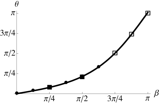
We have calculated the OMP angle $\theta$ using four different methods with excellent agreement (Fig. 1). First, we obtain $\theta$ from Eq. (4); this requires a smooth gauge for ${\cal A}$, which can be found using now-standard Wannier-based methods [22]. Results are shown for $\beta=\pi/4$ and $\beta=\pi/2$ (filled squares).

Next, we have calculated the polarization [16]

resulting from a single magnetic flux quantum in a large supercell. Varying the supercell size (and thereby $B$) allows us to approximate $dP/dB$, yielding the open squares in Fig. 1. The points in Fig. 1 are from the surface Hall response in a slab geometry, described below. Finally, to obtain the curve in Fig. 1, we also computed $\theta(\beta)$ from the second Chern expression [15, 12]

(derived above as Eq. (5)). Clearly, the various approaches are numerically equivalent.

We now discuss the surface Hall conductivity, whose fractional part in units of $e^{2}/h$ is just $\theta/2\pi$ [4]. Consider a material with coupling $\theta$ in a slab geometry that is finite in the ${\bf\hat{z}}$ direction and surrounded by $\theta=0$ vacuum. The simplest interfaces will then lead to $\sigma_{H}=\theta e^{2}/(2\pi h)$ at the top surface and $-\theta e^{2}/(2\pi h)$ at the bottom surface, for a total $\sigma_{xy}$ of zero. More generally, arbitrary surface quantum Hall layers change the total integer quantum Hall state, but not the fractional parts at each surface.

The spatial contributions to the Hall conductance in the slab geometry can be resolved as follows. The unit cell is a supercell containing some number $N$ of original unit cells in the ${\bf\hat{z}}$ direction, with translational invariance remaining in the ${\bf\hat{x}}$ and ${\bf\hat{y}}$ directions. The TKNN integer for the entire slab is [5, 23]

Here $i$ and $j$ take the values $k_{x}$ and $k_{y}$ and $\mathcal{P}=\sum_{\nu}|u_{\nu}\rangle\langle u_{\nu}|$ is the projection operator onto the occupied subspace ($\nu$ runs over occupied bands). To find how different ${\bf\hat{z}}$ layers contribute to $C$, define a projection $\tilde{\mathcal{P}}_{n}$ onto layer $n$ within the supercell, and compute

The results, presented in Fig. 2, confirm that the surface layers have half-integer Hall conductance when $\beta=\pi$ in (8) and that the sign on each surface is switched by local $T$-breaking perturbations (in this example, a uniform Zeeman coupling in the surface layer).

To gain some insight into the microscopic origin of $\theta$ in the noninteracting case, using Eq. (4) we have calculated $\theta$ for a Hamiltonian that breaks $PT$ (as well as $P$ and $T$) by adding a weak, uniform (i.e., not staggered) Zeeman coupling. For some values of $\beta$ this lifts all degeneracies, enabling us to isolate the single-band and interband contributions to $\theta$ and to verify that, because interband contributions are nonzero in general, $\theta$ is a property of the whole occupied spectrum (unlike polarization, which is a sum of individual band contributions). A single filled band can have nonzero $\theta$ only if there are more than two bands in total [24].

Experimental detection of $\theta$ is more difficult for a topological insulator than for a generic magnetoelectric insulator because some $T$-breaking perturbation is needed to gap the surface state. Furthermore, a large surface density of states, as in Bi_0.9Sb_0.1, may complicate the measurement: while even a weak magnetic field will in principle lead to a gap and half-integer quantum Hall effect at each surface, the large number of filled surface Landau levels may make it difficult to isolate the half-integer part of surface $\sigma_{\mathrm{H}}$. In the presence of broken discrete symmetries, as in antiferromagnets or multiferroics, the surface gap exists naturally and experiments are easier. For example, the theoretical methods of this paper could be used to compute the orbital part of the recently measured $\theta$ in Cr₂O₃ [3].

The authors acknowledge useful discussions with A. Selem and I. Souza. The work was supported by the Western Institute of Nanoelectronics (AME), NSF DMR-0804413 (JEM), and NSF DMR-0549198 (DV).

References

- [1] N. A. Spaldin and M. Fiebig, Science 309, 391 (2005).
- [2] M. Fiebig, J. Phys. D - Applied Phys. 38, R123 (2005).
- [3] F. W. Hehl, Y. N. Obukhov, J.-P. Rivera, and H. Schmid, Physics Letters A 372, 1141 (2008), eprint 0708.2069.
- [4] F. Wilczek, Phys. Rev. Lett. 58, 1799 (1987).
- [5] D. J. Thouless, M. Kohmoto, M. P. Nightingale, and M. den Nijs, Phys. Rev. Lett. 49, 405 (1982).
- [6] C. L. Kane and E. J. Mele, Phys. Rev. Lett. 95, 226801 (2005a).
- [7] C. L. Kane and E. J. Mele, Phys. Rev. Lett. 95, 146802 (2005b).
- [8] B. A. Bernevig, T. L. Hughes, and S.-C. Zhang, Science 314, 1757 (2006).
- [9] J. E. Moore and L. Balents, Phys. Rev. B 75, 121306(R) (2007).
- [10] R. Roy, cond-mat/0607531.
- [11] L. Fu, C. L. Kane, and E. J. Mele, Phys. Rev. Lett. 98, 106803 (2007).
- [12] X. Qi, T. L. Hughes, and S.-C. Zhang, Phys. Rev. B 78, 195424 (2008).
- [13] D. Hsieh, D. Qian, L. Wray, Y. Xia, Y. S. Hor, R. J. Cava, and M. Z. Hasan, Nature 452, 970 (2008).
- [14] L. Fu and C. L. Kane, Phys. Rev. B 76, 045302 (2007).
- [15] D. Xiao, J. Shi, D. P. Clougherty, and Q. Niu, Phys. Rev. Lett. 102, 087602 (2009).
- [16] R. D. King-Smith and D. Vanderbilt, Phys. Rev. B 47, 1651 (1993).
- [17] G. Ortiz and R. M. Martin, Phys. Rev. B 49, 14202 (1994).
- [18] T. Thonhauser, D. Ceresoli, D. Vanderbilt, and R. Resta, Phys. Rev. Lett. 95, 137205 (2005).
- [19] D. Xiao, J. Shi, and Q. Niu, Phys. Rev. Lett. 95, 137204 (2005).
- [20] M. Nakahara, Geometry, Topology and Physics (Institute of Physics Publishing (Bristol), 1998).
- [21] S.-S. Lee and S. Ryu, Physical Review Letters 100, 186807 (2008), eprint 0708.1639.
- [22] N. Marzari and D. Vanderbilt, Phys. Rev. B 56, 12847 (1997).
- [23] J. E. Avron, R. Seiler, and B. Simon, Phys. Rev. Lett. 51, 51 (1983).
- [24] J. E. Moore, Y. Ran, and X.-G. Wen, Physical Review Letters 101, 186805 (2008), eprint 0804.4527.