Liquid behavior of hot QGP in the finite temperature field theory
Abstract
In this paper, we compare the dispersion relations of hard thermal loop and complete one loop. It is shown that in the dynamical screening regime, the completely one-loop calculation presents a prominent threshold frequency, below which no pure imaginary mode survives. This phenomenon is responsible for the oscillatory static in-medium potential and ultimately results in a damping oscillation of the radial distribution function. We consider this typical shape is the footprint of liquid QGP.
pacs
12.38.Mh,11.10.WxI Introduction
The experiments of ultra-relativistic heavy ion collision at RHIC provide us a platform to study the quark-gluon plasma(QGP) signal as well as its novel properties. One of those surprises the scientists is the low viscous flow. At Au+Au 200GeV collision, the elliptic flow can be well fitted by an ideal hydrodynamics up to 2GeV of the transverse momenta[1, 2], which implies a perfect fluid behavior. This perfect behavior of QGP makes people consider it in a liquid state[3, 4], with the temperature slightly above the critical temperature . How to understand such a good liquid of QGP is a fundamental problem that attracts much attention. Some ideals and methods came from other fields, for example the AdS/CFT correspondence from the superstring theory and the physics of strongly coupled QED plasma. For more details, please refer to the report of E. Shuryak in Ref[5] and references therein.
In this paper, we try to investigate the radial distribution function of liquid QGP in the framework of finite temperature theory. Hard Thermal Loop(HTL) approximation and HTL resummation scheme were widely used in thermal field theory when discussing measurable medium effects such as Debye screening, collective modes, particle energy loss so on and so forth. The HTL physics were proved reliable in the temperature limit. For example, it can represent the correct collective modes in hot plasma[6]. The boson and fermion damping rates obtained in the HTL resummation scheme are positive and gauge invariant even in the non-abelian system[7, 8]. However, although the HTL has this and that good qualities, it has its own restrictions. The HTL approximation as well as the corresponding resummation scheme request the high temperature limit which is not a trivial condition for a real system like the QGP at . This temperature is obvious not reaching the high temperature limit so that the HTL scheme might be doubtful. To avoid such suspicion, one can adopt complete one loop scheme instead of HTL.
In this paper, we will start with QED plasma, comparing the dispersion relations of HTL and complete one loop, demonstrating their distinct screening behaviors. Then we will turn to the quark-gluon plasma, calculating the static in-medium inter-quark potential and the radial distribution function. The damping oscillatory radial distribution function suggests the QGP might be in a liquid state. Finally, we will discuss the general factors that decide the state of matter, pointing out a possible way to study the properties of QGP liquid.
II dispersion relation
Dispersion relation is a basic relation of many-particle system which carries essential physical information. A slight difference between dispersion relations may indicate totally different physics. In this section, we will compute the QED dispersion relations at HTL and completely one-loop level respectively. One will see the distinct dispersion curves in both dispersion regime and dynamic screening regime.
The dispersion relation is defined as the energy-moment relation at the pole of full boson propagator,
| (1) | |||
| (2) |
where and are the longitudinal and transverse components of boson polarization tensor respectively. In this paper we just take the longitudinal dispersion relation as an example and study the color-electric properties of hot plasma.
In HTL approximation,
| (3) |
where is the fine structure constant of QED. For a complete one loop,
| (4) | |||||
where , and is the electron mass. is the Fermi-Dirac distribution function with .
Inserting Eqs.(3) and (4) into Eq.(1) and figuring out the relation between and numerically, one could obtain FIG.1. This figure is plotted in not only the dispersion regime where the momentum is real, but also the dynamic screening regime where is pure imaginary. In FIG.1 the abscissa combines both regimes, separated by a zero line of . The right area to the zero line is for the common dispersion relation when the momenta are real. The left area, on the contrary, is the dynamic screening regime for pure imaginary momenta.
The HTL dispersion relation has been obtained and discussed in details[10]. We represent it in FIG.1 with dashed curves to compare with the complete one loop. However we do not intend to compare the whole regime, since the two curves in the normal dispersion regime behaves very similar. Instead, we would like to concern about the prominent difference in the dynamical regime. In this regime, the HTL curve reaches the abscissa, indicating a screening effect at zero frequency referred to the well-known Debye screening. While in the completely one-loop case, an threshold frequency shows up, below which no pure imaginary mode survives. That is to say a real part of the momentum is necessary and the dynamical screening described by the HTL [10] is broken up. Especially, in the static limit where , the plasma is not screened with Debye form contributed by the pure imaginary mode. Instead, the screening oscillates due to the complex mode in the completely one-loop calculation. We will see it in the next section.

III Oscillatory potential
So far the Debye screening picture has been changed in the completely one-loop calculation based on the dispersion analysis in last section, one would like to check the static potential and see how it will look like in the new picture.
In the relativistic plasma, the in-medium potential is explained by the skeleton diagram with full boson propagator, as shown in FIG.2. The shadowed circle denotes all possible polarizations. In math language, it is
| (5) |
where is the distance between two arbitrary electrons. To perform the integral in Eq.(5), one should construct a contour according to the analytic structure of the integrand, locating all poles within the contour on complex plane. We would like to point out here that the Eq.(5) is actually involving a resummation scheme, because the effective boson propagator is obtained from Dyson-Schwinger equation.

To demonstrate the general form of the potential contributed by poles, one can first define the pole as
| (6) |
where and are the real and imaginary parts of the pole. With this definition, one can perform the contour integral and find
| (7) |
where the sum includes all pole contributions. and are defined as the real and imaginary parts of the residue,
| (8) |
with the prime denoting .
Notice that the pole of the integral in Eq.(5) is nothing else but the point of on the dispersion curve. Due to the appearance of the threshold frequency in FIG.1, the potential from HTL polarization and completely one-loop polarization may behave differently. The HTL dispersion curve extends directly to zero frequency in the dynamic screening regime, which means the pole is purely imaginary with at the static limit. More explicitly,
| (9) |
and
| (10) |
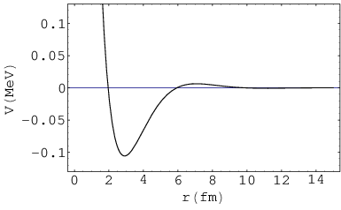
While on the completely one-loop dispersion curve, no pure imaginary solution is found at , which implies the pole contains both real and imaginary parts and the static potential takes the general form of damping oscillation shown as Eq.(7). One can find out the poles numerically by solving the equation
| (11) |
which is Eq.(1) in the static limit () where the mode .
In FIG.3 we demonstrated the oscillatory potential of QED. This damping oscillation is qualitatively different for the monotonic Debye potential in Eq.(10).
IV radial distribution function and liquid QGP
Generally speaking, In the picture of Debye screening, the in-medium particles are ”dressed” with the effective radii of Debye length. Therefore the interactions among the component particles are rather weak so that the system can be treated as the ideal gas. However, once the Debye potential is replaced by the oscillatory potential, the ideal gas is no longer a qualified model. Then what kind of state of matter is the oscillatory potential relevant to? To answer this question, one must know about the typical character of each state.
To identify different states of matter, one is to distinguish the different spacial configurations of the component particles. The so-called radial distribution function (RDF), which is the probability of finding two particles at a distance from each other, is introduced as a powerful tool. For instance, particles in the gas state are completely random, so that the possibilities of finding any two particles are almost the same. Therefore its RDF remains constant11 1 The monotonic increasing is due to the inaccessible core of the component particle. as shown in FIG.4. While the particles in the liquid state have short range order so that the possibilities of finding nearby particles are much larger than those far particles. Accordingly, the RDF in the liquid state will present several damping peaks along the radial direction[11, 12, 13] which is also sketched in FIG.4. We consider this damping oscillation shape as the basic characteristic of a liquid state, in other words, if someone could obtain such kind of RDF, he may discover the footprint of a liquid state. Thoma[14] calculated the RDF of QGP in the HTL scheme, which gives the exact Debye screening, and confirmed the negative result for identifying a liquid. In the following, we will give up the HTL scheme and work with complete one loop.

In the liquid state theory, one can define the RDF through
| (12) |
where is nothing else but the in-medium potential of average inter-particle forces[12]. In the classical liquid state theory, the RDF can be obtained analytically through a certain pair potential model including the often used Hypernetted-chain(HNC) or Percus-Yevick(PY) approximations, or through some computer simulations like Monte Carlo or Molecular dynamics[11]. In this paper, we follow none of those schemes, instead, we adopt the static in-medium potential obtained in the completely one-loop calculation referring to the last section.

As for plain QCD, the one-loop gluon polarization is determined by the diagrams in FIG.5. Compared with QED, QCD involves the gluon self-coupling. One can calculate the temperature-dependent polarization tensor in the framework of thermal field theory, like what we do in the last section. We skip the standard steps and directly present the expressions of completely one-loop polarization tensor of QCD in the temporary axis gauge (TAG) as[15]
| (13) | |||
| (14) |
where is the quark mass. is the gluon distribution function. Here we study the 2-flavor QGP. For the running coupling , we use the two-loop renormalization group expression[21]
| (15) |
where MeV for the temperature range .
We would like to point out that although applying the linear response theory to non-Abelian gauge theory is at the risk of gauge noninvariance, the TAG is believed safe enough because in this gauge one can obtain the same vacuum polarization corrected effective charge as the renormalization group charge[15]. We hope the discussion in TAG may give at least the qualitative features of the potential and RDF.
Adding up Eqs.(13) and (14) and inserting them into Eq.(5), one can find out the pole numerically. Then the interquark potential (7) is obtained and so as to the RDF considering Eq.(12). FIG.6 is the RDF of QCD plasma where we choose two different temperatures 0.2 and 0.3GeV.22 2 The deconfined QGP is a Coulomb-like plasma, whose dimensionless coupling parameter is where is the eignvalue of the Casimir operator for quark and antiquark, is the particle number density. For estimation, we take for 2-flavor QGP by considering it as a massless gas[22, 23] For T=0.2 and 0.3GeV, the running coupling constants are 0.5 and 0.35, and the corresponding coupling parameters are 2.0 and 1.4, which are great than 1, indicating a liquid state. In FIG.6, one can see clearly the damping oscillatory behavior of the RDF, which is very similar to the typical shape of liquid in FIG.4. This result might indicate the liquid state of hot QGP. Furthermore, the RDF oscillation becomes weaker and weaker with the increase of temperature, thus one may expect the QGP is approaching to an ideal gas at the high temperature limit.

V discussion
In this paper, we start with the comparison of dispersion relations of HTL and complete one loop, pointing out an important discrepancy in the dynamical screening regime which results in the different behaviors of the static in-medium potentials. Then we discuss the RDF of hot QGP. It appears an obvious damping oscillation which implies the QGP might be in a liquid state.
How to deal with the interacting many-body system, especially the strongly coupled or strongly correlated system, is a rather difficult but fundamental problem. In principle, one can reduce the many-particle distribution function to two- or single-particle distribution function[24]. The RDF is actually the two-particle distribution function. It is the basic physical quantity in the atomic liquid theory that has been related to various kinetic and thermodynamic observables[11, 12]. On one hand, the RDF is obtained by considering certain dynamical and thermal statistical model from the theoretical aspects. On the other hand, it can be measured through scattering experiments in the atomic liquid. Compare the theoretical RDF and the RDF extracted from experiments, then one can figure out deeper discipline that rules over the phenomenon. Parallel to the classical liquid theory, the RDF in this paper is the static two-quark distribution function with spherical symmetry. Although we can not measure the quark distribution in QGP through scattering experiment as we do to the atomic liquid, we can still measure the density-density correlations, which is relevant to the Fourier transformation of RDF[14], by observing the final state distributions. We hope in this way, the picture in our calculation can be tested by the experiments.
Acknowledgements.
This work is partly supported by the National Natural Science Foundation of China under project Nos. 10747135, 10675052 and 10575043.References
- [1] STAR collaboration, Phys. Rev. Lett. 90 (2003) 032301
- [2] PHENIX collaboration, Phys. Rev. Lett. 91 (2003)182301
- [3] M.H. Thoma, J. Phys. G 31, L7 (2005); Erratum, J. Phys. G 31, 539 (2005)
- [4] A. Peshier and W. Cassing, Phys. Rev. Lett. 94, 172301 (2005)
- [5] E. Shuryak, arXiv:0807.3033v1
- [6] M. Le Bellac, Thermal Field Theory (Cambridge Univ. Press, Cambridge, 1996)
- [7] R.D. Pisarski, Phys. Rev. Lett. 63, 1129 (1989)
- [8] E. Braaten and R.D. Pisarski, Phys. Rev. D, 42, 2156 (1990)
- [9] E.V. Shuryak and I. Zahed, Phys. Rev. C 70, 021901(R) (2004)
- [10] H.A. Weldon, Phys. Rev. D, 26, 1394 (1982)
- [11] N.H. March and M.P. Tosi, Introduction to Liquid State Physics (World Scientific Publishing, Singapore 2002)
- [12] P.A. Egelstaff, An Introduction to the Liquid State (Clarendon Press, Oxford 1992)
- [13] S. Ichimaru, Rev. Mod. Phys. 54, 1017 (1982)
- [14] M.H. Thoma, Phys. Rev. D 72, 094030 (2005)
- [15] J.I. Kapusta, Finite Temperature Field Theory (Cambridge Univ. Press, Cambridge, 1989)
- [16] J. Diaz Alonso, A. Pérez and H. Sivak, Nucl. Phys. A 505, 695 (1989)
- [17] J. Diaz Alonso, E. Gallego and A. Pérez, Phys. Rev. Lett. 73, 2536 (1994)
- [18] J. Kapusta and T. Toimela, Phys. Rev. D 37, 3731 (1988)
- [19] A. L. Fetter and J. D.Wakecka, Quantum Theory of Many Particle Systems (McGraw-Hill, New York, 1971)
- [20] H. Sivak, A. Pérez and J. Diaz Alonso, Prog. Theor. Phys. 105, 961 (2001)
- [21] O. Kaczmarek and F. Zantow, Phys. Rev. D 71, 114510 (2005)
- [22] B.A. Gelman, E.V. Shuryak and I. Zahed, Phys. Rev. C 74, 044908 (2006)
- [23] M.H. Thoma, J. Phys. G 31, L7 (2005); ibid 31, 539 (2005)
- [24] F. Mohling, Statistical Mechanics: Methods and Applications (Publishers Creative Services Inc., 1982)