跳到论文正文
W Papers独立论文阅读器 arXiv:0810.2815 论文正文 计算阅读时间 · 0%
引用这篇论文根据当前论文元数据生成,正式投稿前建议核对。


License: arXiv.org perpetual non-exclusive license
arXiv:0810.2815v2 [physics.flu-dyn] 24 Feb 2011

Nonmodal amplification of stochastic disturbances
in strongly elastic channel flows

Journal: J. Non-Newtonian Fluid Mech.
Mihailo R. Jovanović Email: mihailo@umn.edu URL: http://www.umn.edu/$∼$mihailo Address: Department of Electrical and Computer Engineering, University of Minnesota, Minneapolis, MN 55455, USA    Satish Kumar Email: kumar030@umn.edu URL: http://www.cems.umn.edu/research/kumar/kumar.htm Address: Department of Chemical Engineering and Materials Science, University of Minnesota, Minneapolis, MN 55455, USA
Abstract

Nonmodal amplification of stochastic disturbances in elasticity-dominated channel flows of Oldroyd-B fluids is analyzed in this work. For streamwise-constant flows with high elasticity numbers μ\mu and finite Weissenberg numbers W​eW\!e, we show that the linearized dynamics can be decomposed into slow and fast subsystems, and establish analytically that the steady-state variances of velocity and polymer stress fluctuations scale as 𝒪⁡(W​e2){\cal O}(W\!e^{2}) and 𝒪⁡(W​e4){\cal O}(W\!e^{4}), respectively. This demonstrates that large velocity variance can be sustained even in weakly inertial stochastically driven channel flows of viscoelastic fluids. We further show that the wall-normal and spanwise forces have the strongest impact on the flow fluctuations, and that the influence of these forces is largest on the fluctuations in streamwise velocity and the streamwise component of the polymer stress tensor. The underlying physical mechanism involves polymer stretching that introduces a lift-up of flow fluctuations similar to vortex tilting in inertia-dominated flows. The validity of our analytical results is confirmed in stochastic simulations. The phenomenon examined here provides a possible route for the early stages of a bypass transition to elastic turbulence and might be exploited to enhance mixing in microfluidic devices.

Keywords: 
Elastic turbulence , frequency responses , inertialess flows , polymer stretching , singular perturbations , variance amplification , viscoelastic fluids.

1 Introduction

1.1 Background

The classical approach to transition to turbulence examines the linearized equations for exponentially growing normal modes. The existence of these unstable modes implies exponential growth of infinitesimal perturbations to the laminar flow, and the corresponding eigenfunctions identify flow patterns that are expected to dominate early stages of transition. This approach agrees with experiments in many flows (e.g., those driven by thermal and centrifugal forces [1]) but it comes up short in matching experimental observations in wall-bounded shear flows (flows in channels, pipes, and boundary layers). The failure of hydrodynamic stability analysis in describing the early stages of transition is attributed in part to the nonnormal nature of the linearized equations, which may manifest itself by transient growth of perturbations [2, 3], protrusion of pseudospectra to the unstable regions [1, 4], and large receptivity to ambient disturbances [5, 6, 7]. Even in stable regimes – owing to nonnormality – perturbations that grow transiently before decaying due to viscosity can be configured, irregularities in laboratory design can lead to instability, and disturbances (such as free-stream turbulence or surface imperfections) can be amplified by orders of magnitude. These conclusions can be reached by performing transient growth, pseudospectra, or variance amplification analyses [8, 9, 10]. All of these methods demonstrate the importance of streamwise-elongated flow patterns of high and low streamwise velocity (streaks) in transitional wall-bounded shear flows of Newtonian fluids; this is at odds with modal stability results, but in agreement with experiments [11] and direct numerical simulations [12] conducted in noisy environments. We note that in order to understand the later stages of transition, consideration of nonlinear interactions between streamwise-varying fluctuations and the streaks is required [13, 14, 15].

Transition to turbulence in viscoelastic fluids is important from both fundamental and technological perspectives [16]. The observation that transition can occur even when the effects of fluid elasticity dominate those of inertia – which is a primary cause of transition in Newtonian fluids – is particularly intriguing [17, 18, 19, 20, 21, 22]. Improved understanding of transition mechanisms in viscoelastic fluids has broad applications, ranging from deeper insight into order-disorder transitions in spatially extended nonlinear dynamical systems to enhanced mixing in microfluidic devices through the addition of polymers [23, 19]. The phenomenon of ‘elastic turbulence’ occurs in the absence of inertial effects [17], and it has been observed experimentally in shear flows with curved streamlines [17, 18, 19, 24, 25, 26]. The transition in curvilinear flows is triggered by a purely elastic instability that originates from the interactions between polymer stress fluctuations and the velocity gradients in the base flow [27, 16, 28]. Currently, it is not known whether fluid elasticity can promote transition in parallel shear flows with negligible inertial forces.

In spite of the linear stability of weakly inertial parallel shear flows of viscoelastic fluids, small fluctuations around the laminar base state can achieve significant transient growth. Early efforts used simulations of two-dimensional (2D) channel flows to probe their transient responses in both linear and nonlinear regimes [29, 30]. A new family of linearly stable transiently growing 2D stress modes was identified for the Oldroyd-B constitutive model [31]; these modes were obtained in Couette flow by setting the velocity and pressure fluctuations to zero and they do not couple back to the momentum equation. More recently, a similar result was shown for the three-dimensional (3D) upper convected Maxwell model (a special case of the Oldroyd-B model) with linear base velocity [32]. In [33], an exact solution to the Oldroyd-B model was constructed which displays non-monotonic transient responses in strongly elastic 2D Couette flow with arbitrarily low, but non-zero, inertia. Even in channel flows without inertia, the streamwise-independent velocity and stress fluctuations can exhibit transient growth that scales unfavorably with elasticity [34]. Several explicit scaling relationships were established, and computations were used to identify the spatial structure of the initial conditions (in the polymer stress components) that grow the most with time.

Amplification of stochastic disturbances in channel flows of viscoelastic fluids was recently examined using linear systems theory [35]. For the Oldroyd-B model, computations reported in [35] demonstrated that streamwise-constant velocity fluctuations can experience considerable amplification even in the weakly inertial/strongly elastic regime. As in Newtonian fluids, this amplification is fundamentally nonmodal in nature: it cannot be described using the normal mode decomposition of classical hydrodynamic stability analysis [8, 9, 10]. Rather, it arises from an energy exchange involving the fluctuations in the streamwise/wall-normal polymer stress and the wall-normal gradient of the streamwise velocity [36].

Despite this recent progress, analytical results that describe amplification of stochastic disturbances in strongly elastic channel flows of viscoelastic fluids are lacking. Such results are important because of the physical insight they yield, and as a means to validate numerical simulations. The purpose of the present work is to address this issue.

1.2 Preview of key results

The key parameters that characterize channel flows of viscoelastic fluids are: the viscosity ratio, β=ηs/(ηs+ηp)\beta=\eta_{s}/(\eta_{s}+\eta_{p}), where ηs\eta_{s} and ηp\eta_{p} are the solvent and polymer viscosities; the Weissenberg number, W​e=λ​Uo/LW\!e=\lambda U_{o}/L, which represents the product of the polymer relaxation time λ\lambda and the typical velocity gradient Uo/LU_{o}/L; and the elasticity number, μ=W​e/R​e\mu=W\!e/Re, which quantifies the ratio of the polymer relaxation time λ\lambda to the viscous diffusion time ρ​L2/(ηs+ηp)\rho L^{2}/(\eta_{s}+\eta_{p}). Here, R​e=ρ​Uo​L/(ηs+ηp)Re=\rho U_{o}L/(\eta_{s}+\eta_{p}) is the Reynolds number, which represents the ratio of inertial to viscous forces, UoU_{o} is the largest base velocity, LL is the channel half-height, and ρ\rho is the fluid density. By modeling ambient disturbances to streamwise-constant channel flows of Oldroyd-B fluids (with spanwise wavenumber kzk_{z}) as an additive white Gaussian forcing with zero mean and unit variance, we develop an explicit scaling of the variance (or energy) amplification of velocity fluctuations with the Weissenberg number W​eW\!e,

Ev​(kz,W​e,β,μ)=f⁡(kz,β,μ)+W​e2​g​(kz,β,μ).E_{\mathrm{v}}(k_{z};W\!e,\beta,\mu)\;=\;f(k_{z};\beta,\mu)\;+\;W\!e^{2}\,g(k_{z};\beta,\mu). (1)

Here, ff and gg denote W​eW\!e-independent functions where gg accounts for the amplification from wall-normal and spanwise forces to the fluctuations in streamwise velocity, while ff accounts for the amplification from all other forcing to all other velocity components. It is worth noting that EvE_{\mathrm{v}} quantifies the ensemble-average energy density (associated with the velocity field) of the statistical steady-state [5], and it is determined by integrating the power spectral density over all temporal frequencies [37].

Furthermore, considering flows with μ≫1\mu\gg 1, we apply singular perturbation techniques to establish that the steady-state velocity variance scales as

Ev​(kz,W​e,β,μ)=μ​f~0​(kz)/β+f~1​(kz)​(1−β)/β2+W​e2​g~0​(kz)​(1−β)2/β+𝒪⁡(1/μ).E_{\mathrm{v}}(k_{z};W\!e,\beta,\mu)\;=\;\mu\tilde{f}_{0}(k_{z})/\beta\;+\;\tilde{f}_{1}(k_{z})\,(1-\beta)/\beta^{2}\;+\;W\!e^{2}\,\tilde{g}_{0}(k_{z})\,(1-\beta)^{2}/\beta\;+\;{\cal O}(1/\mu).

Our analysis demonstrates that, in flows with high elasticity numbers, the linear μ\mu-scaling of the function ff in (1) arises from the corresponding power spectral density becoming almost uniformly distributed over the temporal frequency band whose width is proportional to μ\mu. We also show that, from a physical point of view, no important viscoelastic effects take place in the contribution of the function f~0\tilde{f}_{0} to the variance amplification.

The last expression should be compared to the expression for the variance amplification in Newtonian fluids [6],

EN​(kz,R​e)=fN​(kz)+R​e2​gN​(kz).E_{N}(k_{z};Re)\;=\;f_{N}(k_{z})\;+\;Re^{2}\,g_{N}(k_{z}). (2)

At low R​eRe the kzk_{z}-dependence of ENE_{N} is governed by fN​(kz)f_{N}(k_{z}), EN​(kz,R​e)≈fN​(kz),E_{N}(k_{z};Re)\approx f_{N}(k_{z}), and at high R​eRe it is governed by gN​(kz)g_{N}(k_{z}), EN​(kz)≈R​e2​gN​(kz)E_{N}(k_{z})\approx Re^{2}\,g_{N}(k_{z}). In this paper, we show that f~0​(kz)=fN​(kz)\tilde{f}_{0}(k_{z})=f_{N}(k_{z}) which implies that the kzk_{z}-dependence of f~0\tilde{f}_{0} is characterized by viscous dissipation [6]. This clearly indicates that, at the level of velocity fluctuation dynamics, the behavior of Newtonian fluids with low R​eRe and the behavior of Oldroyd-B fluids with low W​eW\!e is dominated by diffusion. On the other hand, the gg-functions in the expressions for EvE_{\mathrm{v}} and ENE_{N} exhibit peaks at kz=𝒪⁡(1)k_{z}={\cal O}(1); the values of kzk_{z} where these peaks take place identify the spanwise length scales of the most energetic response of velocity fluctuations to stochastic forcing in Newtonian fluids with high R​eRe, and in Oldroyd-B fluids with high W​eW\!e.

We note that gN​(kz)g_{N}(k_{z}) and g~0​(kz)\tilde{g}_{0}(k_{z}) arise from fundamentally different physical mechanisms: in inertia-dominated flows of Newtonian fluids, vortex tilting is the main driving force for amplification; in elasticity-dominated flows of viscoelastic fluids, it is polymer stretching, which gives rise to an energy transfer from the base flow to fluctuations. In streamwise-constant channel flows of Newtonian fluids, the linearized dynamics of the wall-normal vorticity, η\eta, are governed by [2]

∂tη=−ReU′(y)∂zv+Δη,\partial_{t}\eta\;=\,-Re\,U^{\prime}(y)\,\partial_{z}v\;+\;\Delta\eta, (3)

where vv denotes the wall-normal velocity fluctuations, Δ\Delta is a Laplacian, and −U′​(y)-U^{\prime}(y) is the base flow vorticity (in the spanwise direction zz). The first term on the right-hand side of (3) represents the linearized vortex-tilting term which acts as a source in the vorticity equation. From a physical point of view, the spanwise vorticity of the base flow, i.e. −U′​(y)-U^{\prime}(y), gets tilted in the wall-normal direction yy by the spanwise changes in vv which leads to the amplification of the wall-normal vorticity (and thereby streamwise velocity, η=∂zu\eta=\partial_{z}u) [2]. In this paper, we show that the linearized wall-normal vorticity equation in inertialess streamwise-constant flows of Oldroyd-B fluids assumes the following form

∂tΔ​η\displaystyle\partial_{t}\Delta\eta =−We(1/β−1)(U′(y)Δ∂z+ 2U′′(y)∂y​z)ϑ−(1/β)Δη\displaystyle\;=\,-W\!e\left(1/\beta-1\right)\left(U^{\prime}(y)\,\Delta\,\partial_{z}\,+\,2\,U^{\prime\prime}(y)\,\partial_{yz}\right)\vartheta\;-\;\left(1/\beta\right)\Delta\eta (4a)
=−W​e​(1/β−1)​(∂y​z(U′​(y)​τ22)+∂z​z(U′​(y)​τ23))−(1/β)​Δ​η,\displaystyle\;=\,-W\!e\left(1/\beta-1\right)\left(\partial_{yz}\left(U^{\prime}(y)\tau_{22}\right)\,+\,\partial_{zz}\left(U^{\prime}(y)\tau_{23}\right)\right)\;-\;\left(1/\beta\right)\Delta\eta, (4b)

where ϑ\vartheta in (4a) is obtained by filtering high temporal frequencies in the wall-normal velocity vv; see Section 4.1 for details. The terms U′​(y)​τ22U^{\prime}(y)\tau_{22} and U′​(y)​τ23U^{\prime}(y)\tau_{23} in (4b) represent stretching of the corresponding stress fluctuations by a background shear; gradients of these quantities provide a source in the vorticity equation even in the absence of inertia. Thus, base-shear stretching of stress fluctuations along with their spanwise variations gives rise to the amplification of η\eta (and consequently uu) in inertialess flows of viscoelastic fluids. As in streamwise-constant inertial flows of Newtonian fluids, this amplification disappears either in the absence of spanwise variations in flow fluctuations, i.e. ∂z(⋅)=0\partial_{z}(\cdot)=0, or in the absence of the background shear, i.e. U′=0U^{\prime}=0.

Additional insight into the above mechanism can be gained by considering the momentum conservation equation in planes perpendicular to the direction of the base flow. For streamwise-independent inertialess flows, there is a static-in-time relationship between the (y,zy,z)-gradients in τ22\tau_{22}, τ23\tau_{23}, and τ33\tau_{33} and the wall-normal (vv) and spanwise (ww) velocity fluctuations

0=−∂yp+(1−β)(∂yτ22+∂zτ23)+βΔv+d2,0=−∂zp+(1−β)(∂yτ23+∂zτ33)+βΔw+d3.\begin{array}[]{rcl}0&\!\!=&-\partial_{y}\,p\,+\,(1-\beta)\left(\partial_{y}\tau_{22}\,+\,\partial_{z}\tau_{23}\right)\,+\,\beta\,\Delta v\,+\,d_{2},\\[2.84544pt] 0&\!\!=&-\partial_{z}\,p\,+\,(1-\beta)\left(\partial_{y}\tau_{23}\,+\,\partial_{z}\tau_{33}\right)\,+\,\beta\,\Delta w\,+\,d_{3}.\end{array}

Spatial variations in vv and ww induced by these stress gradients result in streamwise vorticity fluctuations (i.e., the streamwise ‘rolls’); these redistribute momentum in the (y,zy,z)-plane and promote amplification of streamwise velocity fluctuations. As in the Newtonian case, this momentum exchange involves lifting of the low speed fluid away from the wall and movement of the high speed fluid towards the wall, and it is responsible for creation of low and high speed streaks that alternate in the spanwise direction. From a microscopic point of view, the end-to-end vectors of the elastic dumbbells that underlie the Oldroyd-B model are oriented in the streamwise direction in the base flow (the only non-zero diagonal element of the base polymer stress tensor is the streamwise component) [38, 39]. Stochastic forcing (d2,d3)(d_{2},d_{3}) perturbs the end-to-end vector and generates fluctuations in τ22\tau_{22}, τ23\tau_{23}, and τ33\tau_{33} (which are zero in the base flow). These fluctuations then lead to energy amplification through the mechanism described above; see Figure 1 for additional illustration.

Our second key result is an explicit formula for the steady-state variance maintained in the components of the polymer stress tensor by streamwise-constant stochastic forcing

Eτ​(kz,W​e,β,μ)=a⁡(kz,β,μ)+W​e2​b​(kz,β,μ)+W​e4​c​(kz,β,μ).E_{\tau}(k_{z};W\!e,\beta,\mu)\;=\;a(k_{z};\beta,\mu)\;+\;W\!e^{2}\,b(k_{z};\beta,\mu)\;+\;W\!e^{4}\,c(k_{z};\beta,\mu).

Here, aa, bb, and cc represent W​eW\!e-independent functions which in flows with high μ\mu also become elasticity-number-independent,

Eτ​(kz,W​e,β,μ)=a0​(kz,β)+W​e2​b0​(kz,β)+W​e4​c0​(kz,β)+𝒪⁡(1/μ).E_{\tau}(k_{z};W\!e,\beta,\mu)\;=\;a_{0}(k_{z};\beta)\;+\;W\!e^{2}\,b_{0}(k_{z};\beta)\;+\;W\!e^{4}\,c_{0}(k_{z};\beta)\;+\;{\cal O}(1/\mu).

We note that the cc-function, which primarily originates from the polymer stretching, quantifies the amplification from the wall-normal and spanwise forces to the fluctuations in the streamwise component of the polymer stress tensor, τ11\tau_{11}. Therefore, in high-W​eW\!e regimes the wall-normal and spanwise disturbances have the strongest influence, and the impact of these forces is largest on the streamwise velocity and polymer stress fluctuations. Furthermore, we demonstrate that, in flows with high elasticity numbers, the analysis of inertialess (or creeping) flows of Oldroyd-B fluids correctly predicts all important properties of the functions aa, bb, cc, and gg. On the other hand, the inertialess model provides a poor approximation at high temporal frequencies of the power spectral densities responsible for the generation of the function ff in (1). In fact, we show that the problem of determining this function in inertialess flows becomes ill-posed. This ill-posedness arises from the absence of the inertial terms in the momentum equation and it cannot be alleviated by the addition of diffusion to the constitutive equations.

Refer to caption
(a)
Refer to caption
(b)
Refer to caption
(c)
Figure 1: (a) The steady-state configuration of an elastic dumbbell is perturbed out of the (x,yx,y)-plane by stochastic forcing. (b) A projection of a perturbed dumbbell in the (y,zy,z)-plane. Dumbbell stretching in the wall-normal and spanwise directions creates fluctuations in polymer stress components τ22\tau_{22}, τ23\tau_{23}, and τ33\tau_{33}. (c) Streamwise vortices, generated by the gradients in τ22\tau_{22}, τ23\tau_{23}, and τ33\tau_{33}, induce streamwise streaks through the lift-up mechanism. A spanwise momentum exchange is enabled by displacement of fluid particles in the wall-normal direction.

The above analytical results are obtained as a consequence of our discovery that the linearized dynamics can be decomposed into slow and fast subsystems. This observation is used to cast the equations into a standard singularly perturbed form for which existing methodology [40] can be applied. The decomposition of the linearized dynamics at high μ\mu is not obvious a priori, and it takes advantage of the intrinsic time scale (λ\lambda) in the Oldroyd-B constitutive equation. In addition, it facilitates derivation of the explicit analytical expressions for the steady-state variances of velocity and polymer stress fluctuations given above. Our success with uncovering the hitherto unknown dependence of the energy amplification on the Weissenberg and elasticity numbers points to the scaling and modeling steps as prerequisites for applying standard singular perturbation techniques.

The organization of the rest of the paper is laid out next. In Section 2, we describe the streamwise-constant linearized model with forcing. In Section 3, we provide explicit scaling of the frequency responses from different forcing to different velocity and stress components with the Weissenberg number. In Section 4, we provide analytical expressions for the variance amplification and discuss physical mechanisms leading to amplification from forcing to flow fluctuation components. We also determine the spanwise length scales of flow structures that contribute most to the steady-state variance and show that the most energetic velocity fluctuations assume the form of high and low speed streaks. In Section 5, we use stochastic simulations of the linearized dynamics to verify our analytical developments. The major contributions are summarized in Section 6 and the mathematical developments are relegated to the appendices. These developments make heavy use of singular perturbation techniques for stochastically forced linear systems and they provide important physical insight about the dynamics of strongly elastic fluids through transformation of the linearized equations into slow and fast subsystems.

2 The streamwise-constant linearized model with forcing

We consider incompressible channel flows of Oldroyd-B fluids with ϵ=1/μ≪1\epsilon=1/\mu\ll 1; see Figure 2 for geometry. The equations governing the dynamics (up to first order) of velocity (𝐯=[u​v​w]T{\bf v}=\left[\,u\,\,\,v\,\,\,w\,\right]^{T}), pressure (pp), and polymer stress tensor (𝝉\tau) fluctuations around base flow (𝐯¯,𝝉¯\overline{{\bf v}},\overline{\mbox{\boldmath$\tau$}}) are brought to a non-dimensional form by scaling time with λ\lambda, length with LL, velocity with UoU_{o}, polymer stresses with ηp​Uo/L\eta_{p}U_{o}/L, pressure with (ηs+ηp)​Uo/L(\eta_{s}+\eta_{p})U_{o}/L, and forcing per unit mass with (ηs+ηp)​Uo/ρ​L2(\eta_{s}+\eta_{p})U_{o}/\rho L^{2}

ϵ​𝐯˙=−ϵWe(∇𝐯𝐯¯+∇𝐯¯𝐯)−∇p+(1−β)∇⋅𝝉+β∇2𝐯+𝐝,0=∇⋅𝐯,𝝉˙=∇𝐯+(∇𝐯)T−𝝉+W​e​(𝝉⋅∇𝐯¯+𝝉¯⋅∇𝐯+(𝝉¯⋅∇𝐯)T+(𝝉⋅∇𝐯¯)T−∇𝐯𝝉¯−∇𝐯¯𝝉).\begin{array}[]{rcl}\!\!\!\epsilon\dot{{\bf v}}&\!\!\!\!=&-\epsilon\,W\!e\left(\mbox{\boldmath$\nabla$}_{\bf v}\overline{{\bf v}}+\mbox{\boldmath$\nabla$}_{\overline{{\bf v}}}\,{\bf v}\right)\,-\,\mbox{\boldmath$\nabla$}p\,+\,(1-\beta)\mbox{\boldmath$\nabla$}\!\cdot\!\mbox{\boldmath$\tau$}+\beta\mbox{\boldmath$\nabla$}^{2}{\bf v}\,+\,{\bf d},\\[2.84544pt] \!\!\!0&\!\!\!\!=&\mbox{\boldmath$\nabla$}\!\cdot\!{\bf v},\\[2.84544pt] \!\!\!\dot{\mbox{\boldmath$\tau$}}&\!\!\!=&\mbox{\boldmath$\nabla$}{\bf v}+\left(\mbox{\boldmath$\nabla$}{\bf v}\right)^{T}-\mbox{\boldmath$\tau$}+W\!e\bigl(\mbox{\boldmath$\tau$}\!\cdot\!\mbox{\boldmath$\nabla$}\overline{{\bf v}}+\overline{\mbox{\boldmath$\tau$}}\!\cdot\!\mbox{\boldmath$\nabla$}{\bf v}+(\overline{\mbox{\boldmath$\tau$}}\!\cdot\!\mbox{\boldmath$\nabla$}{\bf v})^{T}+(\mbox{\boldmath$\tau$}\!\cdot\!\mbox{\boldmath$\nabla$}\overline{{\bf v}})^{T}-\mbox{\boldmath$\nabla$}_{\bf v}\overline{\mbox{\boldmath$\tau$}}-\mbox{\boldmath$\nabla$}_{\overline{{\bf v}}}\,\mbox{\boldmath$\tau$}\bigr).\end{array} (5)

Here, a dot signifies a partial derivative with respect to time tt, ∇\nabla is the gradient, ∇𝐯=𝐯⋅∇\mbox{\boldmath$\nabla$}_{\bf v}={\bf v}\cdot\mbox{\boldmath$\nabla$}, and uu, vv, and ww are the velocity fluctuations in the streamwise (xx), wall-normal (yy), and spanwise (zz) directions, respectively. The linearized momentum equation is driven by the body force fluctuation vector 𝐝{\bf d}, which is purely harmonic in the horizontal directions, and stochastic in the wall-normal direction and in time,

𝐝⁡(x,y,z,t)=ℜ⁡(𝐝⁡(kx,y,kz,t)​ei⁡(kx​x+kz​z)),{\bf d}(x,y,z,t)\;=\;\Re\left({\bf d}(k_{x},y,k_{z},t)\,\mathrm{e}^{\mathrm{i}(k_{x}x\,+\,k_{z}z)}\right),

where the same notation is used to represent the field 𝐝⁡(x,y,z,t){\bf d}(x,y,z,t) and its Fourier transform in the horizontal directions 𝐝⁡(kx,y,kz,t){\bf d}(k_{x},y,k_{z},t); the difference between the two should be clear from the context. This spatio-temporal forcing will in turn yield velocity and polymer stress fluctuations of the same nature. We assume that 𝐝⁡(kx,y,kz,t){\bf d}(k_{x},y,k_{z},t) is a temporally stationary white Gaussian process with zero mean and unit variance; see [5, 6, 7] for additional details.
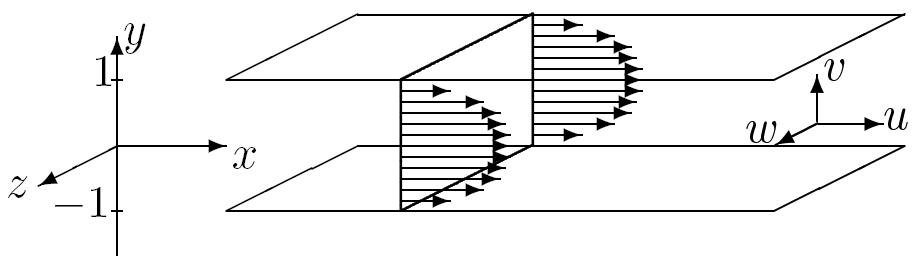
Refer to caption
Figure 2: Schematic of channel flow. In this paper, we study the linearized model for streamwise-constant three-dimensional fluctuations, which means that the dynamics evolve in the (y,zy,z)-plane, but fluctuations in all three spatial directions are considered.

We study the linearized model for streamwise-constant three-dimensional fluctuations, which means that the dynamics evolve in the (y,zy,z)-plane, but fluctuations in all three spatial directions are considered. This model is analyzed since the largest velocity variance in stochastically forced channel flows of viscoelastic fluids is maintained by streamwise-constant fluctuations [35]. The linearized equations can be brought to an evolution form by removing pressure from the equations and by expressing 𝐯{\bf v} in terms of the streamwise velocity and the (y,zy,z)-plane streamfunction fluctuations, {u=u\{u=u, v=∂zψv=\partial_{z}\psi, w=−∂yψ}w=-\partial_{y}\psi\}. By denoting

ϕ1=ψ,ϕ3=u,\phi_{1}\,=\,\psi,~~~\phi_{3}\,=\,u,

and by rearranging the polymer stress tensor components into

ϕ2=[τ22​τ23​τ33]T,ϕ4=[τ12​τ13]T,ϕ5=τ11,\mbox{\boldmath$\phi$}_{2}\,=\,\left[\,\tau_{22}\,\,\,\tau_{23}\,\,\,\tau_{33}\,\right]^{T},~~~\mbox{\boldmath$\phi$}_{4}\,=\,\left[\,\tau_{12}\,\,\,\tau_{13}\,\right]^{T},~~~\phi_{5}\,=\,\tau_{11},

system (5) with fluctuations that are constant in the streamwise direction (∂x(⋅)≡0\partial_{x}(\cdot)\equiv 0) and purely harmonic in the spanwise direction can be converted to

ϵ​ϕ˙1\displaystyle\epsilon\,\dot{\phi}_{1} =β​𝐒11​ϕ1+(1−β)​𝐒12​ϕ2+𝐅2​d2+𝐅3​d3,\displaystyle\;=\;\beta\,\mathbf{S}_{11}\,\phi_{1}\;+\;(1\,-\,\beta)\,\mathbf{S}_{12}\,\mbox{\boldmath$\phi$}_{2}\;+\;\mathbf{F}_{2}\,d_{2}\,+\,\mathbf{F}_{3}\,d_{3}, (6a)
ϕ˙2\displaystyle\dot{\mbox{\boldmath$\phi$}}_{2} =−ϕ2+𝐒21​ϕ1,\displaystyle\;=\;-\,\mbox{\boldmath$\phi$}_{2}\;+\;\mathbf{S}_{21}\,\phi_{1}, (6b)
ϵ​ϕ˙3\displaystyle\epsilon\,\dot{\phi}_{3} =β​𝐒33​ϕ3+ϵ​W​e​𝐒31​ϕ1+(1−β)​𝐒34​ϕ4+𝐅1​d1,\displaystyle\;=\;\beta\,\mathbf{S}_{33}\,\phi_{3}\;+\;\epsilon\,W\!e\,\mathbf{S}_{31}\,\phi_{1}\;+\;(1\,-\,\beta)\,\mathbf{S}_{34}\,\mbox{\boldmath$\phi$}_{4}\;+\;\mathbf{F}_{1}\,d_{1}, (6c)
ϕ˙4\displaystyle\dot{\mbox{\boldmath$\phi$}}_{4} =−ϕ4+W​e​(𝐒41​ϕ1+𝐒42​ϕ2)+𝐒43​ϕ3,\displaystyle\;=\;-\,\mbox{\boldmath$\phi$}_{4}\;+\;W\!e\left(\mathbf{S}_{41}\,\phi_{1}\,+\,\mathbf{S}_{42}\,\mbox{\boldmath$\phi$}_{2}\right)\;+\;\mathbf{S}_{43}\,\phi_{3}, (6d)
ϕ˙5\displaystyle\dot{\phi}_{5} =−ϕ5+W​e2​𝐒51​ϕ1+W​e​(𝐒53​ϕ3+𝐒54​ϕ4),\displaystyle\;=\;-\,\phi_{5}\;+\;W\!e^{2}\,\mathbf{S}_{51}\,\phi_{1}\;+\;W\!e\left(\mathbf{S}_{53}\,\phi_{3}\,+\,\mathbf{S}_{54}\,\mbox{\boldmath$\phi$}_{4}\right), (6e)
[uvw]\displaystyle\left[\begin{array}[]{c}{u}\\[0.0pt] {v}\\[0.0pt] {w}\end{array}\right] =[0𝐆u𝐆v0𝐆w0]​[ϕ1ϕ3].\displaystyle\;=\;\left[\begin{array}[]{cc}0&\mathbf{G}_{u}\\[0.0pt] \mathbf{G}_{v}&0\\[0.0pt] \mathbf{G}_{w}&0\end{array}\right]\left[\begin{array}[]{c}{\phi_{1}}\\[0.0pt] {\phi_{3}}\end{array}\right].

Equations (6a)-(6e) represent a system of partial differential equations (PDEs) in the wall-normal direction and in time driven by the body forcing, 𝐝⁡(y,kz,t)=[d1​(y,kz,t)​d2​(y,kz,t)​d3​(y,kz,t)]T{\bf d}(y,k_{z},t)=\left[\,d_{1}(y,k_{z},t)\,\,\,d_{2}(y,k_{z},t)\,\,\,d_{3}(y,k_{z},t)\,\right]^{T}, and parameterized by the spanwise wavenumber, kzk_{z}, the Weissenberg number, W​eW\!e, the elasticity number, 1/ϵ1/\epsilon, and the viscosity ratio, β\beta. The operators 𝐅j\mathbf{F}_{j} and 𝐆r\mathbf{G}_{r} are given by

𝐅1=𝐈,𝐅2=ikzΔ−1,𝐅3=−Δ−1∂y,𝐆u=𝐈,𝐆v=ikz,𝐆w=−∂y,\begin{array}[]{c}\mathbf{F}_{1}\,=\,\mathbf{I},~~~\mathbf{F}_{2}\,=\,\mathrm{i}k_{z}\Delta^{-1},~~~\mathbf{F}_{3}\,=\,-\Delta^{-1}\partial_{y},\\[2.84544pt] \mathbf{G}_{u}\,=\,\mathbf{I},~~~\mathbf{G}_{v}\,=\,\mathrm{i}k_{z},~~~\mathbf{G}_{w}\,=\,-\partial_{y},\end{array}

and they, respectively, determine the way the forcing enters into the evolution model, and the way the velocity fluctuations depend on ϕ1\phi_{1} and ϕ3\phi_{3}. On the other hand, the 𝐒\mathbf{S}-operators determine internal properties of the streamwise-constant evolution model (e.g., modal stability)

𝐒11=Δ−1Δ2,𝐒33=Δ,𝐒31=−ikzU′(y),𝐒12=Δ−1​[ikz∂y−(∂y​y+kz2)−ikz∂y],𝐒34=[∂yi​kz],𝐒21=[2ikz∂y−(∂y​y+kz2)−2ikz∂y]T,𝐒43=𝐒34T,𝐒41=[ikz(U′(y)∂y−U′′(y))−U′(y)∂y​y],𝐒42=[U′​(y)000U′​(y)0],𝐒51=−4ikzU′(y)U′′(y),𝐒53= 2U′(y)∂y,𝐒54=[2​U′​(y)0].\begin{array}[]{l}\mathbf{S}_{11}\,=\,\Delta^{-1}\Delta^{2},~~~\mathbf{S}_{33}\,=\,\Delta,~~~\mathbf{S}_{31}\,=\,-\,\mathrm{i}k_{z}U^{\prime}(y),\\[2.84544pt] \mathbf{S}_{12}\,=\,\Delta^{-1}\left[\begin{array}[]{ccc}\mathrm{i}k_{z}\partial_{y}&-\left(\partial_{yy}\,+\,k_{z}^{2}\right)&-\mathrm{i}k_{z}\partial_{y}\end{array}\right],~~~\mathbf{S}_{34}\,=\,\left[\begin{array}[]{cc}\partial_{y}&\mathrm{i}k_{z}\end{array}\right],\\[2.84544pt] \mathbf{S}_{21}\,=\,\left[\begin{array}[]{ccc}2\mathrm{i}k_{z}\partial_{y}&-\left(\partial_{yy}\,+\,k_{z}^{2}\right)&-2\mathrm{i}k_{z}\partial_{y}\end{array}\right]^{T},~~~\mathbf{S}_{43}\,=\,\mathbf{S}_{34}^{T},\\[2.84544pt] \mathbf{S}_{41}\,=\,\left[\begin{array}[]{c}\mathrm{i}k_{z}\left(U^{\prime}(y)\partial_{y}-U^{\prime\prime}(y)\right)\\ -U^{\prime}(y)\partial_{yy}\end{array}\right],~~~\mathbf{S}_{42}\,=\,\left[\begin{array}[]{ccc}U^{\prime}(y)&0&0\\ 0&U^{\prime}(y)&0\end{array}\right],\\[7.11317pt] \mathbf{S}_{51}\,=\,-4\mathrm{i}k_{z}U^{\prime}(y)U^{\prime\prime}(y),~~~\mathbf{S}_{53}\,=\,2U^{\prime}(y)\partial_{y},~~~\mathbf{S}_{54}\,=\,\left[\begin{array}[]{cc}2U^{\prime}(y)&0\end{array}\right].\end{array}

Here, 𝐈\mathbf{I} is the identity operator, Δ=∂y​y−kz2\Delta=\partial_{yy}-k_{z}^{2} is a Laplacian with homogeneous Dirichlet boundary conditions, Δ−1\Delta^{-1} is the inverse of the Laplacian, Δ2=∂y​y​y​y−2kz2∂y​y+kz4\Delta^{2}=\partial_{yyyy}-2k_{z}^{2}\partial_{yy}+k_{z}^{4} with homogeneous Cauchy (both Dirichlet and Neumann) boundary conditions, i=−1\mathrm{i}=\sqrt{-1}, U⁡(y)=yU(y)=y in Couette flow, U⁡(y)=1−y2U(y)=1-y^{2} in Poiseuille flow, and U′​(y)=d​U​(y)/d​yU^{\prime}(y)=\mathrm{d}U(y)/\mathrm{d}y. We note that operators 𝐒11\mathbf{S}_{11} and 𝐒33\mathbf{S}_{33}, respectively, stand for the Orr-Sommerfeld and Squire operators in the streamwise-constant model of Newtonian fluids with R​e=1Re=1 [9], and that 𝐒31\mathbf{S}_{31} denotes the vortex-tilting term [2]. A comparison of the evolution model (6) and the linearized momentum, continuity, and constitutive equations (5) reveals that, from a physical point of view, 𝐒12\mathbf{S}_{12} and 𝐒34\mathbf{S}_{34} account for gradients of polymer stress fluctuations (i.e., ∇⋅𝝉\nabla\cdot\mbox{\boldmath$\tau$}), 𝐒21\mathbf{S}_{21} and 𝐒43\mathbf{S}_{43} produce gradients of velocity fluctuations (i.e., ∇𝐯\nabla{\bf v}), 𝐒41\mathbf{S}_{41} captures both transport and stretching of base polymer stress by velocity fluctuations (i.e., 𝐯⋅∇𝝉¯{\bf v}\cdot\nabla\overline{\mbox{\boldmath$\tau$}} and 𝝉¯⋅∇𝐯\overline{\mbox{\boldmath$\tau$}}\cdot\nabla{\bf v}), and 𝐒42\mathbf{S}_{42} and 𝐒54\mathbf{S}_{54} represent stretching of polymer stress fluctuations by base shear (i.e., 𝝉⋅∇𝐯¯\mbox{\boldmath$\tau$}\cdot\nabla\overline{{\bf v}}). Furthermore, operators 𝐒51\mathbf{S}_{51} and 𝐒53\mathbf{S}_{53} in (6e) quantify transport and stretching of base polymer stress by velocity fluctuations (i.e., 𝐯⋅∇𝝉¯{\bf v}\cdot\nabla\overline{\mbox{\boldmath$\tau$}} and 𝝉¯⋅∇𝐯\overline{\mbox{\boldmath$\tau$}}\cdot\nabla{\bf v}), respectively.

3 Dependence of frequency responses on the Weissenberg number

In this section, we examine the Weissenberg-number dependence of the frequency responses from different forcing to different velocity and polymer stress components. Application of the temporal Fourier transform to (6) enables us to determine the elements of the frequency response operator, 𝐇\mathbf{H}, that relates 𝐯{\bf v} to 𝐝{\bf d}, 𝐯=𝐇​𝐝{\bf v}=\mathbf{H}\,{\bf d}. We also determine the elements of the frequency response operator associated with the stress components. We show that the frequency responses from wall-normal and spanwise forces to the fluctuations in streamwise velocity, uu, and the streamwise component of the polymer stress tensor, τ11\tau_{11}, scale linearly and quadratically with W​eW\!e, respectively. Furthermore, these two forces introduce a linear dependence of τ12\tau_{12} and τ13\tau_{13} on W​eW\!e, and the presence of the streamwise forcing introduces a similar effect on τ11\tau_{11}. On the other hand, the responses from all other forces to all other velocity and stress components are W​eW\!e-independent.

Although the analysis of the frequency responses of velocity fluctuations in Section 3.1 is similar to that of [36], it is revisited here because of the different scalings employed; to the best of our knowledge, the analysis of the frequency responses of polymer stress fluctuations in Section 3.2 has not been done before. The scalings used in this work are well-suited for uncovering the conditions under which strong elasticity amplifies disturbances, and the resulting expressions for variance amplification will be analyzed in detail in Section 4.

3.1 Frequency responses of velocity fluctuations

As shown in A.1, application of the temporal Fourier transform to (6) allows for elimination of the polymer stresses from the evolution model, which can be used to clarify the W​eW\!e-dependence of the frequency responses from forcing to velocity components. The block diagram in Figure 3 provides a systems-level view of the velocity fluctuation dynamics in the streamwise-constant linearized model. The boxes represent different parts of the system and the circles denote summation of signals. Inputs into each box/circle are represented by lines with arrows directed toward the box/circle, and outputs of each box/circle are represented by lines with arrows leading away from the box/circle. The inputs specify the signals affecting subsystems, and the outputs designate the signals of interest or signals affecting other parts of the system [41].

d 2 F 2 ⁢ ( + 1 ⁢ i ω ) K os ⁢ W e C p ⁢ ( + 1 ⁢ i ω ) K sq u G u u d 1 F 1 d 3 F 3 G v v G w w ψ
Figure 3: Block diagram of the velocity dynamics in the streamwise-constant linearized model. The capital letters denote the W​eW\!e-independent operators, and ω\omega denotes the temporal frequency. The operators 𝐅j\mathbf{F}_{j} and 𝐆r\mathbf{G}_{r} describe the way the forcing enters in the evolution model (6), and the way the velocity fluctuations depend on ψ\psi and uu; 𝐊os\mathbf{K}_{\rm{os}} and 𝐊sq\mathbf{K}_{\rm{sq}} govern the internal dynamics of ψ\psi and uu; and 𝐂p\mathbf{C}_{p} captures the coupling from ψ\psi to uu which accounts for both vortex tilting and polymer stretching. From this block diagram it follows that (i) d2d_{2} and d3d_{3} induce a linear scaling of uu with W​eW\!e; and (ii) the responses from all other forces to all other velocity components are W​eW\!e-independent.

All signals in Figure 3 are functions of the wall-normal coordinate yy, the spanwise wavenumber kzk_{z}, and the temporal frequency ω\omega, e.g. u=u⁡(y,kz,ω)u=u(y,k_{z},\omega), with the following boundary conditions on ψ\psi and uu, {ψ(±1,kz,ω)=∂yψ(±1,kz,ω)=u(±1,kz,ω)=0}.\{\psi(\pm 1,k_{z},\omega)=\partial_{y}\psi(\pm 1,k_{z},\omega)=u(\pm 1,k_{z},\omega)=0\}. The capital letters in Figure 3 denote the Weissenberg-number-independent operators. These operators act in the wall-normal direction and some of them are parameterized by kzk_{z} (𝐆r\mathbf{G}_{r} and 𝐅j\mathbf{F}_{j} with {r=u,v,w\{r=u,v,w; j=1,2,3}j=1,2,3\}), while the others depend on kzk_{z}, ω\omega, β\beta, and ϵ\epsilon (𝐊os\mathbf{K}_{\rm{os}}, 𝐊sq\mathbf{K}_{\rm{sq}}, and 𝐂p\mathbf{C}_{p}). As discussed in Section 2, the operators 𝐅j\mathbf{F}_{j} and 𝐆r\mathbf{G}_{r}, respectively, describe the way the forcing enters into the evolution model, and the way the velocity fluctuations depend on the streamfunction and the streamwise velocity. The operator 𝐂p\mathbf{C}_{p} captures the coupling from the equation governing the dynamics of ψ\psi to the equation governing the dynamics of uu, and it is defined as

𝐂p=ϵ​𝐂p​1+1−β(1+i​ω)2​𝐂p​2,\mathbf{C}_{p}\;=\;\epsilon\,\mathbf{C}_{p1}\,+\,\dfrac{1\,-\,\beta}{(1\,+\,\mathrm{i}\omega)^{2}}\,\mathbf{C}_{p2},

where 𝐂p​1=−i​kz​U′​(y)\mathbf{C}_{p1}=-\mathrm{i}k_{z}U^{\prime}(y) denotes the vortex-tilting term [2], and

𝐂p​2=ikz𝐂~p​2,𝐂~p​2=U′(y)Δ+ 2U′′(y)∂y,\mathbf{C}_{p2}\,=\,\mathrm{i}k_{z}\tilde{\mathbf{C}}_{p2},~~~\tilde{\mathbf{C}}_{p2}\,=\,U^{\prime}(y)\Delta\,+\,2U^{\prime\prime}(y)\partial_{y}, (7)

denotes the term arising from polymer stretching (see Section 4 and A.1). Finally, 𝐊os\mathbf{K}_{\rm{os}} and 𝐊sq\mathbf{K}_{\rm{sq}} govern the internal dynamics of ψ\psi and uu, respectively. These two operators describe how the Orr-Sommerfeld and Squire operators (respectively, 𝐒os=Δ−1​Δ2\mathbf{S}_{\rm{os}}=\Delta^{-1}\Delta^{2} and 𝐒sq=Δ\mathbf{S}_{\rm{sq}}=\Delta) in the streamwise-constant model of Newtonian fluids with R​e=1Re=1 are modified by elasticity,

𝐊k=(ϵ​(i​ω)2​𝐈−(β​𝐒k−ϵ​𝐈)​i​ω−𝐒k)−1,k={os,sq}.\mathbf{K}_{\mathrm{k}}=\left(\epsilon(\mathrm{i}\omega)^{2}\mathbf{I}\,-\,(\beta\mathbf{S}_{\mathrm{k}}-\epsilon\mathbf{I})\mathrm{i}\omega\,-\,\mathbf{S}_{\mathrm{k}}\right)^{-1},~~\mathrm{k}\,=\,\{\mbox{os},\,\mbox{sq}\}.

In the frequency domain, the forcing and velocity components are related by

r⁡(y,kz,ω,W​e,β,ϵ)=∑j= 13[𝐇r​j​(kz,ω,W​e,β,ϵ)​dj​(⋅,kz,ω)]​(y),r={u,v,w},\begin{array}[]{rcl}r(y,k_{z},\omega;W\!e,\beta,\epsilon)&\!\!=&\displaystyle{\sum_{j\,=\,1}^{3}}\left[\mathbf{H}_{rj}(k_{z},\omega;W\!e,\beta,\epsilon)\,d_{j}(\cdot,k_{z},\omega)\right](y),~~r\,=\,\{u,v,w\},\end{array}

where 𝐇r​j\mathbf{H}_{rj} denotes the frequency response from djd_{j} to rr. Each 𝐇r​j\mathbf{H}_{rj} represents an operator in yy parameterized by spatial and temporal frequencies (kz,ωk_{z},\omega) and key parameters associated with the constitutive equation (W​e,β,ϵW\!e,\beta,\epsilon). The power spectral density maintained in rr by forcing evolution model (6) with white, unit variance, stationary stochastic process djd_{j} is determined by [37]

Πr​j​(kz,ω,W​e,β,ϵ)=trace⁡(𝐇r​j​(kz,ω,W​e,β,ϵ)​𝐇r​j∗​(kz,ω,W​e,β,ϵ)),\Pi_{rj}(k_{z},\omega;W\!e,\beta,\epsilon)\,=\,\mathrm{trace}\left(\mathbf{H}_{rj}(k_{z},\omega;W\!e,\beta,\epsilon)\,\mathbf{H}_{rj}^{*}(k_{z},\omega;W\!e,\beta,\epsilon)\right),

where 𝐇r​j∗\mathbf{H}_{rj}^{*} is the adjoint of the operator 𝐇r​j\mathbf{H}_{rj}. From a physical point of view, function Πr​j​(kz,ω)\Pi_{rj}(k_{z},\omega) quantifies how the energy of the velocity component rr arising from the forcing component djd_{j} is distributed over spanwise wavenumber, kzk_{z}, and temporal frequency, ω\omega. Furthermore, for a fixed value of kzk_{z}, the variance (energy) sustained in rr by djd_{j} is given by [5]

Er​j​(kz,W​e,β,ϵ)=12​π​∫−∞∞Πr​j​(kz,ω,W​e,β,ϵ)​𝑑ω.E_{rj}(k_{z};W\!e,\beta,\epsilon)\,=\,\dfrac{1}{2\pi}\int_{-\infty}^{\infty}\Pi_{rj}(k_{z},\omega;W\!e,\beta,\epsilon)\,\mathrm{d}\omega.

From the analysis presented in A.1 (or, equivalently, from the block diagram in Figure 3), it follows that the 𝐇r​j\mathbf{H}_{rj} are determined by

𝐇u​1​(kz,ω,W​e,β,ϵ)=𝐇¯u​1​(kz,ω,β,ϵ),𝐇u​j​(kz,ω,W​e,β,ϵ)=W​e​𝐇¯u​j​(kz,ω,β,ϵ),j=2,3,𝐇r​j​(kz,ω,W​e,β,ϵ)=𝐇¯r​j​(kz,ω,β,ϵ),r=v,w;j=2,3,𝐇r​1​(kz,ω,W​e,β,ϵ)=0,r=v,w,\begin{array}[]{rcl}\mathbf{H}_{u1}(k_{z},\omega;W\!e,\beta,\epsilon)&\!\!=&\bar{\mathbf{H}}_{u1}(k_{z},\omega;\beta,\epsilon),\\[2.84544pt] \mathbf{H}_{uj}(k_{z},\omega;W\!e,\beta,\epsilon)&\!\!=&W\!e\,\bar{\mathbf{H}}_{uj}(k_{z},\omega;\beta,\epsilon),~~j=2,3,\\[2.84544pt] \mathbf{H}_{rj}(k_{z},\omega;W\!e,\beta,\epsilon)&\!\!=&\bar{\mathbf{H}}_{rj}(k_{z},\omega;\beta,\epsilon),~~r=v,w;~j=2,3,\\[2.84544pt] \mathbf{H}_{r1}(k_{z},\omega;W\!e,\beta,\epsilon)&\!\!=&0,~~r=v,w,\end{array} (8)

where the 𝐇¯r​j\bar{\mathbf{H}}_{rj} represent the W​eW\!e-independent operators,

𝐇¯u​1=(1+i​ω)​𝐆u​𝐊sq​𝐅1=(1+i​ω)​𝐊sq,𝐇¯r​j=(1+iω)𝐆r𝐊os𝐅j,r=v,w;j=2,3,𝐇¯u​j=𝐆u𝐊sq(ϵ(1+iω)2𝐂p​1+(1−β)𝐂p​2)𝐊os𝐅j,j=2,3.\begin{array}[]{c}\bar{\mathbf{H}}_{u1}\,=\,(1\,+\,\mathrm{i}\omega)\,\mathbf{G}_{u}\mathbf{K}_{\rm{sq}}\mathbf{F}_{1}\,=\,(1\,+\,\mathrm{i}\omega)\,\mathbf{K}_{\rm{sq}},\\[4.26773pt] \bar{\mathbf{H}}_{rj}\,=\,(1\,+\,\mathrm{i}\omega)\,\mathbf{G}_{r}\mathbf{K}_{\rm{os}}\mathbf{F}_{j},~~r=v,w;~j=2,3,\\[4.26773pt] \bar{\mathbf{H}}_{uj}\,=\,\mathbf{G}_{u}\mathbf{K}_{\rm{sq}}\left(\epsilon(1+\mathrm{i}\omega)^{2}\mathbf{C}_{p1}\,+\,(1-\beta)\mathbf{C}_{p2}\right)\mathbf{K}_{\rm{os}}\mathbf{F}_{j},~~j=2,3.\end{array}

Using the definitions of Πr​j\Pi_{rj} and the above expressions for 𝐇r​j\mathbf{H}_{rj}, we obtain the following W​eW\!e-scaling of the power spectral densities maintained in rr by stochastically forcing the linearized model with djd_{j}

[Πu​1​(kz,ω,W​e,β,ϵ)Πu​2​(kz,ω,W​e,β,ϵ)Πu​3​(kz,ω,W​e,β,ϵ)Πv​1​(kz,ω,W​e,β,ϵ)Πv​2​(kz,ω,W​e,β,ϵ)Πv​3​(kz,ω,W​e,β,ϵ)Πw​1​(kz,ω,W​e,β,ϵ)Πw​2​(kz,ω,W​e,β,ϵ)Πw​3​(kz,ω,W​e,β,ϵ)]\displaystyle\left[\begin{array}[]{ccc}\Pi_{u1}(k_{z},\omega;W\!e,\beta,\epsilon)&\Pi_{u2}(k_{z},\omega;W\!e,\beta,\epsilon)&\Pi_{u3}(k_{z},\omega;W\!e,\beta,\epsilon)\\[2.84544pt] \Pi_{v1}(k_{z},\omega;W\!e,\beta,\epsilon)&\Pi_{v2}(k_{z},\omega;W\!e,\beta,\epsilon)&\Pi_{v3}(k_{z},\omega;W\!e,\beta,\epsilon)\\[2.84544pt] \Pi_{w1}(k_{z},\omega;W\!e,\beta,\epsilon)&\Pi_{w2}(k_{z},\omega;W\!e,\beta,\epsilon)&\Pi_{w3}(k_{z},\omega;W\!e,\beta,\epsilon)\end{array}\right] (9)
=\displaystyle= [Π¯u​1​(kz,ω,β,ϵ)Π¯u​2​(kz,ω,β,ϵ)​W​e2Π¯u​3​(kz,ω,β,ϵ)​W​e20Π¯v​2​(kz,ω,β,ϵ)Π¯v​3​(kz,ω,β,ϵ)0Π¯w​2​(kz,ω,β,ϵ)Π¯w​3​(kz,ω,β,ϵ)],\displaystyle\left[\begin{array}[]{ccc}{\bar{\Pi}_{u1}(k_{z},\omega;\beta,\epsilon)}&{\bar{\Pi}_{u2}(k_{z},\omega;\beta,\epsilon)\,W\!e^{2}}&{\bar{\Pi}_{u3}(k_{z},\omega;\beta,\epsilon)\,W\!e^{2}}\\[2.84544pt] {0}&{\bar{\Pi}_{v2}(k_{z},\omega;\beta,\epsilon)}&{\bar{\Pi}_{v3}(k_{z},\omega;\beta,\epsilon)}\\[2.84544pt] {0}&{\bar{\Pi}_{w2}(k_{z},\omega;\beta,\epsilon)}&{\bar{\Pi}_{w3}(k_{z},\omega;\beta,\epsilon)}\end{array}\right],

where Π¯r​j\bar{\Pi}_{rj} are the power spectral densities of the W​eW\!e-independent operators 𝐇¯r​j​(kz,ω,β,ϵ)\bar{\mathbf{H}}_{rj}(k_{z},\omega;\beta,\epsilon). Moreover, the square-additive property of the power spectral density can be used to determine the aggregate effect of forces in all three spatial directions, 𝐝{\bf d}, on all three velocity components, 𝐯{\bf v},

Π⁡(kz,ω,W​e,β,ϵ)=Π¯f​(kz,ω,β,ϵ)+Π¯g​(kz,ω,β,ϵ)​W​e2.\Pi(k_{z},\omega;W\!e,\beta,\epsilon)\,=\,\bar{\Pi}_{f}(k_{z},\omega;\beta,\epsilon)\,+\,\bar{\Pi}_{g}(k_{z},\omega;\beta,\epsilon)\,W\!e^{2}. (10)

Here, Π⁡(kz,ω,W​e,β,ϵ)\Pi(k_{z},\omega;W\!e,\beta,\epsilon) denotes the power spectral density of the frequency response operator 𝐇⁡(kz,ω,W​e,β,ϵ)\mathbf{H}(k_{z},\omega;W\!e,\beta,\epsilon), 𝐯=𝐇𝐝{\bf v}\,=\,\mathbf{H}{\bf d}, with

Π¯f=Π¯u​1+∑j= 23(Π¯v​j+Π¯w​j),Π¯g=Π¯u​2+Π¯u​3.\begin{array}[]{c}\bar{\Pi}_{f}\,=\,\bar{\Pi}_{u1}\,+\,\sum_{j\,=\,2}^{3}\left(\bar{\Pi}_{vj}\,+\,\bar{\Pi}_{wj}\right),~~\bar{\Pi}_{g}\,=\,\bar{\Pi}_{u2}\,+\,\bar{\Pi}_{u3}.\end{array}

Similarly, the variance maintained in 𝐯{\bf v} by 𝐝{\bf d} is determined by

Ev​(kz,W​e,β,ϵ)=f⁡(kz,β,ϵ)+g⁡(kz,β,ϵ)​W​e2,E_{\mathrm{v}}(k_{z};W\!e,\beta,\epsilon)\;=\;f(k_{z};\beta,\epsilon)\;+\;g(k_{z};\beta,\epsilon)\,W\!e^{2}, (Ev{\rm E}_{\rm v})

where f=fu​1+∑j= 23(fv​j+fw​j),f\,=\,f_{u1}\,+\,\sum_{j\,=\,2}^{3}\left(f_{vj}\,+\,f_{wj}\right), g=gu​2+gu​3,g\,=\,g_{u2}\,+\,g_{u3}, and, for example,

gu​2​(kz,β,ϵ)=12​π​∫−∞∞Π¯u​2​(kz,ω,β,ϵ)​𝑑ω.g_{u2}(k_{z};\beta,\epsilon)\,=\,\dfrac{1}{2\pi}\int_{-\infty}^{\infty}\bar{\Pi}_{u2}(k_{z},\omega;\beta,\epsilon)\,\mathrm{d}\omega.

Therefore, as can be seen from (9), variance amplification from wall-normal and spanwise forces to streamwise velocity is proportional to W​e2W\!e^{2}, while variance amplification for all other components of the frequency response operator 𝐇\mathbf{H}, 𝐯=𝐇𝐝{\bf v}=\mathbf{H}{\bf d}, is Weissenberg-number independent.

3.2 Frequency responses of polymer stress fluctuations

We next examine frequency responses of polymer stress fluctuations. From the analysis presented in A.2, it follows that their dynamics can be equivalently represented via the block diagram in Figure 4. This representation is convenient for uncovering the W​eW\!e-dependence of the frequency responses from the forcing components d1d_{1}, d2d_{2}, and d3d_{3} to the stress components ϕ2=[τ22​τ23​τ33]T,\mbox{\boldmath$\phi$}_{2}\,=\,\left[\,\tau_{22}\,\,\,\tau_{23}\,\,\,\tau_{33}\,\right]^{T}, ϕ4=[τ12​τ13]T,\mbox{\boldmath$\phi$}_{4}\,=\,\left[\,\tau_{12}\,\,\,\tau_{13}\,\right]^{T}, and ϕ5=τ11.\phi_{5}\,=\,\tau_{11}. In what follows, the frequency response from djd_{j} to ϕi\mbox{\boldmath$\phi$}_{i} will be denoted by 𝚪ϕi,j\mbox{\boldmath$\Gamma$}_{\phi_{i},j}

ϕi​(y,kz,ω,W​e,β,ϵ)=∑j= 13[𝚪ϕi,j​(kz,ω,W​e,β,ϵ)​dj​(⋅,kz,ω)]​(y),i={2,4,5}.\mbox{\boldmath$\phi$}_{i}(y,k_{z},\omega;W\!e,\beta,\epsilon)\,=\,\displaystyle{\sum_{j\,=\,1}^{3}}\left[\mbox{\boldmath$\Gamma$}_{\phi_{i},j}(k_{z},\omega;W\!e,\beta,\epsilon)\,d_{j}(\cdot,k_{z},\omega)\right](y),~~i\,=\,\{2,4,5\}.

We will also pay attention to the responses from individual forcing to individual polymer stress components. For example, 𝚪12,3\mbox{\boldmath$\Gamma$}_{12,3} will denote the frequency response from d3d_{3} to τ12\tau_{12}, and Σ12,3\Sigma_{12,3} will denote the power spectral density of 𝚪12,3\mbox{\boldmath$\Gamma$}_{12,3},

Σ12,3​(kz,ω,W​e,β,ϵ)=trace⁡(𝚪12,3​(kz,ω,W​e,β,ϵ)​𝚪12,3∗​(kz,ω,W​e,β,ϵ)).\Sigma_{12,3}(k_{z},\omega;W\!e,\beta,\epsilon)\,=\,\mathrm{trace}\left(\mbox{\boldmath$\Gamma$}_{12,3}(k_{z},\omega;W\!e,\beta,\epsilon)\,\mbox{\boldmath$\Gamma$}_{12,3}^{*}(k_{z},\omega;W\!e,\beta,\epsilon)\right).

Similar notation will be used to quantify the influence of the other components of 𝐝{\bf d} on the other components of 𝝉\tau.

Since the capital letters in Figure 4 denote the Weissenberg-number-independent operators, the W​eW\!e-dependence of responses from djd_{j} to the polymer stress components can be inferred by following the flow of information in this block diagram. In particular, we see that the streamwise forcing does not influence the dynamics of ϕ2=[τ22​τ23​τ33]T;\mbox{\boldmath$\phi$}_{2}\,=\,\left[\,\tau_{22}\,\,\,\tau_{23}\,\,\,\tau_{33}\,\right]^{T}; on the other hand, this forcing creates a W​eW\!e-independent response of ϕ4=[τ12​τ13]T,\mbox{\boldmath$\phi$}_{4}\,=\,\left[\,\tau_{12}\,\,\,\tau_{13}\,\right]^{T}, and a response of ϕ5=τ11\phi_{5}\,=\,\tau_{11} that scales linearly with W​eW\!e. Furthermore, d2d_{2} and d3d_{3} induce (i) a W​eW\!e-independent response of ϕ2\mbox{\boldmath$\phi$}_{2}; (ii) a response of ϕ4\mbox{\boldmath$\phi$}_{4} that depends linearly on W​eW\!e; and (iii) a response of ϕ5\phi_{5} that scales quadratically with W​eW\!e. Therefore, in high-Weissenberg-number flows, the wall-normal and spanwise forcing fluctuations have the strongest influence, and the impact of these forces is most powerful on the streamwise component of the polymer stress tensor, τ11\tau_{11}. This follows from the observation that the frequency responses from both d2d_{2} and d3d_{3} to τ11\tau_{11} scale quadratically with the Weissenberg number; the frequency responses from all other inputs to other polymer stress components scale at most linearly with W​eW\!e.

We note that almost all operators that are multiplied by the Weissenberg number in Figure 4 contain stretching of polymer stress fluctuations by a background shear as an integral part. The only exceptions are (i) the operators 𝐒51\mathbf{S}_{51} and 𝐒53\mathbf{S}_{53} which, respectively, arise from transport and stretching of base polymer stress by velocity fluctuations; (ii) the operator 𝐒41\mathbf{S}_{41} which captures both of these phenomena; and (iii) the operator 𝐂¯p\bar{\mathbf{C}}_{p} which, in addition to polymer stretching, also accounts for vortex tilting. In C.1.2 and C.2 we show that, in elasticity-dominated flows, vortex tilting has negligible influence on both velocity and polymer stress fluctuations.

Figure 4: Block diagram of the polymer stress dynamics in the streamwise-constant linearized model. The operators 𝐅j\mathbf{F}_{j}, 𝐊os\mathbf{K}_{\rm{os}}, 𝐊sq\mathbf{K}_{\rm{sq}} have the same meaning as in Figure 3, 𝐂¯p=(1+i​ω)2​𝐂p\bar{\mathbf{C}}_{p}=(1+\mathrm{i}\omega)^{2}\,\mathbf{C}_{p}, and the 𝐒\mathbf{S}-operators describe the coupling between the different components in the evolution model (6). From this block diagram it follows that d1d_{1} induces (i) zero response of ϕ2\mbox{\boldmath$\phi$}_{2}; (ii) a W​eW\!e-independent response of ϕ4\mbox{\boldmath$\phi$}_{4}; and (iii) a linear scaling of ϕ5\phi_{5} with W​eW\!e. In addition, d2d_{2} and d3d_{3} induce (i) a W​eW\!e-independent response of ϕ2\mbox{\boldmath$\phi$}_{2}; (ii) a linear scaling of ϕ4\mbox{\boldmath$\phi$}_{4} with W​eW\!e; and (iii) a quadratic scaling of ϕ5\phi_{5} with W​eW\!e.

The W​eW\!e-scaling of the power spectral densities of the operators 𝚪i​k,j\mbox{\boldmath$\Gamma$}_{ik,j} that map djd_{j} to τi​k\tau_{ik} follows directly from the above discussion, the definition of Σi​k,j\Sigma_{ik,j}, and the linearity of the trace operator

[Σ22,1​(kz,ω,W​e,β,ϵ)Σ23,1​(kz,ω,W​e,β,ϵ)Σ33,1​(kz,ω,W​e,β,ϵ)Σ12,1​(kz,ω,W​e,β,ϵ)Σ13,1​(kz,ω,W​e,β,ϵ)Σ11,1​(kz,ω,W​e,β,ϵ)]\displaystyle\left[\begin{array}[]{ccc}\Sigma_{22,1}(k_{z},\omega;W\!e,\beta,\epsilon)&\Sigma_{23,1}(k_{z},\omega;W\!e,\beta,\epsilon)&\Sigma_{33,1}(k_{z},\omega;W\!e,\beta,\epsilon)\\[2.84544pt] \Sigma_{12,1}(k_{z},\omega;W\!e,\beta,\epsilon)&\Sigma_{13,1}(k_{z},\omega;W\!e,\beta,\epsilon)&\Sigma_{11,1}(k_{z},\omega;W\!e,\beta,\epsilon)\end{array}\right]
=\displaystyle= [000Σ¯12,1​(kz,ω,β,ϵ)Σ¯13,1​(kz,ω,β,ϵ)Σ¯11,1​(kz,ω,β,ϵ)​W​e2],\displaystyle\left[\begin{array}[]{ccc}0&0&0\\[2.84544pt] {\bar{\Sigma}_{12,1}(k_{z},\omega;\beta,\epsilon)}&{\bar{\Sigma}_{13,1}(k_{z},\omega;\beta,\epsilon)}&{\bar{\Sigma}_{11,1}(k_{z},\omega;\beta,\epsilon)\,W\!e^{2}}\end{array}\right],
[Σ22,j​(kz,ω,W​e,β,ϵ)Σ23,j​(kz,ω,W​e,β,ϵ)Σ33,j​(kz,ω,W​e,β,ϵ)Σ12,j​(kz,ω,W​e,β,ϵ)Σ13,j​(kz,ω,W​e,β,ϵ)Σ11,j​(kz,ω,W​e,β,ϵ)]\displaystyle\left[\begin{array}[]{ccc}\Sigma_{22,j}(k_{z},\omega;W\!e,\beta,\epsilon)&\Sigma_{23,j}(k_{z},\omega;W\!e,\beta,\epsilon)&\Sigma_{33,j}(k_{z},\omega;W\!e,\beta,\epsilon)\\[2.84544pt] \Sigma_{12,j}(k_{z},\omega;W\!e,\beta,\epsilon)&\Sigma_{13,j}(k_{z},\omega;W\!e,\beta,\epsilon)&\Sigma_{11,j}(k_{z},\omega;W\!e,\beta,\epsilon)\end{array}\right]
=\displaystyle= [Σ¯22,j​(kz,ω,β,ϵ)Σ¯23,j​(kz,ω,β,ϵ)Σ¯33,j​(kz,ω,β,ϵ)Σ¯12,j​(kz,ω,β,ϵ)​W​e2Σ¯13,j​(kz,ω,β,ϵ)​W​e2Σ¯11,j​(kz,ω,β,ϵ)​W​e4],j=2,3.\displaystyle\left[\begin{array}[]{ccc}\bar{\Sigma}_{22,j}(k_{z},\omega;\beta,\epsilon)&\bar{\Sigma}_{23,j}(k_{z},\omega;\beta,\epsilon)&\bar{\Sigma}_{33,j}(k_{z},\omega;\beta,\epsilon)\\[2.84544pt] {\bar{\Sigma}_{12,j}(k_{z},\omega;\beta,\epsilon)\,W\!e^{2}}&{\bar{\Sigma}_{13,j}(k_{z},\omega;\beta,\epsilon)\,W\!e^{2}}&{\bar{\Sigma}_{11,j}(k_{z},\omega;\beta,\epsilon)\,W\!e^{4}}\end{array}\right],~~j=2,3.

Here, Σ¯i​k,j\bar{\Sigma}_{ik,j} are the power spectral densities of the W​eW\!e-independent operators 𝚪¯i​k,j​(kz,ω,β,ϵ)\bar{\mbox{\boldmath$\Gamma$}}_{ik,j}(k_{z},\omega;\beta,\epsilon), and the aggregate effect of the forcing vector 𝐝{\bf d} to the six independent components of 𝝉\tau can be obtained using square additivity

Σ⁡(kz,ω,W​e,β,ϵ)=Σ¯a​(kz,ω,β,ϵ)+Σ¯b​(kz,ω,β,ϵ)​W​e2+Σ¯c​(kz,ω,β,ϵ)​W​e4,\Sigma(k_{z},\omega;W\!e,\beta,\epsilon)\,=\,\bar{\Sigma}_{a}(k_{z},\omega;\beta,\epsilon)\,+\,\bar{\Sigma}_{b}(k_{z},\omega;\beta,\epsilon)\,W\!e^{2}\,+\,\bar{\Sigma}_{c}(k_{z},\omega;\beta,\epsilon)\,W\!e^{4},

with

Σ¯a=Σ¯12,1+Σ¯13,1+∑j= 23(Σ¯22,j+Σ¯23,j+Σ¯33,j),Σ¯b=Σ¯11,1+∑j= 23(Σ¯12,j+Σ¯13,j),Σ¯c=Σ¯11,2+Σ¯11,3.\begin{array}[]{rcl}\bar{\Sigma}_{a}&\!=&\bar{\Sigma}_{12,1}\,+\,\bar{\Sigma}_{13,1}\,+\,\sum_{j\,=\,2}^{3}\left(\bar{\Sigma}_{22,j}\,+\,\bar{\Sigma}_{23,j}\,+\,\bar{\Sigma}_{33,j}\right),\\[2.84544pt] \bar{\Sigma}_{b}&\!=&\bar{\Sigma}_{11,1}\,+\,\sum_{j\,=\,2}^{3}\left(\bar{\Sigma}_{12,j}\,+\,\bar{\Sigma}_{13,j}\right),\\[2.84544pt] \bar{\Sigma}_{c}&\!=&\bar{\Sigma}_{11,2}\,+\,\bar{\Sigma}_{11,3}.\end{array}

Furthermore, the steady-state variance maintained in the independent components of 𝝉\tau by 𝐝{\bf d} is determined by

Eτ​(kz,W​e,β,ϵ)=a⁡(kz,β,ϵ)+b⁡(kz,β,ϵ)​W​e2+c⁡(kz,β,ϵ)​W​e4,E_{\tau}(k_{z};W\!e,\beta,\epsilon)\;=\;a(k_{z};\beta,\epsilon)\;+\;b(k_{z};\beta,\epsilon)\,W\!e^{2}\;+\;c(k_{z};\beta,\epsilon)\,W\!e^{4}, (Eτ{\rm E}_{\tau})

where, for example,

a⁡(kz,β,ϵ)=12​π​∫−∞∞Σ¯a​(kz,ω,β,ϵ)​𝑑ω,a(k_{z};\beta,\epsilon)\,=\,\dfrac{1}{2\pi}\int_{-\infty}^{\infty}\bar{\Sigma}_{a}(k_{z},\omega;\beta,\epsilon)\,\mathrm{d}\omega,

and similarly for b⁡(kz,β,ϵ)b(k_{z};\beta,\epsilon) and c⁡(kz,β,ϵ)c(k_{z};\beta,\epsilon).

The principal results of this section, that the remainder of the paper builds upon, are the scaling relationships ( E v ) and ( E τ ) which, respectively, highlight the quadratic and quartic W​eW\!e-dependence of the steady-state variance amplification associated with velocity and polymer stress fluctuations. We note that (i) the block diagrams in Figs. 3 and 4 identify polymer stretching as the key physical ingredient underlying these scaling relationships; and (ii) the scaling of the functions ff and gg in ( E v ) and the functions aa, bb, and cc in ( E τ ) with ϵ\epsilon in the high-elasticity-number limit is the topic of C.

4 Main result: Variance amplification in elasticity-dominated flows

In this section, we present the main result of this paper which reveals previously unknown structural similarities between velocity fluctuation dynamics in strongly elastic flows of viscoelastic fluids and strongly inertial flows of Newtonian fluids. We also provide analytical expressions for the variance amplification and discuss physical mechanisms leading to amplification from the forcing to velocity and polymer stress components. The most important mechanism involves the stretching of the polymer stress fluctuations by a background shear, and it introduces the lift-up of flow fluctuations in a similar manner as vortex tilting does in inertia-dominated flows of Newtonian fluids. Furthermore, we determine the spanwise length scales of flow structures that contribute most to the steady-state variance and show that the most energetic velocity fluctuations assume the form of high and low speed streaks. These exhibit striking similarity to the flow structures that contain the most energy in shear flows of Newtonian fluids with high Reynolds numbers.

The results presented in this section are obtained by transforming the linearized dynamics into slow and fast subsystems and then applying singular perturbation methods. For clarity of presentation, we discuss the main results here and relegate the details to the appendices.

4.1 Variance amplification of velocity fluctuations

Based on the developments in C.1 and D.1, it follows that in streamwise-constant Poiseuille and Couette flows of Oldroyd-B fluids with sufficiently large μ\mu, the variance maintained in 𝐯{\bf v} is given by

Ev​(kz,W​e,β,μ)=μ​f~0​(kz)/β+f~1​(kz)​(1−β)/β2+W​e2​g~0​(kz)​(1−β)2/β+𝒪⁡(1/μ).E_{\mathrm{v}}(k_{z};W\!e,\beta,\mu)\;=\;\mu\tilde{f}_{0}(k_{z})/\beta\;+\;\tilde{f}_{1}(k_{z})\,(1-\beta)/\beta^{2}\;+\;W\!e^{2}\,\tilde{g}_{0}(k_{z})\,(1-\beta)^{2}/\beta\;+\;{\cal O}(1/\mu). (11)

Here, f~0\tilde{f}_{0}, f~1\tilde{f}_{1}, and g~0\tilde{g}_{0} are functions independent of W​eW\!e, μ\mu, and β\beta that capture spatial frequency responses of velocity fluctuations in elasticity-dominated flows. As demonstrated in E, the linear scaling with μ\mu of the first term on the right-hand-side of (11) originates from the corresponding power spectral density becoming almost uniformly distributed over the temporal frequency bandwidth which is proportional to μ\mu. Furthermore, the base-flow-independent functions f~0​(kz)\tilde{f}_{0}(k_{z}) and f~1​(kz)\tilde{f}_{1}(k_{z}) are given by (cf. (41))

f~0​(kz)=fN​(kz)=−12​trace​(𝐒os−1+𝐒sq−1),f~1​(kz)=−12​trace​(𝐒os−2+𝐒sq−2),\tilde{f}_{0}(k_{z})\;=\;f_{N}(k_{z})\;=\;-\frac{1}{2}\,\mathrm{trace}\left(\mathbf{S}_{\rm{os}}^{-1}\,+\,\mathbf{S}_{\rm{sq}}^{-1}\right),~~\tilde{f}_{1}(k_{z})\;=\;-\frac{1}{2}\,\mathrm{trace}\left(\mathbf{S}_{\rm{os}}^{-2}\,+\,\mathbf{S}_{\rm{sq}}^{-2}\right),

with fN​(kz)f_{N}(k_{z}) being the function that arises in the expression for variance amplification in Newtonian fluids (2). Since this function accounts for viscous dissipation, it does not introduce any important viscoelastic physical effects. On the other hand, the function g~0\tilde{g}_{0} accounts for the stretching of the polymer stress fluctuations by a background shear, and it is determined by (cf. (43))

g~0​(kz)=(kz2/4)​trace​(𝐒sq−1​𝐂~p​2​𝐒os−2​𝐂~p​2∗​𝐒sq−1).\tilde{g}_{0}(k_{z})\,=\,(k_{z}^{2}/4)\,\mathrm{trace}\left(\mathbf{S}_{\rm{sq}}^{-1}\tilde{\mathbf{C}}_{p2}\mathbf{S}_{\rm{os}}^{-2}\tilde{\mathbf{C}}_{p2}^{*}\mathbf{S}_{\rm{sq}}^{-1}\right).

Expression (11) shows that the contribution of this base-flow-dependent term to the steady-state velocity variance is proportional to W​e2W\!e^{2} and that it increases monotonically with a decrease in the ratio of the solvent viscosity to the total viscosity.

Refer to caption
(a)
Refer to caption
(b)
Refer to caption
(c)
Figure 5: Plots of: (a) f~0​(kz)\tilde{f}_{0}(k_{z})\/; (b) f~1​(kz)\tilde{f}_{1}(k_{z})\/; (c) g~0​(kz)\tilde{g}_{0}(k_{z})\/ in both Couette (solid curve) and Poiseuille (circles) flows.

The analytical expressions for trace⁡(𝐒k−1)\mathrm{trace}\,(\mathbf{S}_{\mathrm{k}}^{-1}) with k={os,sq}\mathrm{k}=\{\mbox{os},\mbox{sq}\} were derived in [6]; these are used to evaluate f~0​(kz)=fN​(kz)\tilde{f}_{0}(k_{z})=f_{N}(k_{z}), which is illustrated in Figure 5a. The behavior of this function, as well as function f~1​(kz)\tilde{f}_{1}(k_{z}) in Figure 5b, is governed by viscous dissipation. In Couette flow, the expression for g~0\tilde{g}_{0} simplifies to

g~0​(kz)=−(kz2/4)​trace​(𝐒os−2​𝐒sq−1)=−(kz2/4)​trace​(Δ−2​Δ​Δ−2),\tilde{g}_{0}(k_{z})\;=\;-(k_{z}^{2}/4)\,\mathrm{trace}\left(\mathbf{S}_{\rm{os}}^{-2}\mathbf{S}_{\rm{sq}}^{-1}\right)\;=\;-(k_{z}^{2}/4)\,\mathrm{trace}\left(\Delta^{-2}\Delta\,\Delta^{-2}\right), (12)

and an explicit kzk_{z}-dependence of g~0\tilde{g}_{0} can be derived after some manipulation. The resulting expression for g~0​(kz)\tilde{g}_{0}(k_{z}) is used to generate the plot in Figure 5c; from this plot we observe the non-monotonic character of g~0​(kz)\tilde{g}_{0}(k_{z}), with peaks at kz≈2.07k_{z}\approx 2.07 (in Couette flow) and kz≈2.24k_{z}\approx 2.24 (in Poiseuille flow). In Poiseuille flow, determination of the expression for g~0​(kz)\tilde{g}_{0}(k_{z}) is considerably more involved than in Couette flow; however, the method developed in [42] can be used to compute this quantity efficiently without resorting to spatial discretization. We note that, at kz=0k_{z}=0, the function g~0\tilde{g}_{0} becomes equal to zero. On the other hand, at large kzk_{z} both 𝐒os−1\mathbf{S}_{\rm{os}}^{-1} and 𝐒sq−1\mathbf{S}_{\rm{sq}}^{-1} approximately scale as 1/kz21/k_{z}^{2}. Therefore, the function g~0\tilde{g}_{0} in (12) becomes negligibly small as kz→∞k_{z}\rightarrow\infty. A similar argument holds in Poiseuille flow, which explains the appearance of the peaks at kz≠0k_{z}\neq 0 in Figure 5c. As mentioned earlier, the values of kzk_{z} where these peaks emerge determine the spanwise length scales of the most energetic response of velocity fluctuations to stochastic forcing in flows with high Weissenberg numbers.

We next discuss the physical mechanisms leading to amplification from the wall-normal and spanwise forces to the streamwise velocity fluctuation. As demonstrated in C.1.2, in flows with high elasticity numbers, the inertialess model (ϵ=0\epsilon=0) captures well the responses from d2d_{2} and d3d_{3} to uu. In the absence of inertia, the dynamics of the streamwise velocity are governed by

[𝐒os​ξ˙𝐒sq​u˙]=[−(1/β)​𝐒os0W​e​β−1β​𝐂p​2−(1/β)​𝐒sq]​[ξu]+[−(1/β)​𝐅j0]​dj,j={2,3},\begin{array}[]{rcl}\left[\begin{array}[]{c}\mathbf{S}_{\rm{os}}\,\dot{\xi}\\ \mathbf{S}_{\rm{sq}}\,\dot{u}\end{array}\right]&\!\!=&\left[\begin{array}[]{cc}-(1/\beta)\,\mathbf{S}_{\rm{os}}&0\\ W\!e\,\frac{\beta-1}{\beta}\,\mathbf{C}_{p2}&-(1/\beta)\,\mathbf{S}_{\rm{sq}}\end{array}\right]\left[\begin{array}[]{c}\xi\\ u\end{array}\right]\,+\,\left[\begin{array}[]{c}-(1/\beta)\mathbf{F}_{j}\\ 0\end{array}\right]d_{j},~~j\,=\,\{2,3\},\end{array} (13)

which corresponds to the slow subsystem discussed in C.1.2. From B we note that ξ\xi is obtained by filtering high temporal frequencies in the streamfunction ψ\psi

ξ=1i​ω+ 1​ψ⇒ξ˙=−ξ+ψ.\xi\,=\,\dfrac{1}{\mathrm{i}\omega\,+\,1}\,\psi~~\Rightarrow~~\dot{\xi}\,=\,-\xi\,+\,\psi.

In comparison, by scaling time with the diffusive time ρ​L2/ηs\rho L^{2}/\eta_{s}, the responses from d2d_{2} or d3d_{3} to uu in the streamwise-constant linearized Navier-Stokes equations are captured by

[ψ˙u˙]=[𝐒os0R​e​𝐂p​1𝐒sq]​[ψu]+[𝐅j0]​dj.\begin{array}[]{rcl}\left[\begin{array}[]{c}\dot{\psi}\\ \dot{u}\end{array}\right]&\!\!=&\left[\begin{array}[]{cc}\mathbf{S}_{\rm{os}}&0\\ Re\,\mathbf{C}_{p1}&\mathbf{S}_{\rm{sq}}\end{array}\right]\left[\begin{array}[]{c}\psi\\ u\end{array}\right]\,+\,\left[\begin{array}[]{c}\mathbf{F}_{j}\\ 0\end{array}\right]d_{j}.\end{array} (14)

Figs. 6a and 6b illustrate the block diagram representations of systems (13) and (14), respectively.

d 2 F 2 ⁢ -  1 + β ( ⁢ i ω )  1 S os - 1 ‘diffusion’ ξ ⁢ W e C ⁢ p 2 polymerstretching ⁢ - ( - 1 β ) + β ( ⁢ i ω )  1 S sq - 1 viscousdissipation u d 3 F 3
(a)
d 2 F 2 ( - ⁢ i ω I S os ) - 1 ‘diffusion’ ψ ⁢ R e C ⁢ p 1 vortextilting ( - ⁢ i ω I S sq ) - 1 viscousdissipation u d 3 F 3
(b)
Figure 6: Block diagrams of the frequency response operators that map the wall-normal and spanwise forces to the streamwise velocity fluctuation in streamwise-constant (a) creeping flows of Oldroyd-B fluids, cf. (13); and (b) inertial flows of Newtonian fluids, cf. (14). In Newtonian fluids amplification originates from vortex tilting, i.e. operator 𝐂p​1,\mathbf{C}_{p1}, and in viscoelastic fluids it originates from polymer stretching, i.e. operator 𝐂p​2.\mathbf{C}_{p2}. Note that the Weissenberg number in creeping flows of Oldroyd-B fluids takes the role of the Reynolds number in inertial flows of Newtonian fluids.

As evident from both (13) and the expression for g~0​(kz)\tilde{g}_{0}(k_{z}), the coupling term 𝐂p​2\mathbf{C}_{p2} plays an essential role in variance amplification (for additional illustration, see the block diagram in Figure 6a); if this term was zero, the dynamics of strongly elastic flows, at the level of velocity fluctuations, would be dominated by viscous dissipation. A careful analysis of the governing equations (see A) shows that

𝐂p​2=𝐒34​𝐒42​𝐒21,\mathbf{C}_{p2}\;=\;{\mathbf{S}}_{34}\,{\mathbf{S}}_{42}\,{\mathbf{S}}_{21},

which demonstrates that the operator 𝐂p​2\mathbf{C}_{p2} emerges from

  • (i)

    the wall-normal and spanwise velocity (v,wv,w) gradients, 𝐒21\mathbf{S}_{21}, in the equation for (τ22,τ23,τ33\tau_{22},\tau_{23},\tau_{33});

  • (ii)

    stretching of τ22\tau_{22}, τ23\tau_{23}, and τ33\tau_{33} by the background shear, 𝐒42{\mathbf{S}}_{42}, in the equation for (τ12,τ13\tau_{12},\tau_{13});

  • (iii)

    the τ12\tau_{12} and τ13\tau_{13} gradients, 𝐒34{\mathbf{S}}_{34}, in the equation for uu.

From a physical point of view, the wall-normal and spanwise forces produce weak, i.e. 𝒪⁡(1){\cal O}(1), streamwise vortices; cf. the ξ\xi-subsystem in (13), where ξ\xi denotes the low-pass version of the streamfunction ψ\psi, ξ=ψ/(i​ω+1).\xi=\psi/(\mathrm{i}\omega+1). Spatial gradients in streamwise vortices, i.e. 𝐒21​ξ\mathbf{S}_{21}\xi, yield 𝒪⁡(1){\cal O}(1) polymer stress fluctuations in the (y,zy,z)-plane, (τ22,τ23,τ33\tau_{22},\tau_{23},\tau_{33}). The background shear, i.e. 𝐒42​ϕ2\mathbf{S}_{42}\mbox{\boldmath$\phi$}_{2}, stretches τ22\tau_{22} and τ23\tau_{23} (U′​(y)​τ22U^{\prime}(y)\tau_{22} and U′​(y)​τ23U^{\prime}(y)\tau_{23}, respectively), thereby introducing 𝒪⁡(W​e){\cal O}(W\!e) fluctuations in τ12\tau_{12} and τ13\tau_{13}. Finally, the wall-normal gradients of τ12\tau_{12} (i.e., ∂yτ12\partial_{y}\tau_{12}) and the spanwise gradients of τ13\tau_{13} (i.e., ∂zτ13\partial_{z}\tau_{13}), i.e. 𝐒34​ϕ4\mathbf{S}_{34}\mbox{\boldmath$\phi$}_{4}, generate 𝒪⁡(W​e){\cal O}(W\!e) fluctuations in streamwise velocity which then get dissipated by the action of viscosity. All of these give rise to polymer stretching, leading to a transfer of energy from the base flow to fluctuations which results in large steady-state velocity variances in flows with high Weissenberg numbers.

Energy transfer from a base flow to fluctuations has been observed experimentally in elastic turbulence of swirling flow between two parallel disks [18, 19, 24, 25, 26]. As mentioned earlier, a radial pressure gradient which acts on the fluid along the curved streamlines introduces an elastic instability and promotes this energy transfer [27, 16, 28]. The present work demonstrates that, even in inertialess rectilinear flows, an energy transfer from a base flow to fluctuations can be initiated by high flow sensitivity. It remains an open question whether this nonmodal amplification mechanism, that arises from stretching of polymer stress fluctuations by base shear, can trigger the onset of elastic turbulence in channel flows of viscoelastic fluids. Progress in this area requires a deeper understanding of the interplay between the streak sensitivity [43] and the nonlinear feedback that the streamwise-varying fluctuations induce on the streamwise rolls [14]. Experiments using highly viscous flows of elastic fluids in a circular pipe suggest that the pressure, and presumably other flow variables, begin to fluctuate irregularly at sufficiently large Weissenberg numbers [44, 45]. However, additional experiments and calculations aimed at characterizing different stages of disturbance development are needed in order to make more definitive comparisons between theory and experiment.

Streamwise velocity fluctuations that contain the most variance in strongly elastic flows with kz=2.07k_{z}=2.07 (Couette) and kz=2.24k_{z}=2.24 (Poiseuille) are shown in Figure 7. These structures are purely harmonic in zz and their wall-normal shapes are determined by the principal eigenfunctions of operators (kz2/4)​𝐒sq−1​𝐂~p​2​𝐒os−2​𝐂~p​2∗​𝐒sq−1(k_{z}^{2}/4)\mathbf{S}_{\rm{sq}}^{-1}\tilde{\mathbf{C}}_{p2}\mathbf{S}_{\rm{os}}^{-2}\tilde{\mathbf{C}}_{p2}^{*}\mathbf{S}_{\rm{sq}}^{-1} [5]. The most amplified sets of fluctuations are given by high (hot colors) and low (cold colors) speed streaks, with pairs of counter-rotating streamwise vortices in between them (contour lines). In Couette flow the streaks occupy the entire channel width, and in Poiseuille flow they are antisymmetric with respect to the channel’s centerline.

These flow structures have striking resemblance to the initial conditions responsible for the largest transient growth in channel flows of Newtonian fluids [2]. Despite similarities, the fluctuations shown in Figure 7 and in [2] arise from fundamentally different physical mechanisms: in high R​eRe-flows of Newtonian fluids, vortex tilting is the main driving force for amplification; in high W​eW\!e-flows of viscoelastic fluids, it is the polymer stretching mechanism described above. These two mechanisms are, respectively, captured by the action of 𝐂p​1\mathbf{C}_{p1} and 𝐂p​2\mathbf{C}_{p2} on ψ\psi and the low-pass version of ψ\psi (cf. the block diagrams in Figures 6a and 6b). From the definitions of these operators it follows that both of them contain the background shear U′​(y)U^{\prime}(y) and the spatial variations in the flow fluctuations as their essential ingredients. In particular, in Couette flow 𝐂p​2=U′​(y)​Δ​i​kz=Δ​i​kz\mathbf{C}_{p2}=U^{\prime}(y)\Delta\mathrm{i}k_{z}=\Delta\mathrm{i}k_{z} and 𝐂p​1=−U′​(y)​i​kz=−i​kz\mathbf{C}_{p1}=-U^{\prime}(y)\mathrm{i}k_{z}=-\mathrm{i}k_{z}. This observation in conjunction with the block diagrams in Figures 6a and 6b suggests that polymer stretching in elasticity-dominated channel flows of viscoelastic fluids redistributes the mean momentum and introduces the lift-up of flow fluctuations in a similar manner as vortex tilting does in inertia-dominated flows of Newtonian fluids [46]. In Newtonian fluids, large amplification originates from tilting of the base spanwise vorticity, −U′​(y)-U^{\prime}(y), by spanwise changes in the streamfunction, i​kz​ψ\mathrm{i}k_{z}\psi. In Couette flow of Oldroyd-B fluids, U′​(y)U^{\prime}(y) stretches τ22\tau_{22} and τ23\tau_{23}, or equivalently it gets tilted by Δ​i​kz​ξ\Delta\mathrm{i}k_{z}\xi.

Refer to caption
(a) Couette flow with kz=2.07k_{z}=2.07.
Refer to caption
(b) Poiseuille flow with kz=2.24k_{z}=2.24.
Figure 7: Color plots: streamwise velocity fluctuations u⁡(z,y)u(z,y) containing the most variance in strongly elastic flows subject to wall-normal and spanwise stochastic forcing. Contour lines: fluctuations in the low-pass version of the streamfunction, ξ⁡(z,y)\xi(z,y). In Couette flow the most amplified set of fluctuations in uu accounts for 89%89\,\% of the total variance, and in Poiseuille flow it accounts for 77%77\,\% of the total variance.

Finally, we note that simple kinematics of streamwise-constant flows allow for equivalent representation of system (13) (or the block diagram in Figure 6a) in terms of a low-pass version of the wall-normal velocity, ϑ=i​kz​ξ=v/(i​ω+1),\vartheta=\mathrm{i}k_{z}\xi=v/(\mathrm{i}\omega+1), and the wall-normal vorticity, η=i​kz​u\eta=\mathrm{i}k_{z}u. This can be achieved by replacing ξ\xi by ϑ\vartheta, uu by η\eta, and 𝐅j\mathbf{F}_{j} by i​kz​𝐅j\mathrm{i}k_{z}\mathbf{F}_{j} in (13), thereby yielding the wall-normal vorticity equation in inertialess streamwise-constant flows of Oldroyd-B fluids (4).

4.2 Variance amplification of polymer stress fluctuations

From results obtained in C.2 it follows that in streamwise-constant Poiseuille and Couette flows of Oldroyd-B fluids with sufficiently large μ\mu, the variance maintained in polymer stress fluctuations approximately becomes elasticity-number independent

Eτ​(kz,W​e,β,μ)=a0​(kz,β)+W​e2​b0​(kz,β)+W​e4​c0​(kz,β)+𝒪⁡(1/μ).E_{\tau}(k_{z};W\!e,\beta,\mu)\;=\;a_{0}(k_{z};\beta)\;+\;W\!e^{2}\,b_{0}(k_{z};\beta)\;+\;W\!e^{4}\,c_{0}(k_{z};\beta)\;+\;{\cal O}(1/\mu). (15)

Here, a0a_{0}, b0b_{0}, and c0c_{0} are functions independent of W​eW\!e and μ\mu that capture the spatial frequency responses and β\beta-dependence of 𝝉\tau in inertialess channel flows.

As shown in C.2, the function a0a_{0} is base-flow-independent and it is determined by a0​(kz,β)=a~0​(kz)/β,a_{0}(k_{z};\beta)=\tilde{a}_{0}(k_{z})/\beta, with (cf. (49))

a~0​(kz)=a~os,0​(kz)+a~sq,0​(kz),a~os,0​(kz)=(1/2)trace(𝐒os−2𝐒21∗𝐒21)= 2kz2trace(Δ−2ΔΔ−2∂y​y)−(1/2)trace(Δ−2Δ),a~sq,0​(kz)=(1/2)​trace​(𝐒sq−2​𝐒43∗​𝐒43)=−(1/2)​trace​(Δ−1).\begin{array}[]{rcl}\tilde{a}_{0}(k_{z})&\!\!\!=&\tilde{a}_{\mathrm{os},0}(k_{z})\,+\,\tilde{a}_{\mathrm{sq},0}(k_{z}),\\[4.26773pt] \tilde{a}_{\mathrm{os},0}(k_{z})&\!\!\!=&(1/2)\,\mathrm{trace}\left(\mathbf{S}_{\rm{os}}^{-2}\,\mathbf{S}_{21}^{*}\,\mathbf{S}_{21}\right)\,=\,2\,k_{z}^{2}\,\mathrm{trace}\left(\Delta^{-2}\,\Delta\,\Delta^{-2}\,\partial_{yy}\right)\,-\,(1/2)\,\mathrm{trace}\left(\Delta^{-2}\Delta\right),\\[4.26773pt] \tilde{a}_{\mathrm{sq},0}(k_{z})&\!\!\!=&(1/2)\,\mathrm{trace}\left(\mathbf{S}_{\rm{sq}}^{-2}\,\mathbf{S}_{43}^{*}\,\mathbf{S}_{43}\right)\,=\,-\,(1/2)\,\mathrm{trace}\left(\Delta^{-1}\right).\end{array}

Clearly, a0a_{0} depends on the Orr-Sommerfeld and Squire operators, and the operators 𝐒21\mathbf{S}_{21} and 𝐒43\mathbf{S}_{43} which introduce gradients of velocity fluctuations (i.e., ∇𝐯\nabla{\bf v}) in the constitutive equations. Note that the functions a~os,0\tilde{a}_{\mathrm{os},0} and a~sq,0\tilde{a}_{\mathrm{sq},0}, respectively, quantify the steady-state variance amplification (as a function of the spanwise wavenumber) of the operators that map [d2​d3]T\left[\,d_{2}\,\,\,d_{3}\,\right]^{T} to ϕ2=[τ22​τ23​τ33]T\mbox{\boldmath$\phi$}_{2}=\left[\,\tau_{22}\,\,\,\tau_{23}\,\,\,\tau_{33}\,\right]^{T} and d1d_{1} to ϕ4=[τ12​τ13]T.\mbox{\boldmath$\phi$}_{4}=\left[\,\tau_{12}\,\,\,\tau_{13}\,\right]^{T}. Plots in Figure 8 show that a~os,0\tilde{a}_{\mathrm{os},0} reaches its maximum at 𝒪⁡(1){\cal O}(1) values of kzk_{z}, while a~sq,0\tilde{a}_{\mathrm{sq},0} is characterized by viscous dissipation and it decays monotonically with kzk_{z}.

Refer to caption
(a)
Refer to caption
(b)
Refer to caption
(c)
Figure 8: Plots of the base-flow-independent functions (a) a~os,0​(kz)\tilde{a}_{\mathrm{os},0}(k_{z}); (b) a~sq,0​(kz)\tilde{a}_{\mathrm{sq},0}(k_{z}); and (c) a~0​(kz)=a~os,0​(kz)+a~sq,0​(kz)\tilde{a}_{0}(k_{z})=\tilde{a}_{\mathrm{os},0}(k_{z})+\tilde{a}_{\mathrm{sq},0}(k_{z}). In inertialess flows, the variance amplification of the operators that map [d2​d3]T\left[\,d_{2}\,\,\,d_{3}\,\right]^{T} to ϕ2=[τ22​τ23​τ33]T\mbox{\boldmath$\phi$}_{2}=\left[\,\tau_{22}\,\,\,\tau_{23}\,\,\,\tau_{33}\,\right]^{T} and d1d_{1} to ϕ4=[τ12​τ13]T\mbox{\boldmath$\phi$}_{4}=\left[\,\tau_{12}\,\,\,\tau_{13}\,\right]^{T} is determined by a0​(kz,β)=a~0​(kz)/βa_{0}(k_{z};\beta)=\tilde{a}_{0}(k_{z})/\beta.

In contrast to a0a_{0}, the functions b0b_{0} and c0c_{0} in (15) differ in Couette and Poiseuille flows. As shown in C.2.2, b0b_{0} determines the variance amplification from d1d_{1} to ϕ5=τ11\phi_{5}=\tau_{11} and from [d2​d3]T[\,d_{2}\,\,\,d_{3}\,]^{T} to ϕ4=[τ12​τ13]T\mbox{\boldmath$\phi$}_{4}=\left[\,\tau_{12}\,\,\,\tau_{13}\,\right]^{T} in inertialess channel flows with W​e=1W\!e=1. To signify this, we write b0b_{0} as

b0​(kz,β)=b⁡(kz,β,ϵ=0)=bϕ4​(kz,β,0)+bϕ5​(kz,β,0),b_{0}(k_{z};\beta)\,=\,b(k_{z};\beta,\epsilon=0)\,=\,b_{\phi_{4}}(k_{z};\beta,0)\,+\,b_{\phi_{5}}(k_{z};\beta,0),

where

bϕ4​(kz,β,0)=∑j= 23(b12,j​(kz,β,0)+b13,j​(kz,β,0)),bϕ5​(kz,β,0)=b11,1​(kz,β,0),b_{\phi_{4}}(k_{z};\beta,0)\,=\,\displaystyle{\sum_{j\,=\,2}^{3}}\left(b_{12,j}(k_{z};\beta,0)\,+\,b_{13,j}(k_{z};\beta,0)\right),~~b_{\phi_{5}}(k_{z};\beta,0)\,=\,b_{11,1}(k_{z};\beta,0),

quantify the contributions of ϕ4\mbox{\boldmath$\phi$}_{4} and ϕ5\phi_{5} to the term responsible for the quadratic scaling of EτE_{\tau} with the Weissenberg number (cf. (15)). The function bϕ5b_{\phi_{5}} is given by (cf. (52))

bϕ5​(kz,β,0)=1+ 4​β2​β​(1+β)​trace​(𝐒sq−1​𝐒53∗​𝐒53​𝐒sq−1)=−2​(1+ 4​β)β⁡(1+β)trace(Δ−1(2U′(y)U′′(y)∂y+(U′(y))2∂y​y)Δ−1),\begin{array}[]{rcl}b_{\phi_{5}}(k_{z};\beta,0)&\!\!=&\dfrac{1\,+\,4\beta}{2\beta(1\,+\,\beta)}\,\mathrm{trace}\left(\mathbf{S}_{\rm{sq}}^{-1}\,\mathbf{S}_{53}^{*}\,\mathbf{S}_{53}\,\mathbf{S}_{\rm{sq}}^{-1}\right)\\[9.95863pt] &\!\!=&-\,\dfrac{2(1\,+\,4\beta)}{\beta(1\,+\,\beta)}\,\mathrm{trace}\left(\Delta^{-1}\left(2\,U^{\prime}(y)\,U^{\prime\prime}(y)\,\partial_{y}\,+\,\left(U^{\prime}(y)\right)^{2}\partial_{yy}\right)\Delta^{-1}\right),\end{array}

and the function bϕ4b_{\phi_{4}} can be computed using the Lyapunov equation (see C.1) associated with (54). Figure 9 illustrates the kzk_{z}-dependence of the bb functions in inertialess Couette and Poiseuille flows with β=0.5\beta=0.5 and W​e=1W\!e=1. In Poiseuille flow the function bϕ4b_{\phi_{4}} peaks at 𝒪⁡(1){\cal O}(1) values of kzk_{z}, while all the other functions in Figure 9 decay monotonically with kzk_{z}. Furthermore, since bϕ4b_{\phi_{4}} achieves much smaller values than bϕ5b_{\phi_{5}}, the shape of b0b_{0} is primarily determined by the amplification from d1d_{1} to τ11\tau_{11}.

Refer to caption
(a)
Refer to caption
(b)
Refer to caption
(c)
Figure 9: Plots of the functions (a) bϕ5​(kz,0.5,0)b_{\phi_{5}}(k_{z};0.5,0); (b) bϕ4​(kz,0.5,0)b_{\phi_{4}}(k_{z};0.5,0); and (c) b0​(kz,0.5)=bϕ4​(kz,0.5,0)+bϕ5​(kz,0.5,0)b_{0}(k_{z};0.5)=b_{\phi_{4}}(k_{z};0.5,0)+b_{\phi_{5}}(k_{z};0.5,0) in both Couette (solid curves) and Poiseuille (circles) flows. In inertialess flows with W​e=1W\!e=1, the variance amplification of the operators that map d1d_{1} to ϕ5=τ11\phi_{5}=\tau_{11} and [d2​d3]T[\,d_{2}\,\,\,d_{3}\,]^{T} to ϕ4=[τ12​τ13]T\mbox{\boldmath$\phi$}_{4}=\left[\,\tau_{12}\,\,\,\tau_{13}\,\right]^{T} is determined by b0​(kz,β)b_{0}(k_{z};\beta).

In inertialess Couette flow, the variance amplification from the wall-normal and spanwise forces to the streamwise component of the polymer stress tensor is determined by (cf. (57))

c0​(kz,β)=4​β4+ 16​β3+ 29​β2+ 6​β+ 1(β+ 1)3​c~0​(kz),c~0​(kz)=kz2trace(∂yΔ−2ΔΔ−2∂y).\begin{array}[]{rcl}c_{0}(k_{z};\beta)&\!\!=&\dfrac{4\beta^{4}\,+\,16\beta^{3}\,+\,29\beta^{2}\,+\,6\beta\,+\,1}{(\beta\,+\,1)^{3}}\,\tilde{c}_{0}(k_{z}),\\[9.95863pt] \tilde{c}_{0}(k_{z})&\!\!=&k_{z}^{2}\,\mathrm{trace}\left(\partial_{y}\,\Delta^{-2}\,\Delta\,\Delta^{-2}\,\partial_{y}\right).\end{array} (16)

This formula separates the spanwise frequency responses from the β\beta-dependence of the function responsible for the W​e4W\!e^{4}-scaling of EτE_{\tau} in (15). We note that c~0​(kz)\tilde{c}_{0}(k_{z}) can be efficiently evaluated using the method developed in [42] that avoids the need for spatial discretization of the operators. In inertialess Poiseuille flow, the expression for c0​(kz,β)c_{0}(k_{z};\beta) is significantly more involved than in Couette flow; instead, the Lyapunov equation associated with (56) can be used to compute this quantity.

The kzk_{z}-dependence of the function c~0\tilde{c}_{0} in inertialess Couette flow is shown in Figure 10a. Note that c~0\tilde{c}_{0} peaks at kz≈2.42k_{z}\approx 2.42 which is the wavenumber determining the spanwise length scale of the most energetic response of τ11\tau_{11} to wall-normal and spanwise stochastic forcing. The non-monotonic character of c~0​(kz)\tilde{c}_{0}(k_{z}) is induced by the disappearance of this function at both kz=0k_{z}=0 and as kz→∞k_{z}\rightarrow\infty. The first assertion follows from the definition of c~0​(kz)\tilde{c}_{0}(k_{z}) in (16), and the second assertion follows from the observation that, at large kzk_{z}, Δ−2​Δ​Δ−2\Delta^{-2}\Delta\,\Delta^{-2} scales as 1/kz61/k_{z}^{6}; consequently, for kz≫1k_{z}\gg 1 we have c~0​(kz)∼1/kz4\tilde{c}_{0}(k_{z})\sim 1/k_{z}^{4} which justifies the existence of the peak at kz≠0k_{z}\neq 0 in Figure 10a. Furthermore, the expression for c0​(kz,β)c_{0}(k_{z};\beta) in (16) shows that the term responsible for the W​e4W\!e^{4}-scaling of EτE_{\tau} in inertialess Couette flow can be determined by multiplying c~0​(kz)\tilde{c}_{0}(k_{z}) with a monotonically increasing function of β\beta.

Figure 10b illustrates the variance of τ11\tau_{11} maintained by d2d_{2} and d3d_{3} in inertialess channel flows with β=0.5\beta=0.5 and W​e=1W\!e=1. The largest value of c0c_{0} in Poiseuille flow, which takes place at kz≈2.32k_{z}\approx 2.32, is about 6.56.5 times larger than in Couette flow. We also see that, after reaching its peak, the function c0c_{0} decays more rapidly with kzk_{z} in Poiseuille flow than in Couette flow. Apart from these minor differences, most essential amplification trends are shared in both cases.

Even though analytical and physical insight into transient responses of inertialess channel flows was provided in [34], the lack of intrinsic spanwise wavelength selection in the Oldroyd-B model driven by initial conditions in stress fluctuations was observed. In fact, in transient growth analysis a high-wavenumber roll-off in τ11\tau_{11} can be obtained only upon inclusion of a small amount of stress diffusion in the constitutive equations [34]. In stochastically forced problems, however, the body forces get ‘filtered’ through the equations of motion, thereby providing both a preferred spanwise wavenumber and a roll-off at high kzk_{z} even in the absence of stress diffusive terms. As block diagrams in Figures 6a and 13 (or, equivalently equations (13) and (56)) illustrate, the wall-normal and spanwise forces enter into the equations for uu and τ11\tau_{11} through the inverse of the Orr-Sommerfeld operator, 𝐒os−1\mathbf{S}_{\rm{os}}^{-1}, which effectively introduces ‘diffusion’ in the dynamics of the slow subsystem.

Refer to caption
(a)
Refer to caption
(b)
Figure 10: Plots of the functions (a) c~0​(kz)\tilde{c}_{0}(k_{z}); and (b) c0​(kz,0.5)c_{0}(k_{z};0.5) in both Couette (solid curves) and Poiseuille (circles) flows. In inertialess flows with W​e=1W\!e=1, the variance amplification of the operator that map [d2​d3]T[\,d_{2}\,\,\,d_{3}\,]^{T} to ϕ5=τ11\phi_{5}=\tau_{11} is determined by c0​(kz,β)c_{0}(k_{z};\beta).

Figure 11 shows the eigenvalues of the autocorrelation operator of τ11\tau_{11}, arranged in descending order, in inertialess flows with W​e=1W\!e=1 and β=0.5\beta=0.5 subject to wall-normal and spanwise stochastic forcing. The sum of these eigenvalues determines the variance maintained in τ11\tau_{11} by d2d_{2} and d3d_{3} [5]. The plots in Figs. 10a and 10b illustrate the existence of two strongly amplified fluctuation types in Couette flow with kz=2.42k_{z}=2.42 and in Poiseuille flow with kz=2.32k_{z}=2.32. These values of kzk_{z} identify the wavenumbers for which the function c0​(kz,β=0.5)c_{0}(k_{z};\beta=0.5) achieves its maximum. In Couette flow, the two largest eigenvalues account for 55%55\,\% and 25%25\,\% of the total variance, respectively; in Poiseuille flow, they account for 70%70\,\% and 20%20\,\% of the total variance.

Refer to caption
(a) Couette flow with kz=2.42k_{z}=2.42.
Refer to caption
(b) Poiseuille flow with kz=2.32k_{z}=2.32.
Figure 11: The eigenvalues of the autocorrelation operator of τ11\tau_{11}, ordered by magnitude, in inertialess flows with W​e=1W\!e=1 and β=0.5\beta=0.5 subject to wall-normal and spanwise stochastic forcing. In Couette flow two principal eigenvalues contain 80%80\,\% of the steady-state variance, and in Poiseuille flow they contain 90%90\,\% of the steady-state variance.

The flow structures with most energy, in inertialess flows with W​e=1W\!e=1 and β=0.5\beta=0.5 subject to wall-normal and spanwise stochastic forcing, are shown in Figure 12. These structures are purely harmonic in zz and their yy-shapes are determined by the eigenfunctions corresponding to the two largest eigenvalues of the autocorrelation operator of τ11\tau_{11}. In both Couette and Poiseuille flows, the most amplified set of fluctuations in τ11\tau_{11} is antisymmetric with respect to the channel centerline. In Couette flow τ11\tau_{11} peaks around y≈±0.5y\approx\pm 0.5, while in Poiseuille flow the peaks are moved closer to the walls. The second set of most amplified fluctuations is symmetric with respect to the channel centerline and it differs vastly in shear-driven and in pressure-driven flows. In Couette flow, the eigenfunction corresponding to the second-largest eigenvalue achieves its maximum at the channel centerline, with secondary set of peaks taking place in the vicinity of the walls. In Poiseuille flow, the second set of strongly amplified fluctuations has small values in the center of the channel and the peaks occur around y≈±0.75y\approx\pm 0.75. Although the stress fluctuations in experiments and nonlinear simulations are expected to be more complex than the structures presented in Figure 12, the flow patterns identified here are likely to play significant role in early stages of disturbance development in channel flows of viscoelastic fluids.

Refer to caption
(a) Couette flow with kz=2.42k_{z}=2.42.
Refer to caption
(b) Poiseuille flow with kz=2.32k_{z}=2.32.
Refer to caption
(c) Couette flow with kz=2.42k_{z}=2.42.
Refer to caption
(d) Poiseuille flow with kz=2.32k_{z}=2.32.
Figure 12: Polymer stress fluctuations τ11​(z,y)\tau_{11}(z,y) corresponding to the largest ((a)-(b)) and the second largest ((c)-(d)) eigenvalues of the autocorrelation operator of τ11\tau_{11} in inertialess flows with W​e=1W\!e=1 and β=0.5\beta=0.5 subject to wall-normal and spanwise stochastic forcing.

The block diagram of the frequency response operators that map d2d_{2} and d3d_{3} to τ11\tau_{11} in streamwise-constant inertialess flows of Oldroyd-B fluids with W​e=1W\!e=1 is illustrated in Figure 13, cf. (56). In addition to exhibiting the simple aspects of the temporal responses of τ11\tau_{11} induced by the wall-normal and spanwise forces in creeping flows, this block diagram exemplifies the contribution of polymer stretching to the function c0c_{0} in (15). Namely, almost all operators that act on the γ\gamma-variables in Figure 13 arise from stretching of polymer stress fluctuations by a background shear. As noted in Section 3.2, the only exceptions are (i) the operators 𝐒51\mathbf{S}_{51} and 𝐒53\mathbf{S}_{53} which, respectively, capture transport and stretching of a base polymer stress by velocity fluctuations; (ii) the operator 𝐒41\mathbf{S}_{41} which accounts for both of these phenomena; and (iii) the operators 𝐒21\mathbf{S}_{21} and 𝐒sq\mathbf{S}_{\rm{sq}} which produce gradients of velocity fluctuations and viscous dissipation, respectively.

Figure 13: Block diagram of the frequency response operator that maps (d2,d3d_{2},d_{3}) to τ11\tau_{11} in streamwise-constant creeping flows of Oldroyd-B fluids with W​e=1W\!e=1, cf. (56).

5 Verification of analytical developments in stochastic simulations

In this section, we conduct stochastic simulations of the linearized flow equations in the absence of inertia. In particular, we examine responses of the fluctuations in streamwise velocity and the streamwise component of the polymer stress tensor to the wall-normal and spanwise stochastic forcing. These input-output choices are motivated by our analytical developments that identify them as the most effective way to excite the flow and the most responsive fluctuation components, respectively. The simulations presented here not only confirm our analytical developments, but they also illustrate how our results should be interpreted when compared to direct numerical simulations and experiments. We show that a proper comparison requires ensemble-averaging, rather than a comparison at the level of individual simulations or experiments.

We first examine variance of the streamwise velocity fluctuations in inertialess flows driven by d2d_{2} and d3d_{3}. As described in Section 4.1, the aggregate effect of these forces on uu in statistical steady-state is captured by

Eu​(kz,W​e,β)=W​e2​g~0​(kz)​(1−β)2/β,E_{u}(k_{z};W\!e,\beta)~=~W\!e^{2}\,\tilde{g}_{0}(k_{z})\,(1-\beta)^{2}/\beta, (17)

with function g~0​(kz)\tilde{g}_{0}(k_{z}) shown in Figure 5c. The Poiseuille flow results, obtained by simulating system (13) with W​e=50W\!e=50 and β=0.5\beta=0.5 in the presence of a temporally stationary white Gaussian process [d2​d3]T\left[\,d_{2}\,\,\,d_{3}\,\right]^{T} with zero mean and unit variance, are shown in Figures 14a-14c. The wall-normal operators in (13) are approximated using the pseudo-spectral method [47], and twenty different simulations are performed with 5050 collocation points in yy, and 1212 equally-spaced points between 0.10.1 and 66 in kzk_{z}. We have verified convergence by doubling the number of grid points in the wall-normal direction. The total simulation time is set to 5050 relaxation times. The Couette flow results exhibit similar trends and are omitted for brevity.

The time evolution of the variance of uu, for twenty realizations of stochastic forcing with kz=2.24k_{z}=2.24, is shown in Figure 14a; the variance averaged over all simulations is represented by thick black line. While individual simulations display significantly different responses, the average of twenty sample sets appears to be approaching the steady-state value predicted by theoretical analysis. This is further exemplified in Figures 14b and 14c where the kzk_{z}-dependence of the variance at t=50t=50 resulting from twenty forcing realizations and from averaging over these realizations are shown, respectively. The solid lines in these two figures represent the steady-state variance of uu determined from (17) with g~0​(kz)\tilde{g}_{0}(k_{z}) shown in Figure 5c. Even though the results of individual simulations deviate from the theoretically predicted ensemble-average energy density (cf. Figure 14b), the average of all simulations displays good agreement with our analytical developments (cf. Figure 14c).

Variance of τ11\tau_{11} in inertialess Poiseuille flow driven by the wall-normal and spanwise stochastic forcing is obtained by simulating system (56), which corresponds to the slow subsystem discussed in C.2.3, using a sample set of twenty forcing realizations; see Figures 14d-14f. As in the case of the streamwise velocity fluctuations, we observe good agreement between ensemble-averaged simulations and theoretical predictions for the variance maintained in τ11\tau_{11} by [d2​d3]T.\left[\,d_{2}\,\,\,d_{3}\,\right]^{T}. From Section 4.2, we recall that the latter is determined by W​e4​c0​(kz,β)W\!e^{4}\,c_{0}(k_{z};\beta) with function c0​(kz,0.5)c_{0}(k_{z};0.5) shown in Figure 10b. Additional numerical experiments (not shown here) suggest that this agreement can be further improved by increasing the number of forcing realizations and by extending the total simulation time. We also note that the principal eigenvectors of the ensemble-averaged autocorrelation matrices of uu and τ11\tau_{11} at t=50t=50 closely correspond to their counterparts in Figures 7b and 12b, respectively.

Refer to caption
(a)
Refer to caption
(b)
Refer to caption
(c)
Refer to caption
(d)
Refer to caption
(e)
Refer to caption
(f)
Figure 14: Variance of uu (first row) and τ11\tau_{11} (second row) in streamwise-constant creeping Poiseuille flow with W​e=50W\!e=50 and β=0.5\beta=0.5 subject to stochastic forcing [d2​d3]T.\left[\,d_{2}\,\,\,d_{3}\,\right]^{T}. (a), (d) The time evolution of the variance for twenty realizations of forcing with kz=2.24k_{z}=2.24; the variance averaged over all simulations is shown by thick black line. The kzk_{z}-dependence of the variance at t=50t=50 resulting from (b), (e) twenty forcing realizations (circles); and (c), (f) averaging over all simulations (circles). The solid lines in the kzk_{z}-dependent plots represent the steady-state variances determined from (17) with g~0​(kz)\tilde{g}_{0}(k_{z}) shown in Figure 5c (for uu), and from W​e4​c0​(kz,β)W\!e^{4}\,c_{0}(k_{z};\beta) with c0​(kz,0.5)c_{0}(k_{z};0.5) shown in Figure 10b (for τ11\tau_{11}).

The results of this section verify our theoretical predictions and demonstrate that the need for running a number of stochastic simulations with different forcing realizations can be circumvented by careful analysis of the constitutive equations. They also indicate that (i) a rather long simulation time may be required to obtain convergent statistics (at least 20 relaxation times); and that (ii) care should be exercised when comparing observations resulting from numerical simulations or experiments subject to a single forcing realization to observations resulting from ensemble-averaging. These insights are anticipated to provide guidelines for the design of numerical simulations and experiments that are well-suited for investigating transition in strongly elastic flows of polymeric fluids.

6 Conclusions

In this paper, we have analyzed nonmodal amplification of stochastic disturbances in channel flows of Oldroyd-B fluids. For streamwise-constant fluctuations, the linearized governing equations can be cast in a compact form suitable for application of techniques from linear systems theory. Consideration of spatio-temporal frequency responses leads to the conclusion that the steady-state variances for velocity fluctuations scale quadratically with the Weissenberg number, while those for polymer stress fluctuations scale quartically with W​eW\!e. Wall-normal and spanwise forces have the largest influence in both cases, and their effects are felt most strongly by the streamwise velocity and polymer stress fluctuations. For large elasticity numbers, the linearized governing equations can be decomposed into slow and fast subsystems, allowing application of singular perturbation methods to obtain explicit analytical expressions for the variance amplification associated with the velocity and polymer stress fields. For sufficiently large Weissenberg number, the variance amplification shows a peak at 𝒪⁡(1){\cal O}(1) spanwise wavenumber, and the corresponding streamwise velocity fluctuations have a structure similar to that seen in high-Reynolds-number flows of Newtonian fluids. Results from stochastic simulations confirm the validity of our analytical approach. The mechanism of the energy amplification involves polymer stretching, which gives rise to an energy transfer from the base flow to fluctuations. This transfer can be interpreted as an effective lift-up of flow fluctuations, similar to the role vortex tilting plays in inertia-dominated flows.

The results of the present work are important because they reveal the asymptotic behavior of stochastically forced channel flows in the high-elasticity-number limit. Such knowledge provides insight into the underlying physical mechanisms, and is expected to be valuable for validating and interpreting observations made in direct numerical simulations and experiments (as is the case for Newtonian fluids). Indeed, the block diagrams presented in this paper lay bare the relationships between various inputs and outputs and the physical processes that contribute to these relationships. In addition, we have demonstrated that the inertialess limit is considerably more subtle than might be expected, for determination of the function ff in (1) that characterizes viscous dissipation effects becomes ill-posed in this limit. In contrast, our analysis shows that the inertialess model can be used to reliably determine EτE_{\tau}, as well as the Weissenberg-number-dependent part of EvE_{\mathrm{v}}. We also note that in contrast to studies that consider transient growth phenomena arising only from initial conditions (i.e., with no external disturbances), a preferential spanwise length scale is selected for the stress fluctuations in stochastically forced flows. When forcing is not present, the lack of diffusive terms in the constitutive equation is manifested by the absence of a high-wavenumber roll-off in the response of polymer stress fluctuations which prevents the appearance of a preferred spanwise length scale [34]. In the presence of forcing, however, the disturbances get ‘filtered’ through the equations of motion thereby leading to a peak at 𝒪⁡(1){\cal O}(1) spanwise wavenumber in the variance amplification.

The present results further confirm our earlier observations [35, 36] that stochastic disturbances can be considerably amplified by elasticity even when inertial effects are weak. This amplification can serve as an initial stage of the development of streamwise-elongated flow structures, which upon reaching a finite amplitude may undergo secondary amplification [43] or instability [14] and thereby provide a bypass transition to elastic turbulence. It is important to point out that although we have considered a particular class of disturbances in this paper, our results raise the possibility that other types of disturbances might also be significantly amplified in elasticity-dominated flows. We note that in the present problem, energy amplification does not require the presence of curved streamlines in the base flow, which can give rise to linear instabilities in other geometries when the effects of elasticity dominate those of inertia [27, 16, 28]. (In the present problem, the base flow is linearly stable [16].) However, the finite-amplitude flow structures created by the energy amplification explored here may well contain curved streamlines and be subject to further instabilities that lead to a disordered flow.

Indeed, nonlinear evolution of disturbances in viscoelastic channel flows has already been examined in several studies, but most of these have been done for two-dimensional flows [30, 48]. The present work suggests that three-dimensional effects may play a key role in the transition to elastic turbulence. Furthermore, in contrast to [49], where an elasticity-induced finite-amplitude instability in Couette flow was predicted, our analysis (i) identifies key physical mechanisms that enable nonmodal amplification of disturbances in the absence of inertia; and (ii) highlights the richness of the linearized constitutive equations in parallel shear flows of viscoelastic fluids. Elastic turbulence may find use in promoting mixing in microfluidic devices, where inertial effects are weak due to the small geometries [23, 19, 26]. In polymer processing applications, however, elastic turbulence is generally undesired [16, 17], and our work may aid the development of control strategies to maintain ordered flows.

Finally, we point out that the slow-fast decomposition of the linearized dynamics we have uncovered here does not follow a priori from the governing equations in their original form. Identification of this decomposition was a necessary step in the application of the singular perturbation methods that were used to develop analytical expressions for the variance amplification. The approach taken in this work may be helpful in examining the asymptotic structure of other flows at high elasticity number, especially if such flows are subject to disturbances and have nonnormal governing equations.

Acknowledgments

M. R. J. would like to thank Prof. Petar V. Kokotović for stimulating discussions and insightful comments. This work was supported in part by the National Science Foundation under CAREER Award CMMI-06-44793 (to M. R. J.), by the Department of Energy under Award DE-FG02-07ER46415 (to S. K.), and by the University of Minnesota Digital Technology Center’s 2010 Digital Technology Initiative Seed Grant (to M. R. J. and S. K.).

Appendix A Frequency response operators

A.1 Frequency responses of velocity fluctuations

The frequency response operators 𝐇r​j\mathbf{H}_{rj}, relating the forcing and velocity components djd_{j} and rr with {r=u,v,w\{r=u,v,w; j=1,2,3}j=1,2,3\}, can be obtained by applying the temporal Fourier transform to (6) subject to zero initial conditions and by eliminating polymer stresses from the equations. Equation (6b) can be used to express ϕ2=[τ22​τ23​τ33]T\mbox{\boldmath$\phi$}_{2}=\left[\,\tau_{22}~\,\tau_{23}~\,\tau_{33}\,\right]^{T} in terms of the (y,zy,z)-plane streamfunction ϕ1=ψ\phi_{1}=\psi

ϕ2=𝐒211+i​ω​ϕ1,\mbox{\boldmath$\phi$}_{2}\;=\;\dfrac{\mathbf{S}_{21}}{1\,+\,\mathrm{i}\omega}\,\phi_{1}, (18)

where ω\omega denotes the temporal frequency. Substitution of (18) into the temporal Fourier transform of (6a) yields

ϕ1=(ϵ​i​ω​𝐈−β​𝐒11−1−β1+i​ω​𝐒12​𝐒21)−1​(𝐅2​d2+𝐅3​d3)=(1+i​ω)​𝐊os​(𝐅2​d2+𝐅3​d3),\begin{array}[]{rcl}\phi_{1}&\!=&\left(\epsilon\mathrm{i}\omega\mathbf{I}\,-\,\beta\mathbf{S}_{11}\,-\,\dfrac{1\,-\,\beta}{1\,+\,\mathrm{i}\omega}\mathbf{S}_{12}\mathbf{S}_{21}\right)^{-1}\left(\mathbf{F}_{2}d_{2}\,+\,\mathbf{F}_{3}d_{3}\right)\\[9.95863pt] &\!=&(1\,+\,\mathrm{i}\omega)\,\mathbf{K}_{\rm{os}}\left(\mathbf{F}_{2}d_{2}\,+\,\mathbf{F}_{3}d_{3}\right),\end{array} (19)

where the fact that 𝐒12​𝐒21=𝐒11=Δ−1​Δ2=:𝐒os\mathbf{S}_{12}\mathbf{S}_{21}=\mathbf{S}_{11}=\Delta^{-1}\Delta^{2}=:\mathbf{S}_{\rm{os}} was used to define the operator 𝐊os\mathbf{K}_{\rm{os}},

𝐊os=(ϵ​(i​ω)2​𝐈−(β​𝐒os−ϵ​𝐈)​i​ω−𝐒os)−1.\mathbf{K}_{\rm{os}}\,=\,(\epsilon(\mathrm{i}\omega)^{2}\mathbf{I}\,-\,(\beta\mathbf{S}_{\rm{os}}-\epsilon\mathbf{I})\mathrm{i}\omega\,-\,\mathbf{S}_{\rm{os}})^{-1}.

Based on this and equation (6), it follows that, for streamwise-constant fluctuations, streamwise forcing does not influence the wall-normal and spanwise velocities, i.e.

𝐇r​1(kz,ω;We,β,ϵ)= 0,r=v,w.\mathbf{H}_{r1}(k_{z},\omega;W\!e,\beta,\epsilon)\;=\;0,~~r=v,w.

Moreover, using (6) and (19), the operators 𝐇r​j​(kz,ω,W​e,β,ϵ),\mathbf{H}_{rj}(k_{z},\omega;W\!e,\beta,\epsilon), {r=v,w\{r=v,w; j=2,3},j=2,3\}, can be written as

𝐇r​j(kz,ω;We,β,ϵ)=𝐇¯r​j(kz,ω;β,ϵ),r=v,w;j=2,3,\mathbf{H}_{rj}(k_{z},\omega;W\!e,\beta,\epsilon)\;=\;\bar{\mathbf{H}}_{rj}(k_{z},\omega;\beta,\epsilon),~~r=v,w;~j=2,3,

where the W​eW\!e-independent operators 𝐇¯r​j\bar{\mathbf{H}}_{rj} are given by

𝐇¯r​j​(kz,ω,β,ϵ)=(1+i​ω)​𝐆r​𝐊os​𝐅j,r=v,w;j=2,3.\begin{array}[]{rcl}\bar{\mathbf{H}}_{rj}(k_{z},\omega;\beta,\epsilon)&\!=&(1\,+\,\mathrm{i}\omega)\,\mathbf{G}_{r}\mathbf{K}_{\rm{os}}\mathbf{F}_{j},~~r=v,w;~j=2,3.\end{array} (20)

The following relation between the streamfunction/streamwise velocity (ϕ1,ϕ3\phi_{1},\phi_{3}) and polymer stresses ϕ4=[τ12​τ13]T\mbox{\boldmath$\phi$}_{4}\,=\,\left[\,\tau_{12}~\,\tau_{13}\,\right]^{T} can be established by substituting (18) into the temporal Fourier transform of (6d)

ϕ4\displaystyle\mbox{\boldmath$\phi$}_{4} =11+i​ω​(W​e​(𝐒41​ϕ1+𝐒42​ϕ2)+𝐒43​ϕ3)\displaystyle\;=\;\dfrac{1}{1\,+\,\mathrm{i}\omega}\left(W\!e\left(\mathbf{S}_{41}\,\phi_{1}\,+\,\mathbf{S}_{42}\,\mbox{\boldmath$\phi$}_{2}\right)\,+\,\mathbf{S}_{43}\,\phi_{3}\right) (21a)
=W​e1+i​ω​(𝐒41+𝐒42​𝐒211+i​ω)​ϕ1+11+i​ω​𝐒43​ϕ3.\displaystyle\;=\;\dfrac{W\!e}{1\,+\,\mathrm{i}\omega}\left(\mathbf{S}_{41}\,+\,\dfrac{\mathbf{S}_{42}\mathbf{S}_{21}}{1\,+\,\mathrm{i}\omega}\right)\phi_{1}\;+\;\dfrac{1}{1\,+\,\mathrm{i}\omega}\,\mathbf{S}_{43}\,\phi_{3}. (21b)

Substitution of this equation in the temporal Fourier transform of (6c) yields

ϕ3=W​e​(ϵ​i​ω​𝐈−β​𝐒33−(1−β)1+i​ω​𝐒34​𝐒43)−1​(ϵ​𝐒31+(1−β)​𝐒341+i​ω​(𝐒41+𝐒42​𝐒211+i​ω))​ϕ1+(ϵ​i​ω​𝐈−β​𝐒33−(1−β)1+i​ω​𝐒34​𝐒43)−1​𝐅1​d1.\begin{array}[]{rcl}\phi_{3}&\!\!=&W\!e\left(\epsilon\mathrm{i}\omega\mathbf{I}-\beta\mathbf{S}_{33}-\dfrac{(1-\beta)}{1+\mathrm{i}\omega}\mathbf{S}_{34}\mathbf{S}_{43}\right)^{-1}\left(\epsilon\,\mathbf{S}_{31}+\dfrac{(1-\beta)\mathbf{S}_{34}}{1+\mathrm{i}\omega}\left(\mathbf{S}_{41}+\dfrac{\mathbf{S}_{42}\mathbf{S}_{21}}{1+\mathrm{i}\omega}\right)\right)\phi_{1}\\[7.11317pt] &\!\!+&\left(\epsilon\mathrm{i}\omega\mathbf{I}-\beta\mathbf{S}_{33}-\dfrac{(1-\beta)}{1+\mathrm{i}\omega}\mathbf{S}_{34}\mathbf{S}_{43}\right)^{-1}\mathbf{F}_{1}d_{1}.\end{array} (22)

Now, since u=𝐆u​ϕ3=ϕ3u=\mathbf{G}_{u}\phi_{3}=\phi_{3}, by substituting (19) into (22) and using the fact that in Couette and Poiseuille flows

𝐒34𝐒43=𝐒33=Δ=:𝐒sq,𝐒34𝐒41= 0,𝐒34𝐒42𝐒21=ikz(U′(y)Δ+ 2U′′(y)∂y),{\mathbf{S}}_{34}{\mathbf{S}}_{43}\,=\,{\mathbf{S}}_{33}\,=\,\Delta\,=:\,\mathbf{S}_{\rm{sq}},~~{\mathbf{S}}_{34}{\mathbf{S}}_{41}\,=\,0,~~{\mathbf{S}}_{34}{\mathbf{S}}_{42}{\mathbf{S}}_{21}\,=\,\mathrm{i}k_{z}\left(U^{\prime}(y)\Delta\,+\,2U^{\prime\prime}(y)\partial_{y}\right),

it follows that operators 𝐇u​j​(kz,ω,W​e,β,ϵ)\mathbf{H}_{uj}(k_{z},\omega;W\!e,\beta,\epsilon), {j=1,2,3}\{j=1,2,3\}, are given by

𝐇u​1​(kz,ω,W​e,β,ϵ)=𝐇¯u​1​(kz,ω,β,ϵ),𝐇u​j​(kz,ω,W​e,β,ϵ)=W​e​𝐇¯u​j​(kz,ω,β,ϵ),j=2,3.\begin{array}[]{rcl}\mathbf{H}_{u1}(k_{z},\omega;W\!e,\beta,\epsilon)&\!=&\bar{\mathbf{H}}_{u1}(k_{z},\omega;\beta,\epsilon),\\[2.84544pt] \mathbf{H}_{uj}(k_{z},\omega;W\!e,\beta,\epsilon)&\!=&W\!e\;\bar{\mathbf{H}}_{uj}(k_{z},\omega;\beta,\epsilon),\;\;j=2,3.\end{array}

Here, the W​eW\!e-independent operators 𝐇¯u​j\bar{\mathbf{H}}_{uj} are determined by

𝐇¯u​1​(kz,ω,β,ϵ)=(1+i​ω)​𝐆u​𝐊sq​𝐅1=(1+i​ω)​𝐊sq,𝐇¯u​j​(kz,ω,β,ϵ)=𝐆u​𝐊sq​(ϵ​(1+i​ω)2​𝐂p​1+(1−β)​𝐂p​2)​𝐊os​𝐅j,j=2,3,\begin{array}[]{rcl}\bar{\mathbf{H}}_{u1}(k_{z},\omega;\beta,\epsilon)&\!=&(1\,+\,\mathrm{i}\omega)\,\mathbf{G}_{u}\mathbf{K}_{\rm{sq}}\mathbf{F}_{1}\;=\;(1\,+\,\mathrm{i}\omega)\,\mathbf{K}_{\rm{sq}},\\[2.84544pt] \bar{\mathbf{H}}_{uj}(k_{z},\omega;\beta,\epsilon)&\!=&\mathbf{G}_{u}\mathbf{K}_{\rm{sq}}\left(\epsilon(1+\mathrm{i}\omega)^{2}\mathbf{C}_{p1}\,+\,(1-\beta)\mathbf{C}_{p2}\right)\mathbf{K}_{\rm{os}}\mathbf{F}_{j},~~j=2,3,\end{array} (23)

with

𝐊sq=(ϵ​(i​ω)2​𝐈−(β​𝐒sq−ϵ​𝐈)​i​ω−𝐒sq)−1,𝐂p​1=𝐒31=−i​kz​U′​(y),𝐂p​2=ikz𝐂~p​2,𝐂~p​2=U′(y)Δ+2U′′(y)∂y.\begin{array}[]{rcl}\mathbf{K}_{\rm{sq}}&\!=&(\epsilon(\mathrm{i}\omega)^{2}\mathbf{I}-(\beta\mathbf{S}_{\rm{sq}}-\epsilon\mathbf{I})\mathrm{i}\omega-\mathbf{S}_{\rm{sq}})^{-1},\\[2.84544pt] \mathbf{C}_{p1}&\!=&\mathbf{S}_{31}\;=\;-\mathrm{i}k_{z}U^{\prime}(y),\\[2.84544pt] \mathbf{C}_{p2}&\!=&\mathrm{i}k_{z}\tilde{\mathbf{C}}_{p2},~~\tilde{\mathbf{C}}_{p2}\;=\;U^{\prime}(y)\Delta+2U^{\prime\prime}(y)\partial_{y}.\end{array}

Clearly, 𝐂p​2=i​kz​𝐂~p​2=𝐒34​𝐒42​𝐒21\mathbf{C}_{p2}=\mathrm{i}k_{z}\tilde{\mathbf{C}}_{p2}={\mathbf{S}}_{34}{\mathbf{S}}_{42}{\mathbf{S}}_{21} would vanish if background shear was absent (i.e., if U⁡(y)U(y) was constant) or if kz=0k_{z}=0.

In summary, the input-output mappings from forcing to velocity fluctuations in channel flows of Oldroyd-B fluids are determined by

u⁡(y,kz,ω,W​e,β,ϵ)=[𝐇¯u​1​(kz,ω,β,ϵ)​d1​(⋅,kz,ω)]​(y)+W​e​∑j= 23[𝐇¯u​j​(kz,ω,β,ϵ)​dj​(⋅,kz,ω)]​(y),r⁡(y,kz,ω,β,ϵ)=∑j= 23[𝐇¯r​j​(kz,ω,β,ϵ)​dj​(⋅,kz,ω)]​(y),r=v,w,\begin{array}[]{rcl}u(y,k_{z},\omega;W\!e,\beta,\epsilon)&\!\!=&\left[\bar{\mathbf{H}}_{u1}(k_{z},\omega;\beta,\epsilon)\,d_{1}(\cdot,k_{z},\omega)\right](y)~+\\[2.84544pt] &&W\!e\,\displaystyle{\sum_{j\,=\,2}^{3}}\left[\bar{\mathbf{H}}_{uj}(k_{z},\omega;\beta,\epsilon)\,d_{j}(\cdot,k_{z},\omega)\right](y),\\[2.84544pt] r(y,k_{z},\omega;\beta,\epsilon)&\!\!=&\displaystyle{\sum_{j\,=\,2}^{3}}\left[\bar{\mathbf{H}}_{rj}(k_{z},\omega;\beta,\epsilon)\,d_{j}(\cdot,k_{z},\omega)\right](y),~~r\,=\,v,w,\end{array} (24)

where the W​eW\!e-independent operators 𝐇¯u​j\bar{\mathbf{H}}_{uj} are given by (23), and the W​eW\!e-independent operators 𝐇¯r​j\bar{\mathbf{H}}_{rj} with {r=v,w\{r=v,w; j=2,3}j=2,3\} are given by (20).

A.2 Frequency responses of polymer stress fluctuations

In this appendix, we determine the frequency responses, 𝚪ϕi,j\mbox{\boldmath$\Gamma$}_{\phi_{i},j}, from forcing components d1d_{1}, d2d_{2}, and d3d_{3} to polymer stress components ϕ2=[τ22​τ23​τ33]T,\mbox{\boldmath$\phi$}_{2}\,=\,\left[\,\tau_{22}\,\,\,\tau_{23}\,\,\,\tau_{33}\,\right]^{T}, ϕ4=[τ12​τ13]T,\mbox{\boldmath$\phi$}_{4}\,=\,\left[\,\tau_{12}\,\,\,\tau_{13}\,\right]^{T}, and ϕ5=τ11.\phi_{5}\,=\,\tau_{11}. Substitution of (19) to (18) yields the W​eW\!e-independent response of ϕ2\mbox{\boldmath$\phi$}_{2}

ϕ2​(y,kz,ω,β,ϵ)=∑j= 23[𝚪¯ϕ2,j​(kz,ω,β,ϵ)​dj​(⋅,kz,ω)]​(y),𝚪¯ϕ2,j=𝐒21​𝐊os​𝐅j.\mbox{\boldmath$\phi$}_{2}(y,k_{z},\omega;\beta,\epsilon)\,=\,\displaystyle{\sum_{j\,=\,2}^{3}}\left[\bar{\mbox{\boldmath$\Gamma$}}_{\phi_{2},j}(k_{z},\omega;\beta,\epsilon)\,d_{j}(\cdot,k_{z},\omega)\right](y),~~\bar{\mbox{\boldmath$\Gamma$}}_{\phi_{2},j}\,=\,\mathbf{S}_{21}\mathbf{K}_{\rm{os}}\mathbf{F}_{j}. (25)

Similarly, combination of (19), (23), and (24) with (21b) yields

ϕ4​(y,kz,ω,W​e,β,ϵ)=[𝚪¯ϕ4,1​(kz,ω,β,ϵ)​d1​(⋅,kz,ω)]​(y)+W​e​∑j= 23[𝚪¯ϕ4,j​(kz,ω,β,ϵ)​dj​(⋅,kz,ω)]​(y),𝚪¯ϕ4,1=𝐒43​𝐊sq,𝚪¯ϕ4,j=11+i​ω(𝐒43𝐇¯u​j+((1+iω)𝐒41+𝐒42𝐒21)𝐊os𝐅j),j= 2,3.\begin{array}[]{c}\mbox{\boldmath$\phi$}_{4}(y,k_{z},\omega;W\!e,\beta,\epsilon)\,=\,\left[\bar{\mbox{\boldmath$\Gamma$}}_{\phi_{4},1}(k_{z},\omega;\beta,\epsilon)\,d_{1}(\cdot,k_{z},\omega)\right](y)~+\\[2.84544pt] W\!e\,\displaystyle{\sum_{j\,=\,2}^{3}}\left[\bar{\mbox{\boldmath$\Gamma$}}_{\phi_{4},j}(k_{z},\omega;\beta,\epsilon)\,d_{j}(\cdot,k_{z},\omega)\right](y),~~\bar{\mbox{\boldmath$\Gamma$}}_{\phi_{4},1}\,=\,\mathbf{S}_{43}\,\mathbf{K}_{\rm{sq}},\\[9.95863pt] \bar{\mbox{\boldmath$\Gamma$}}_{\phi_{4},j}\,=\,\dfrac{1}{1\,+\,\mathrm{i}\omega}\left(\mathbf{S}_{43}\,\bar{\mathbf{H}}_{uj}+\left((1+\mathrm{i}\omega)\mathbf{S}_{41}+\mathbf{S}_{42}\mathbf{S}_{21}\right)\mathbf{K}_{\rm{os}}\mathbf{F}_{j}\right),~~j\,=\,2,3.\end{array} (26)

Finally, the temporal Fourier transform of (6e) gives

ϕ5=11+i​ω​(W​e2​𝐒51​ϕ1+W​e​(𝐒53​ϕ3+𝐒54​ϕ4)),\phi_{5}\,=\,\dfrac{1}{1\,+\,\mathrm{i}\omega}\left(W\!e^{2}\,\mathbf{S}_{51}\,\phi_{1}\,+\,W\!e\left(\mathbf{S}_{53}\,\phi_{3}\,+\,\mathbf{S}_{54}\,\mbox{\boldmath$\phi$}_{4}\right)\right),

which in conjunction with (19), (23), (24), (26) and 𝐒54​𝐒43=𝐒53\mathbf{S}_{54}\mathbf{S}_{43}=\mathbf{S}_{53} can be used to obtain

ϕ5​(y,kz,ω,W​e,β,ϵ)=W​e​[𝚪¯ϕ5,1​(kz,ω,β,ϵ)​d1​(⋅,kz,ω)]​(y)+W​e2​∑j= 23[𝚪¯ϕ5,j​(kz,ω,β,ϵ)​dj​(⋅,kz,ω)]​(y),𝚪¯ϕ5,1=2+i​ω1+i​ω​𝐒53​𝐊sq,𝚪¯ϕ5,j=𝐒51​𝐊os​𝐅j+2+i​ω(1+i​ω)2​𝐒53​𝐇¯u​j+1(1+i​ω)2​𝐒54​((1+i​ω)​𝐒41+𝐒42​𝐒21)​𝐊os​𝐅j,j= 2,3.\begin{array}[]{c}\begin{array}[]{rcl}\phi_{5}(y,k_{z},\omega;W\!e,\beta,\epsilon)&\!\!=&W\!e\left[\bar{\mbox{\boldmath$\Gamma$}}_{\phi_{5},1}(k_{z},\omega;\beta,\epsilon)\,d_{1}(\cdot,k_{z},\omega)\right](y)~+\\[2.84544pt] &&W\!e^{2}\,\displaystyle{\sum_{j\,=\,2}^{3}}\left[\bar{\mbox{\boldmath$\Gamma$}}_{\phi_{5},j}(k_{z},\omega;\beta,\epsilon)\,d_{j}(\cdot,k_{z},\omega)\right](y),\end{array}\\[9.95863pt] \begin{array}[]{rcl}\bar{\mbox{\boldmath$\Gamma$}}_{\phi_{5},1}&\!\!=&\dfrac{2\,+\,\mathrm{i}\omega}{1\,+\,\mathrm{i}\omega}\,\mathbf{S}_{53}\,\mathbf{K}_{\rm{sq}},\\[2.84544pt] \bar{\mbox{\boldmath$\Gamma$}}_{\phi_{5},j}&\!\!=&\mathbf{S}_{51}\mathbf{K}_{\rm{os}}\mathbf{F}_{j}\,+\,\dfrac{2\,+\,\mathrm{i}\omega}{(1\,+\,\mathrm{i}\omega)^{2}}\,\mathbf{S}_{53}\,\bar{\mathbf{H}}_{uj}~+\\[2.84544pt] &&\dfrac{1}{(1\,+\,\mathrm{i}\omega)^{2}}\,\mathbf{S}_{54}\left((1+\mathrm{i}\omega)\mathbf{S}_{41}+\mathbf{S}_{42}\mathbf{S}_{21}\right)\mathbf{K}_{\rm{os}}\mathbf{F}_{j},~~j\,=\,2,3.\end{array}\end{array} (27)

To summarize, the frequency response operators from the forcing components to the polymer stress components ϕ2\mbox{\boldmath$\phi$}_{2}, ϕ4\mbox{\boldmath$\phi$}_{4}, and ϕ5\phi_{5} are, respectively, given by (25), (26), and (27). These expressions are utilized in Section 3.2 and C.2 to quantify the dependence of variance amplification of polymer stress fluctuations on the Weissenberg and the elasticity numbers. While the developments of Section 3.2 apply to both inertia- and elasticity-dominated flows, the developments of C.2 apply only to flows with ϵ=1/μ≪1\epsilon=1/\mu\ll 1.

Appendix B Evolution equations for 𝐇¯r​j\bar{\mathbf{H}}_{rj}

Here, we determine evolution equations for each 𝐇¯r​j\bar{\mathbf{H}}_{rj} in Section 3.1. For a fixed temporal frequency ω\omega, each 𝐇¯r​j\bar{\mathbf{H}}_{rj} represents an operator in yy, mapping the forcing djd_{j} to the velocity rr at W​e=1W\!e=1. The inverse temporal Fourier transform yields a system of PDEs in the wall-normal direction and in time which can be represented in the form of evolution equations (i.e., a coupled system of first-order in time PDEs). We show that, in elasticity-dominated flows, these equations admit a standard singularly perturbed form which is convenient for uncovering dependence of the frequency responses on elasticity number.

B.1 Evolution equations for 𝐇¯r​j\bar{\mathbf{H}}_{rj} with {r=u\{r=u; j=1}j=1\} and {r=v,w\{r=v,w; j=2,3}j=2,3\}

We first determine evolution equations for the operators 𝐇¯r​j=(1+i​ω)​𝐆r​𝐊os​𝐅j\bar{\mathbf{H}}_{rj}=(1\,+\,\mathrm{i}\omega)\,\mathbf{G}_{r}\mathbf{K}_{\rm{os}}\mathbf{F}_{j} with {r=v,w\{r=v,w; j=2,3}.j=2,3\}. From equation (18), which is obtained by applying the temporal Fourier transform to (6b), we see that ϕ2\mbox{\boldmath$\phi$}_{2} can be expressed as

ϕ2=𝐒21​ξ,\mbox{\boldmath$\phi$}_{2}\;=\;\mathbf{S}_{21}\,\xi,

where ξ\xi represents a low-pass version of ϕ1=ψ\phi_{1}=\psi (with the left-hand side denoting relations in the frequency domain, and the right-hand side denoting relations in the time domain)

ξ=1i​ω+ 1​ψ⇒ξ˙=−ξ+ψ.\xi\,=\,\dfrac{1}{\mathrm{i}\omega\,+\,1}\,\psi~~\Rightarrow~~\dot{\xi}\,=\,-\xi\,+\,\psi. (28)

Since 𝐒12​𝐒21=𝐒11=𝐒os\mathbf{S}_{12}\mathbf{S}_{21}=\mathbf{S}_{11}=\mathbf{S}_{\rm{os}}, equation (6a) can be rewritten as

ϵ​ψ˙=β​𝐒os​ψ+(1−β)​𝐒os​ξ+𝐅2​d2+𝐅3​d3,\epsilon\,\dot{\psi}\;=\;\beta\,\mathbf{S}_{\rm{os}}\,\psi\;+\;(1\,-\,\beta)\,\mathbf{S}_{\rm{os}}\,\xi\;+\;\mathbf{F}_{2}\,d_{2}\,+\,\mathbf{F}_{3}\,d_{3},

which in conjunction with (28) yields the following evolution equation for 𝐇r​j\mathbf{H}_{rj} with {r=v,w\{r=v,w; j=2,3}j=2,3\}

[ξ˙ϵ​ψ˙]=[−𝐈𝐈(1−β)​𝐒osβ​𝐒os]​[ξψ]+[0𝐅j]​dj,r=[0𝐆r]​[ξψ].\begin{array}[]{rcl}\left[\begin{array}[]{c}\dot{\xi}\\ \epsilon\dot{\psi}\end{array}\right]&\!\!\!=&\left[\begin{array}[]{cc}-\mathbf{I}&\mathbf{I}\\ (1-\beta)\mathbf{S}_{\rm{os}}&\beta\mathbf{S}_{\rm{os}}\end{array}\right]\left[\begin{array}[]{c}\xi\\ \psi\end{array}\right]\,+\,\left[\begin{array}[]{c}0\\ \mathbf{F}_{j}\end{array}\right]d_{j},\\[7.11317pt] r&\!\!\!=&\left[\begin{array}[]{cc}0&\mathbf{G}_{r}\end{array}\right]\left[\begin{array}[]{c}\xi\\ \psi\end{array}\right].\end{array} (29)

This equation is expressed in terms of the (y,zy,z)-plane streamfunction ψ\psi and the scalar field ξ\xi whose spatial gradients determine ϕ2\mbox{\boldmath$\phi$}_{2}, ϕ2=𝐒21​ξ\mbox{\boldmath$\phi$}_{2}=\mathbf{S}_{21}\xi. Since the time-derivative of ψ\psi is multiplied by a small positive parameter ϵ\epsilon and since the operator β​𝐒os\beta\mathbf{S}_{\rm{os}} is stable [9], and therefore invertible, system (29) is in a standard singularly perturbed form [40] with homogeneous Cauchy boundary conditions on both ψ\psi and ξ\xi.

Furthermore, the operator from [d2​d3]T[\,d_{2}\,\,\,d_{3}\,]^{T} to [v​w]T[\,v\,\,\,w\,]^{T} can be represented by

[ξ˙ϵ​ψ˙]=[−𝐈𝐈(1−β)​𝐒osβ​𝐒os]​[ξψ]+[00𝐅2𝐅3]​[d2d3],[vw]=[0𝐆v0𝐆w]​[ξψ].\begin{array}[]{rcl}\left[\begin{array}[]{c}\dot{\xi}\\ \epsilon\dot{\psi}\end{array}\right]&\!\!\!=&\left[\begin{array}[]{cc}-\mathbf{I}&\mathbf{I}\\ (1-\beta)\mathbf{S}_{\rm{os}}&\beta\mathbf{S}_{\rm{os}}\end{array}\right]\left[\begin{array}[]{c}\xi\\ \psi\end{array}\right]\,+\,\left[\begin{array}[]{cc}0&0\\ \mathbf{F}_{2}&\mathbf{F}_{3}\end{array}\right]\left[\begin{array}[]{c}d_{2}\\ d_{3}\end{array}\right],\\[9.95863pt] \left[\begin{array}[]{c}v\\ w\end{array}\right]&\!\!\!=&\left[\begin{array}[]{cc}0&\mathbf{G}_{v}\\ 0&\mathbf{G}_{w}\end{array}\right]\left[\begin{array}[]{c}\xi\\ \psi\end{array}\right].\end{array}

An evolution equation for the operator 𝐇¯u​1\bar{\mathbf{H}}_{u1} that maps d1d_{1} to uu can be obtained using a similar procedure. Namely, since d1d_{1} does not influence the dynamics of ϕ1\phi_{1} and ϕ2\mbox{\boldmath$\phi$}_{2}, setting {ϕ1=0\{\phi_{1}=0, ϕ2=0}\mbox{\boldmath$\phi$}_{2}=0\} in (6c) and (6d) yields the following system of equations

ϕ˙4\displaystyle\dot{\mbox{\boldmath$\phi$}}_{4} =−ϕ4+𝐒43​u,\displaystyle\;=\;-\,\mbox{\boldmath$\phi$}_{4}\;+\;\mathbf{S}_{43}\,u, (30a)
ϵ​u˙\displaystyle\epsilon\,\dot{u} =β​𝐒33​u+(1−β)​𝐒34​ϕ4+𝐅1​d1.\displaystyle\;=\;\beta\,\mathbf{S}_{33}\,u\;+\;(1\,-\,\beta)\,\mathbf{S}_{34}\,\mbox{\boldmath$\phi$}_{4}\;+\;\mathbf{F}_{1}\,d_{1}. (30b)

Now, ϕ4\mbox{\boldmath$\phi$}_{4} can be expressed as

ϕ4=𝐒43​ζ,\mbox{\boldmath$\phi$}_{4}\;=\;\mathbf{S}_{43}\,\zeta, (31)

where ζ\zeta denotes a low-pass version of uu,

ζ=1i​ω+ 1​u⇒ζ˙=−ζ+u.\zeta\,=\,\dfrac{1}{\mathrm{i}\omega\,+\,1}\,u~~\Rightarrow~~\dot{\zeta}\,=\,-\zeta\,+\,u. (32)

Since 𝐒34​𝐒43=𝐒33=𝐒sq\mathbf{S}_{34}\mathbf{S}_{43}=\mathbf{S}_{33}=\mathbf{S}_{\rm{sq}}, substitution of (31) into (30b) in conjunction with (32) yields the following evolution equation for 𝐇¯u​1\bar{\mathbf{H}}_{u1}

[ζ˙ϵ​u˙]=[−𝐈𝐈(1−β)​𝐒sqβ​𝐒sq]​[ζu]+[0𝐅1]​d1,u=[0𝐆u]​[ζu],\begin{array}[]{rcl}\left[\begin{array}[]{c}\dot{\zeta}\\ \epsilon\dot{u}\end{array}\right]&\!\!\!=&\left[\begin{array}[]{cc}-\mathbf{I}&\mathbf{I}\\ (1-\beta)\mathbf{S}_{\rm{sq}}&\beta\mathbf{S}_{\rm{sq}}\end{array}\right]\left[\begin{array}[]{c}\zeta\\ u\end{array}\right]\,+\,\left[\begin{array}[]{c}0\\ \mathbf{F}_{1}\end{array}\right]d_{1},\\[7.11317pt] u&\!\!\!=&\left[\begin{array}[]{cc}0&\mathbf{G}_{u}\end{array}\right]\left[\begin{array}[]{c}\zeta\\ u\end{array}\right],\end{array} (33)

with homogeneous Dirichlet boundary conditions on both uu and ζ\zeta. Owing to invertibility of the operator β​𝐒sq\beta\mathbf{S}_{\rm{sq}} [9] and multiplication of u˙\dot{u} by a small parameter ϵ\epsilon, system (33) is in a standard singularly perturbed form [40]. We note that the expression for ϕ4\mbox{\boldmath$\phi$}_{4} in (31) holds only in the absence of wall-normal and spanwise forces (i.e., for d2=d3=0d_{2}=d_{3}=0). The evolution equations capturing the influence of these forces on the streamwise velocity are determined in B.2.

In summary, the operators {𝐇¯u​1=(1+iω)𝐆u𝐊sq𝐅1;\{\bar{\mathbf{H}}_{u1}=(1\,+\,\mathrm{i}\omega)\,\mathbf{G}_{u}\mathbf{K}_{\rm{sq}}\mathbf{F}_{1}; 𝐇¯r​j=(1+i​ω)​𝐆r​𝐊os​𝐅j,\bar{\mathbf{H}}_{rj}=(1\,+\,\mathrm{i}\omega)\,\mathbf{G}_{r}\mathbf{K}_{\rm{os}}\mathbf{F}_{j}, r=v,wr=v,w; j=2,3}j=2,3\} can be represented by the following evolution equation

[x˙r​jϵ​z˙r​j]=[−𝐈𝐈(1−β)​𝐒kβ​𝐒k]​[xr​jzr​j]+[0𝐅j]​dj,r=[0𝐆r]​[xr​jzr​j],\begin{array}[]{rcl}\left[\begin{array}[]{c}\dot{x}_{rj}\\ \epsilon\dot{z}_{rj}\end{array}\right]\par&\!\!\!=&\left[\begin{array}[]{cc}-\mathbf{I}&\mathbf{I}\\ (1-\beta)\mathbf{S}_{\mathrm{k}}&\beta\mathbf{S}_{\mathrm{k}}\end{array}\right]\left[\begin{array}[]{c}x_{rj}\\ z_{rj}\end{array}\right]\,+\,\left[\begin{array}[]{c}0\\ \mathbf{F}_{j}\end{array}\right]d_{j},\\[7.11317pt] r&\!\!\!=&\left[\begin{array}[]{cc}0&\mathbf{G}_{r}\end{array}\right]\left[\begin{array}[]{c}x_{rj}\\ z_{rj}\end{array}\right],\end{array} (34)

with {k=sq\{\mathrm{k}=\mathrm{sq} for r=ur=u; k=os\mathrm{k}=\mathrm{os} for r=v,w}r=v,w\}, homogeneous Dirichlet boundary conditions on xu​1=ζx_{u1}=\zeta and zu​1=uz_{u1}=u, and homogeneous Cauchy boundary conditions on xr​j=ξx_{rj}=\xi and zr​j=ψz_{rj}=\psi for {r=v,w\{r=v,w; j=2,3}j=2,3\}.

B.2 Evolution equations for 𝐇¯u​j\bar{\mathbf{H}}_{uj} with j=2,3j=2,3

We next determine evolution equations for the operators that map d2d_{2} and d3d_{3} to uu,

𝐇¯u​j=𝐊sq(ϵ(1+iω)2𝐂p​1+(1−β)𝐂p​2)𝐊os𝐅j,j= 2,3.\bar{\mathbf{H}}_{uj}\,=\,\mathbf{K}_{\rm{sq}}\left(\epsilon(1+\mathrm{i}\omega)^{2}\mathbf{C}_{p1}\,+\,(1-\beta)\mathbf{C}_{p2}\right)\mathbf{K}_{\rm{os}}\mathbf{F}_{j},\,\,j\,=\,2,3.

Acting on equation (21a) with 𝐒34\mathbf{S}_{34} and using 𝐒34​𝐒41=0\mathbf{S}_{34}\mathbf{S}_{41}=0, 𝐒34​𝐒43=𝐒33=𝐒sq\mathbf{S}_{34}\mathbf{S}_{43}=\mathbf{S}_{33}=\mathbf{S}_{\rm{sq}}, ϕ2=𝐒21​ξ\mbox{\boldmath$\phi$}_{2}=\mathbf{S}_{21}\xi, and 𝐂p​2=𝐒34​𝐒42​𝐒21\mathbf{C}_{p2}={\mathbf{S}}_{34}{\mathbf{S}}_{42}{\mathbf{S}}_{21} we obtain

φ=1i​ω+ 1​(W​e​𝐂p​2​ξ+𝐒sq​u)⇒φ˙=−φ+W​e​𝐂p​2​ξ+𝐒sq​u,\varphi\,=\,\dfrac{1}{\mathrm{i}\omega\,+\,1}\left(W\!e\,\mathbf{C}_{p2}\,\xi\,+\,\mathbf{S}_{\rm{sq}}\,u\right)~~\Rightarrow~~\dot{\varphi}\,=\,-\varphi\,+\,W\!e\,\mathbf{C}_{p2}\,\xi\,+\,\mathbf{S}_{\rm{sq}}\,u, (35)

where

φ=𝐒34​ϕ4.\varphi\,=\,\mathbf{S}_{34}\,\mbox{\boldmath$\phi$}_{4}.

Consequently, equation (6c), governing the evolution of uu in flows with d1=0d_{1}=0, can be written as

ϵ​u˙=β​𝐒sq​u+ϵ​W​e​𝐂p​1​ψ+(1−β)​φ.\epsilon\,\dot{u}\,=\,\beta\,\mathbf{S}_{\rm{sq}}\,u\,+\,\epsilon\,W\!e\,\mathbf{C}_{p1}\,\psi\,+\,(1\,-\,\beta)\,\varphi. (36)

Thus, equations (29), (35), and (36) with homogeneous Cauchy boundary conditions on ψ\psi and ξ\xi, homogeneous Dirichlet boundary conditions on uu, and no boundary conditions on φ\varphi determine evolution model for 𝐇u​j\mathbf{H}_{uj} with j=2,3j=2,3. By selecting 𝐱=[ξ​φ]T{\bf x}=[\,\xi~~\varphi\,]^{T}, 𝐳=[ψ​u]T{\bf z}=[\,\psi~~u\,]^{T}, we obtain a singularly perturbed realization of 𝐇u​j\mathbf{H}_{uj}, j=2,3j=2,3,

[𝐱˙ϵ​𝐳˙]=[𝐀11𝐀12𝐀21𝐀22​(ϵ)]​[𝐱𝐳]+[0𝐁2]​dj,u=[0𝐂2]​[𝐱𝐳],\begin{array}[]{rcl}\left[\begin{array}[]{c}\dot{{\bf x}}\\ \epsilon\dot{{\bf z}}\end{array}\right]&\!\!\!=&\left[\begin{array}[]{cc}\mathbf{A}_{11}&\mathbf{A}_{12}\\ \mathbf{A}_{21}&\mathbf{A}_{22}(\epsilon)\end{array}\right]\left[\begin{array}[]{c}{\bf x}\\ {\bf z}\end{array}\right]\,+\,\left[\begin{array}[]{c}0\\ \mathbf{B}_{2}\end{array}\right]d_{j},\\[7.11317pt] u&\!\!\!=&\left[\begin{array}[]{cc}0&\mathbf{C}_{2}\end{array}\right]\left[\begin{array}[]{c}{\bf x}\\ {\bf z}\end{array}\right],\end{array} (37)

where all operators are partitioned conformably with the elements of 𝐱{\bf x} and 𝐳{\bf z},

𝐀11=[−𝐈0W​e​𝐂p​2−𝐈],𝐀12=[𝐈00𝐒sq],𝐁2=[𝐅j0],𝐀21=[(1−β)​𝐒os00(1−β)​𝐈],𝐀22​(ϵ)=[β​𝐒os0ϵ​W​e​𝐂p​1β​𝐒sq],𝐂2=[0𝐈].\begin{array}[]{c}\mathbf{A}_{11}\,=\,\left[\begin{array}[]{cc}-\mathbf{I}&0\\ W\!e\,\mathbf{C}_{p2}&-\mathbf{I}\end{array}\right],~\mathbf{A}_{12}\,=\,\left[\begin{array}[]{cc}\mathbf{I}&0\\ 0&\mathbf{S}_{\rm{sq}}\end{array}\right],~\mathbf{B}_{2}\,=\,\left[\begin{array}[]{c}\mathbf{F}_{j}\\ 0\end{array}\right],\\[9.95863pt] \mathbf{A}_{21}\,=\,\left[\begin{array}[]{cc}(1-\beta)\,\mathbf{S}_{\rm{os}}&0\\ 0&(1-\beta)\,\mathbf{I}\end{array}\right],~\mathbf{A}_{22}(\epsilon)\,=\,\left[\begin{array}[]{cc}\beta\,\mathbf{S}_{\rm{os}}&0\\ \epsilon\,W\!e\,\mathbf{C}_{p1}&\beta\,\mathbf{S}_{\rm{sq}}\end{array}\right],~\mathbf{C}_{2}\,=\,\left[\begin{array}[]{cc}0&\mathbf{I}\end{array}\right].\end{array} (38)

The evolution equations for 𝐇¯u​2\bar{\mathbf{H}}_{u2} and 𝐇¯u​3\bar{\mathbf{H}}_{u3} are determined by (37) and (38) with W​e=1W\!e=1. This system of equations is in the standard singularly perturbed form [40] as the time-derivative of 𝐳{\bf z} is multiplied by a small positive parameter ϵ\epsilon and the operator 𝐀22\mathbf{A}_{22} is invertible (this follows from the lower-block-triangular structure of 𝐀22\mathbf{A}_{22} and invertibility of both β​𝐒os\beta\mathbf{S}_{\rm{os}} and β​𝐒sq\beta\mathbf{S}_{\rm{sq}}).

Appendix C Dependence of variance amplification on the elasticity number: Proof of the main result

We next examine how the W​eW\!e-independent functions in the expressions for variance amplification of velocity and polymer stress fluctuations depend on ϵ=1/μ\epsilon=1/\mu. The mathematical developments that follow have been used in Section 4 to gain insight into the conditions under which strong elasticity amplifies stochastic disturbances. Considering the case of high μ\mu, ϵ=1/μ≪1,\epsilon=1/\mu\ll 1, we employ singular perturbation methods [40] to show that function gg in ( E v ) and functions aa, bb, and cc in ( E τ ) approximately become elasticity-number-independent. In elasticity-dominated flows, we demonstrate that these functions are correctly predicted by the analysis of creeping flows. In contrast, the function ff that quantifies variance amplification from d1d_{1} to uu and from (d2,d3d_{2},d_{3}) to (v,wv,w) in ( E v ) is inversely proportional to ϵ\epsilon. Furthermore, while the inertialess model correctly predicts behavior of the operators 𝐇r​j\mathbf{H}_{rj} with {r=u\{r=u; j=1}j=1\} and {r=v,w\{r=v,w; j=2,3}j=2,3\} at low temporal frequencies, it provides a poor approximation at high temporal frequencies (see E). We also show that, from a physical point of view, no important viscoelastic effects take place in the contribution of the function ff to the variance amplification.

The developments that follow make heavy use of singular perturbation techniques for stochastically forced linear systems [40]. As summarized in Section 4, the use of such techniques provides (i) important physical insight about the dynamics of strongly elastic fluids; and (ii) the asymptotic forms of the functions (f,gf,g) in ( E v ) and (a,b,ca,b,c) in ( E τ ) at high elasticity number.

C.1 Variance amplification of velocity fluctuations

As described in B, each 𝐇¯r​j\bar{\mathbf{H}}_{rj} (cf. Section 3.1) represents an operator in yy, mapping the forcing djd_{j} to the velocity rr at W​e=1W\!e=1. Since the inverse temporal Fourier transform yields a system of PDEs in yy and tt, the W​eW\!e-independent contributions to the variance amplification of velocity fluctuations can be determined by recasting each 𝐇¯r​j\bar{\mathbf{H}}_{rj} in the evolution form

𝐱˙r​j​(y,kz,t)=𝐀r​j​(kz)​𝐱r​j​(y,kz,t)+𝐁j​(kz)​dj​(y,kz,t),r⁡(y,kz,t)=𝐂r​(kz)​𝐱r​j​(y,kz,t),\begin{array}[]{rcl}\dot{{\bf x}}_{rj}(y,k_{z},t)&\!=&\mathbf{A}_{rj}(k_{z})\,{\bf x}_{rj}(y,k_{z},t)\,+\,\mathbf{B}_{j}(k_{z})\,d_{j}(y,k_{z},t),\\[2.84544pt] r(y,k_{z},t)&\!=&\mathbf{C}_{r}(k_{z})\,{\bf x}_{rj}(y,k_{z},t),\end{array}

where 𝐱r​j{\bf x}_{rj} is a vector of state variables, and (dj,rd_{j},r) is the input-output pair for the frequency response operator 𝐇¯r​j\bar{\mathbf{H}}_{rj}, {r=u,v,w\{r=u,v,w; j=1,2,3}j=1,2,3\}. Note that 𝐱r​j{\bf x}_{rj} and operators 𝐀r​j\mathbf{A}_{rj}, 𝐁j\mathbf{B}_{j}, and 𝐂r\mathbf{C}_{r} will, in general, be different for each 𝐇¯r​j\bar{\mathbf{H}}_{rj}. It is a standard fact [5] that the variance of rr sustained by djd_{j} is determined by

Er​j=trace⁡(𝐏r​j​𝐂r∗​𝐂r),E_{rj}\,=\,\mathrm{trace}\left(\mathbf{P}_{rj}\mathbf{C}_{r}^{*}\mathbf{C}_{r}\right),

where 𝐏r​j\mathbf{P}_{rj} denotes the steady-state auto-correlation operator of 𝐱r​j{\bf x}_{rj}, which is found by solving the Lyapunov equation,

𝐀r​j​𝐏r​j+𝐏r​j​𝐀r​j∗=−𝐁j​𝐁j∗.\mathbf{A}_{rj}\mathbf{P}_{rj}\,+\,\mathbf{P}_{rj}\mathbf{A}_{rj}^{*}\,=\,-\mathbf{B}_{j}\mathbf{B}_{j}^{*}.

From B it follows that the evolution equations of each 𝐇¯r​j\bar{\mathbf{H}}_{rj} assume the form

[𝐱˙ϵ​𝐳˙]=[𝐀11𝐀12𝐀21𝐀22​(ϵ)]​[𝐱𝐳]+[0𝐁2]​dj,r=[0𝐂2]​[𝐱𝐳],\begin{array}[]{rcl}\left[\begin{array}[]{c}\dot{{\bf x}}\\ \epsilon\dot{{\bf z}}\end{array}\right]&\!\!\!=&\left[\begin{array}[]{cc}\mathbf{A}_{11}&\mathbf{A}_{12}\\ \mathbf{A}_{21}&\mathbf{A}_{22}(\epsilon)\end{array}\right]\left[\begin{array}[]{c}{\bf x}\\ {\bf z}\end{array}\right]\,+\,\left[\begin{array}[]{c}0\\ \mathbf{B}_{2}\end{array}\right]d_{j},\\[7.11317pt] r&\!\!\!=&\left[\begin{array}[]{cc}0&\mathbf{C}_{2}\end{array}\right]\left[\begin{array}[]{c}{\bf x}\\ {\bf z}\end{array}\right],\par\end{array} (39)

with appropriate boundary conditions on 𝐱{\bf x} and 𝐳{\bf z}. To simplify notation we have omitted the rr and jj indices in (39); it is to be noted, however, that 𝐱{\bf x}, 𝐳{\bf z} and the 𝐀\mathbf{A}-operators are indexed by both rr and jj, the 𝐁\mathbf{B}-operators are indexed by jj, and the 𝐂\mathbf{C}-operators are indexed by rr. Equations (34) and (37) (and consequently (39)) are in the standard singularly perturbed form [40] as the time-derivative of the second part of the state is multiplied by a small positive parameter ϵ\epsilon and the lower-right-hand-corner blocks of the dynamical generators in both (34) and (37) are invertible. Furthermore, this representation gives evolution equations for different components of the frequency response operator 𝐇¯\bar{\mathbf{H}} with a lower number of states compared to the original evolution model (6). In particular, there are two state variables in the evolution equations for operators 𝐇¯r​j\bar{\mathbf{H}}_{rj} with {r=u\{r=u; j=1}j=1\} and {r=v,w\{r=v,w; j=2,3}j=2,3\} (cf. (34)), and four state variables in the evolution equations for operators 𝐇¯u​2\bar{\mathbf{H}}_{u2} and 𝐇¯u​3\bar{\mathbf{H}}_{u3} (cf. (37)). In comparison, there are eight states in the evolution model (6).

We next exploit the structure of equations (34) and (37) to uncover a slow-fast decomposition of each 𝐇¯r​j\bar{\mathbf{H}}_{rj}, identify the physics of the slow and fast subsystems, and provide explicit analytical expressions for the variance amplification of velocity fluctuations in flows of strongly elastic polymeric fluids. These analytical developments have been utilized in Section 4 to clearly identify important physical mechanisms leading to amplification from different forcing to different velocity components.

C.1.1 Scaling of function ff in ( E v ) with ϵ\epsilon

We first examine how function f⁡(kz,β,ϵ)f(k_{z};\beta,\epsilon) in the expression for variance amplification of velocity fluctuations ( E v ) depends on ϵ\epsilon. From Section 3.1 we recall that ff is determined by

f=fu​1+∑j= 23(fv​j+fw​j),f\,=\,f_{u1}\,+\,\sum_{j\,=\,2}^{3}\left(f_{vj}\,+\,f_{wj}\right),

where functions fr​jf_{rj} quantify the variance amplification of the frequency response operators from djd_{j} to rr, with {r=u\{r=u; j=1}j=1\} and {r=v,w\{r=v,w; j=2,3}j=2,3\}. The analysis presented in D.1 reveals that ff is determined by

f⁡(kz,β,ϵ)=12​trace​(𝐒os−1​(β​𝐒os−ϵ​𝐈)−1+𝐒sq−1​(β​𝐒sq−ϵ​𝐈)−1)−12​ϵ​trace​((β​𝐒os−ϵ​𝐈)−1+(β​𝐒sq−ϵ​𝐈)−1).\begin{array}[]{rcl}f(k_{z};\beta,\epsilon)&\!=&\dfrac{1}{2}\,\mathrm{trace}\left(\mathbf{S}_{\rm{os}}^{-1}(\beta\mathbf{S}_{\rm{os}}-\epsilon\mathbf{I})^{-1}\,+\;\mathbf{S}_{\rm{sq}}^{-1}(\beta\mathbf{S}_{\rm{sq}}-\epsilon\mathbf{I})^{-1}\right)\;-\\[9.95863pt] &&\dfrac{1}{2\epsilon}\,\mathrm{trace}\left((\beta\mathbf{S}_{\rm{os}}-\epsilon\mathbf{I})^{-1}\,+\;(\beta\mathbf{S}_{\rm{sq}}-\epsilon\mathbf{I})^{-1}\right).\end{array} (40)

This expression for f⁡(kz,β,ϵ)f(k_{z};\beta,\epsilon) is valid for all kz∈(−∞,∞)k_{z}\in(-\infty,\,\infty), β∈(0,1)\beta\in(0,1), and ϵ>0\epsilon>0. Furthermore, in strongly elastic flows, i.e. for 0<ϵ≪10<\epsilon\ll 1, f⁡(kz,β,ϵ)f(k_{z};\beta,\epsilon) can be expressed as (for details, see D.1)

f⁡(kz,β,ϵ)=(1/ϵ)​∑n= 0∞ϵn​fn​(kz,β)=(1/ϵ)​f0​(kz,β)+f1​(kz,β)+ϵ​f2​(kz,β)+…,f0(kz;β)=f~0(kz)/β,f~0(kz)=−(1/2)trace(𝐒os−1+𝐒sq−1),fn(kz;β)=(1−β)f~n(kz)/βn+1,f~n(kz)=−(1/2)trace(𝐒os−(n+1)+𝐒sq−(n+1)),n≥1.\begin{array}[]{c}\begin{array}[]{rcl}f(k_{z};\beta,\epsilon)&\!\!=&(1/\epsilon)\displaystyle{\sum_{n\,=\,0}^{\infty}}\epsilon^{n}f_{n}(k_{z};\beta)\\[4.26773pt] &\!\!=&(1/\epsilon)f_{0}(k_{z};\beta)\,+\,f_{1}(k_{z};\beta)\,+\,\epsilon f_{2}(k_{z};\beta)\,+\,\ldots,\end{array}\\[21.33955pt] f_{0}(k_{z};\beta)\,=\,\tilde{f}_{0}(k_{z})/\beta,~\tilde{f}_{0}(k_{z})\,=\,-(1/2)\,\mathrm{trace}\left(\mathbf{S}_{\rm{os}}^{-1}+\,\mathbf{S}_{\rm{sq}}^{-1}\right),\\[2.84544pt] f_{n}(k_{z};\beta)\,=\,(1-\beta)\tilde{f}_{n}(k_{z})/\beta^{n+1},~\tilde{f}_{n}(k_{z})\,=\,-(1/2)\,\mathrm{trace}\left(\mathbf{S}_{\rm{os}}^{-(n+1)}+\,\mathbf{S}_{\rm{sq}}^{-(n+1)}\right),~n\geq 1.\end{array} (41)

There are two key results of this section that quantify the dependence of the function ff in ( E v ) on ϵ=1/μ\epsilon=1/\mu. While scaling relation (40) holds for flows with arbitrary but finite elasticity number, scaling relation (41) holds only for flows with high elasticity numbers, 1≪μ<∞1\ll\mu<\infty. The latter relation shows that, in elasticity-dominated flows, the traces of the inverses of the Orr-Sommerfeld and Squire operators in streamwise-constant flows of Newtonian fluids with R​e=1Re=1 specify the spatial frequency content of the function ff. In E, we demonstrate that the 1/ϵ1/\epsilon-scaling of this function originates from the corresponding power spectral density becoming almost uniformly distributed over the temporal frequency bandwidth which is inversely proportional to ϵ\epsilon. This broad temporal spectrum of the frequency response operators from djd_{j} to rr, with {r=u\{r=u; j=1}j=1\} and {r=v,w\{r=v,w; j=2,3}j=2,3\}, is accompanied by viscous dissipation in kzk_{z} and it does not change the value of the peaks in the power spectral densities.

C.1.2 Scaling of function gg in ( E v ) with ϵ\epsilon

By examining 𝐇¯u​2\bar{\mathbf{H}}_{u2} and 𝐇¯u​3\bar{\mathbf{H}}_{u3} we can determine the ϵ\epsilon-dependence of terms responsible for the W​e2W\!e^{2}-scaling of the steady-state velocity variance in ( E v ). As shown in Section 3.1,

g⁡(kz,β,ϵ)=gu​2​(kz,β,ϵ)+gu​3​(kz,β,ϵ),g(k_{z};\beta,\epsilon)\,=\,g_{u2}(k_{z};\beta,\epsilon)\,+\,g_{u3}(k_{z};\beta,\epsilon),

where gu​jg_{uj} denotes the steady-state variance of system (39) with {r=u\{r=u; j=2,3}j=2,3\} and (for details, see B.2)

𝐀11=[−𝐈0𝐂p​2−𝐈],𝐀12=[𝐈00𝐒sq],𝐁2=[𝐅j0],𝐀21=[(1−β)​𝐒os00(1−β)​𝐈],𝐀22​(ϵ)=[β​𝐒os0ϵ​𝐂p​1β​𝐒sq],𝐂2=[0𝐈].\begin{array}[]{c}\mathbf{A}_{11}\,=\,\left[\begin{array}[]{cc}-\mathbf{I}&0\\ \mathbf{C}_{p2}&-\mathbf{I}\end{array}\right],~\mathbf{A}_{12}\,=\,\left[\begin{array}[]{cc}\mathbf{I}&0\\ 0&\mathbf{S}_{\rm{sq}}\end{array}\right],~\mathbf{B}_{2}\,=\,\left[\begin{array}[]{c}\mathbf{F}_{j}\\ 0\end{array}\right],\\[9.95863pt] \mathbf{A}_{21}\,=\,\left[\begin{array}[]{cc}(1-\beta)\,\mathbf{S}_{\rm{os}}&0\\ 0&(1-\beta)\,\mathbf{I}\end{array}\right],~\mathbf{A}_{22}(\epsilon)\,=\,\left[\begin{array}[]{cc}\beta\,\mathbf{S}_{\rm{os}}&0\\ \epsilon\,\mathbf{C}_{p1}&\beta\,\mathbf{S}_{\rm{sq}}\end{array}\right],~\mathbf{C}_{2}\,=\,\left[\begin{array}[]{cc}0&\mathbf{I}\end{array}\right].\end{array}

Setting ϵ=0\epsilon=0 in the 𝐳{\bf z}-equation of system (39) yields

𝐳¯=−𝐀22−1​(0)​(𝐀21​𝐱¯+𝐁2​dj),\bar{{\bf z}}\,=\,-\mathbf{A}_{22}^{-1}(0)\left(\mathbf{A}_{21}\,\bar{{\bf x}}\,+\,\mathbf{B}_{2}\,d_{j}\right),

which in conjunction with the definitions of 𝐱=[ξ​φ]T{\bf x}=[\,\xi~\,\varphi\,]^{T} and 𝐳=[ψ​u]T{\bf z}=[\,\psi~\,u\,]^{T} leads to the following expressions for the streamfunction and the streamwise velocity,

[ψ¯u¯]=1β​([−(1−β)​𝐈00−(1−β)​𝐒sq−1]​[ξ¯φ¯]+[−𝐒os−1​𝐅j0]​dj).\left[\begin{array}[]{c}\bar{\psi}\\ \bar{u}\end{array}\right]\,=\,\dfrac{1}{\beta}\left(\left[\begin{array}[]{cc}-(1-\beta)\,\mathbf{I}&0\\ 0&-(1-\beta)\,\mathbf{S}_{\rm{sq}}^{-1}\end{array}\right]\left[\begin{array}[]{c}\bar{\xi}\\ \bar{\varphi}\end{array}\right]\,+\,\left[\begin{array}[]{c}-\mathbf{S}_{\rm{os}}^{-1}\mathbf{F}_{j}\\ 0\end{array}\right]d_{j}\right).

Here, we use the overbar to denote the solution of system (39) with ϵ=0\epsilon=0. As shown in B.2, the components of 𝐱{\bf x} account for a low-pass version of the streamfunction and the spanwise/wall-normal gradients in the components of ϕ4\mbox{\boldmath$\phi$}_{4}, i.e.,

ξ=ψ/(i​ω+1),φ=𝐒34​ϕ4.\xi\;=\;\psi/(\mathrm{i}\omega+1),~~\varphi\;=\;\mathbf{S}_{34}\mbox{\boldmath$\phi$}_{4}.

Note that ψ¯\bar{\psi} is not a valid approximation of ψ\psi; this is because of the white noise component djd_{j} in the expression for ψ¯\bar{\psi}, which yields infinite variance of the difference between ψ\psi and ψ¯\bar{\psi} irrespective of how small ϵ\epsilon is. Nevertheless, ψ¯\bar{\psi} can still be employed as an approximation of an input ψ\psi to the 𝐱{\bf x}-subsystem in (39) as the slow system filters out the white noise component in ψ¯\bar{\psi}. On the other hand, the absence of djd_{j} in the expression of u¯\bar{u} makes (1−1/β)​𝐒sq−1​φ¯(1-1/\beta)\,\mathbf{S}_{\rm{sq}}^{-1}\bar{\varphi} a valid approximation of the streamwise velocity fluctuation. Furthermore, the approximate dynamics of the slow subsystem are obtained by substituting the above expression for 𝐳¯\bar{{\bf z}} into the 𝐱{\bf x}-equation of system (39),

𝐱˙u​j,s=𝐀u​j,s​𝐱u​j,s+𝐁j,s​dj,u=𝐂u,s​𝐱u​j,s,\begin{array}[]{rcl}\dot{{\bf x}}_{uj,s}&\!=&\mathbf{A}_{uj,s}\,{\bf x}_{uj,s}\;+\;\mathbf{B}_{j,s}\,d_{j},\\[2.84544pt] u&\!=&\mathbf{C}_{u,s}\,{\bf x}_{uj,s},\end{array}

with

𝐀u​j,s=𝐀11−𝐀12​𝐀22−1​(0)​𝐀21=[−(1/β)​𝐈0𝐂p​2−(1/β)​𝐈],𝐁j,s=−𝐀12​𝐀22−1​(0)​𝐁2=[−(1/β)​𝐒os−1​𝐅j0],𝐂u,s=[0β−1β​𝐒sq−1].\begin{array}[]{c}\mathbf{A}_{uj,s}\,=\,\mathbf{A}_{11}\,-\,\mathbf{A}_{12}\,\mathbf{A}_{22}^{-1}(0)\,\mathbf{A}_{21}\,=\,\left[\begin{array}[]{cc}-(1/\beta)\,\mathbf{I}&0\\ \mathbf{C}_{p2}&-(1/\beta)\,\mathbf{I}\end{array}\right],\\[9.95863pt] \mathbf{B}_{j,s}\,=\,-\mathbf{A}_{12}\,\mathbf{A}_{22}^{-1}(0)\,\mathbf{B}_{2}\,=\,\left[\begin{array}[]{c}-(1/\beta)\mathbf{S}_{\rm{os}}^{-1}\mathbf{F}_{j}\\ 0\end{array}\right],~~\mathbf{C}_{u,s}\,=\,\left[\begin{array}[]{cc}0&\frac{\beta-1}{\beta}\,\mathbf{S}_{\rm{sq}}^{-1}\end{array}\right].\end{array}

Thus, we have

gu​j=trace⁡(𝐏u​j,s​𝐂u,s∗​𝐂u,s)+𝒪⁡(ϵ),g_{uj}\,=\,\mathrm{trace}\left(\mathbf{P}_{uj,s}\mathbf{C}_{u,s}^{*}\mathbf{C}_{u,s}\right)\,+\,{\cal O}(\epsilon),

where 𝐏u​j,s\mathbf{P}_{uj,s} denotes the auto-correlation operator of 𝐱u​j,s{\bf x}_{uj,s},

𝐀u​j,s​𝐏u​j,s+𝐏u​j,s​𝐀u​j,s∗=−𝐁j,s​𝐁j,s∗.\mathbf{A}_{uj,s}\mathbf{P}_{uj,s}\,+\,\mathbf{P}_{uj,s}\mathbf{A}_{uj,s}^{*}\,=\,-\mathbf{B}_{j,s}\mathbf{B}_{j,s}^{*}.

A bit of algebra along with the self-adjointness of 𝐒os\mathbf{S}_{\rm{os}} and 𝐒sq\mathbf{S}_{\rm{sq}} can be used to obtain

gu​j​(kz,β,ϵ)=(1−β)24​β​trace​(𝐒sq−1​𝐂p​2​𝐒os−1​𝐅j​𝐅j∗​𝐒os−1​𝐂p​2∗​𝐒sq−1)+𝒪⁡(ϵ).g_{uj}(k_{z};\beta,\epsilon)\,=\,\dfrac{(1-\beta)^{2}}{4\beta}\,\mathrm{trace}\left(\mathbf{S}_{\rm{sq}}^{-1}\mathbf{C}_{p2}\mathbf{S}_{\rm{os}}^{-1}\mathbf{F}_{j}\mathbf{F}_{j}^{*}\mathbf{S}_{\rm{os}}^{-1}\mathbf{C}_{p2}^{*}\mathbf{S}_{\rm{sq}}^{-1}\right)\,+\,{\cal O}(\epsilon). (42)

In fact, a closer examination of the evolution equations of 𝐇¯u​2\bar{\mathbf{H}}_{u2} and 𝐇¯u​3\bar{\mathbf{H}}_{u3} (cf. (37)) in conjunction with the singular perturbation methods of [40] can be used to show that

g⁡(kz,β,ϵ)=∑n= 0∞ϵn​gn​(kz,β)=g0​(kz,β)+ϵ​g1​(kz,β)+𝒪⁡(ϵ2),ϵ≪ 1,g(k_{z};\beta,\epsilon)\,=\,\sum_{n\,=\,0}^{\infty}\epsilon^{n}g_{n}(k_{z};\beta)\,=\,g_{0}(k_{z};\beta)\,+\,\epsilon\,g_{1}(k_{z};\beta)\,+\,{\cal O}(\epsilon^{2}),~~\epsilon\,\ll\,1,

where

g0​(kz,β)=∑j= 23trace⁡(𝐏u​j,s​𝐂u,s∗​𝐂u,s)=gu​2​(kz,β,0)+gu​3​(kz,β,0).g_{0}(k_{z};\beta)\,=\,\sum_{j\,=\,2}^{3}\mathrm{trace}\left(\mathbf{P}_{uj,s}\mathbf{C}_{u,s}^{*}\mathbf{C}_{u,s}\right)\,=\,g_{u2}(k_{z};\beta,0)\,+\,g_{u3}(k_{z};\beta,0).

Now, since 𝐂p​2=i​kz​𝐂~p​2\mathbf{C}_{p2}=\mathrm{i}k_{z}\tilde{\mathbf{C}}_{p2} (cf. (7)) and 𝐅2​𝐅2∗+𝐅3​𝐅3∗=𝐈\mathbf{F}_{2}\mathbf{F}_{2}^{*}+\mathbf{F}_{3}\mathbf{F}_{3}^{*}=\mathbf{I} (see [7]), we can use (42) to obtain

g0​(kz,β)=g~0​(kz)​(1−β)2/β,g~0​(kz)=(kz2/4)​trace​(𝐒sq−1​𝐂~p​2​𝐒os−2​𝐂~p​2∗​𝐒sq−1).g_{0}(k_{z};\beta)\,=\,\tilde{g}_{0}(k_{z})(1-\beta)^{2}/\beta,~~\tilde{g}_{0}(k_{z})\,=\,(k_{z}^{2}/4)\,\mathrm{trace}\left(\mathbf{S}_{\rm{sq}}^{-1}\tilde{\mathbf{C}}_{p2}\mathbf{S}_{\rm{os}}^{-2}\tilde{\mathbf{C}}_{p2}^{*}\mathbf{S}_{\rm{sq}}^{-1}\right). (43)

An in-depth study of function g~0​(kz)\tilde{g}_{0}(k_{z}) and its importance in the early stages of transition to elastic turbulence has been provided in Section 4.

Finally, we note that in the absence of inertia the operators 𝐇¯u​2\bar{\mathbf{H}}_{u2} and 𝐇¯u​3\bar{\mathbf{H}}_{u3} simplify to

𝐇¯u​j(kz,ω;β,0)=1−β(1+β​i​ω)2𝐒sq−1𝐂p​2𝐒os−1𝐅j,j=2,3.\bar{\mathbf{H}}_{uj}(k_{z},\omega;\beta,0)\,=\,\dfrac{1\,-\,\beta}{(1\,+\,\beta\,\mathrm{i}\omega)^{2}}\,\mathbf{S}_{\rm{sq}}^{-1}\mathbf{C}_{p2}\mathbf{S}_{\rm{os}}^{-1}\mathbf{F}_{j},~~j=2,3.

Using the separation of the temporal and the spatial responses in 𝐇¯u​j​(kz,ω,β,0)\bar{\mathbf{H}}_{uj}(k_{z},\omega;\beta,0) it is now straightforward to show that gu​j​(kz,β,0)g_{uj}(k_{z};\beta,0) in (42) is determined by

gu​j​(kz,β,0)=12​π​∫−∞∞trace⁡(𝐇¯u​j​(kz,ω,β,0)​𝐇¯u​j∗​(kz,ω,β,0))​𝑑ω.g_{uj}(k_{z};\beta,0)\,=\,\dfrac{1}{2\pi}\int_{-\infty}^{\infty}\mathrm{trace}\left(\bar{\mathbf{H}}_{uj}(k_{z},\omega;\beta,0)\,\bar{\mathbf{H}}_{uj}^{*}(k_{z},\omega;\beta,0)\right)\,\mathrm{d}\omega.

As a matter of fact, creeping flow of an Oldroyd-B fluid captures well the responses from the wall-normal and spanwise forces to the streamwise velocity at both low and high temporal frequencies in elasticity-dominated regimes. This is in contrast to the analysis conducted in E where it was shown that a creeping-flow model poorly approximates the responses from d1d_{1} to uu and from (d2,d3d_{2},d_{3}) to (v,wv,w) at high temporal frequencies.

To summarize, in streamwise-constant channel flows of Oldroyd-B fluids with ϵ=1/μ≪1\epsilon=1/\mu\ll 1, the function gg contributing to the W​e2W\!e^{2}-scaling of the steady-state velocity variance in ( E v ) is approximately ϵ\epsilon-independent and it is determined by (43).

Finally, we note that the following scaling of the variance amplification associated with the velocity field

E^v​(kz,R​e,β,μ)≈R​e​f^​(kz,β)+μ​R​e3​g^​(kz,β),1≪μ<∞,\hat{E}_{\mathrm{v}}(k_{z};Re,\beta,\mu)\,\approx\,Re\,\hat{f}(k_{z};\beta)\,+\,\mu Re^{3}\,\hat{g}(k_{z};\beta),~~1\,\ll\,\mu\,<\,\infty, (44)

was hypothesized by [36] on the basis of numerical data. Even though (44) appears to be at odds with (11), we next furnish a proof of its validity. The evolution model (6),

∂te𝐱⁡(y,kz,t)=𝐀e​(kz)​𝐱​(y,kz,t)+𝐁e​(kz)​𝐝e​(y,kz,t),𝐯⁡(y,kz,t)=𝐂⁡(kz)​𝐱​(y,kz,t),\begin{array}[]{rcl}\partial_{t_{\mathrm{e}}}{\bf x}(y,k_{z},t)&\!\!=&\mathbf{A}_{\mathrm{e}}(k_{z})\,{\bf x}(y,k_{z},t)\,+\,\mathbf{B}_{\mathrm{e}}(k_{z})\,{\bf d}_{\mathrm{e}}(y,k_{z},t),\\[2.84544pt] {\bf v}(y,k_{z},t)&\!\!=&\mathbf{C}(k_{z})\,{\bf x}(y,k_{z},t),\end{array} (45)

and the evolution model in [36],

∂ti𝐱⁡(y,kz,t)=𝐀i​(kz)​𝐱​(y,kz,t)+𝐁i​(kz)​𝐝i​(y,kz,t),𝐯⁡(y,kz,t)=𝐂⁡(kz)​𝐱​(y,kz,t),\begin{array}[]{rcl}\partial_{t_{\mathrm{i}}}{\bf x}(y,k_{z},t)&\!\!=&\mathbf{A}_{\mathrm{i}}(k_{z})\,{\bf x}(y,k_{z},t)\,+\,\mathbf{B}_{\mathrm{i}}(k_{z})\,{\bf d}_{\mathrm{i}}(y,k_{z},t),\\[2.84544pt] {\bf v}(y,k_{z},t)&\!\!=&\mathbf{C}(k_{z})\,{\bf x}(y,k_{z},t),\end{array} (46)

are obtained using different time and forcing scalings. In (45), tet_{\mathrm{e}} denotes time normalized by λ\lambda, and 𝐝e{\bf d}_{\mathrm{e}} denotes forcing per unit mass normalized by (ηs+ηp)​Uo/ρ​L2(\eta_{s}+\eta_{p})U_{o}/\rho L^{2}; in (46), time is normalized by the convective time scale L/UoL/U_{o}, and forcing per unit mass is normalized by Uo2/LU_{o}^{2}/L. It is easy to show that the 𝐀\mathbf{A} and 𝐁\mathbf{B} operators in (46) and (45) are related by

𝐀i=(1/W​e)​𝐀e,𝐁i=(R​e/W​e)​𝐁e.\mathbf{A}_{\mathrm{i}}\,=\,(1/W\!e)\,\mathbf{A}_{\mathrm{e}},~~\mathbf{B}_{\mathrm{i}}\,=\,(Re/W\!e)\,\mathbf{B}_{\mathrm{e}}.~~

Therefore, the solutions to the corresponding Lyapunov equations

𝐀k​𝐏k+𝐏k​𝐀k∗=−𝐁k​𝐁k∗,k={e,i},\mathbf{A}_{\mathrm{k}}\mathbf{P}_{\mathrm{k}}\,+\,\mathbf{P}_{\mathrm{k}}\mathbf{A}_{\mathrm{k}}^{*}\,=\,-\mathbf{B}_{\mathrm{k}}\mathbf{B}_{\mathrm{k}}^{*},~~\mathrm{k}\,=\,\{\mathrm{e},\,\mathrm{i}\},

are related to each other by

𝐏i=(R​e2/W​e)​𝐏e=(R​e/μ)​𝐏e,\mathbf{P}_{\mathrm{i}}\,=\,(Re^{2}/W\!e)\,\mathbf{P}_{\mathrm{e}}\,=\,(Re/\mu)\,\mathbf{P}_{\mathrm{e}},

which in conjunction with (44) and (11) can be used to obtain the following expression for variance amplification in elasticity-dominated flows

E^v​(kz,R​e,β,μ)=trace⁡(𝐏i​𝐂∗​𝐂)=(R​e/μ)​trace​(𝐏e​𝐂∗​𝐂)=(R​e/μ)​Ev​(kz,W​e,β,μ)=R​e​f~0​(kz)/β+μ​R​e3​g~0​(kz)​(1−β)2/β+𝒪⁡(1/μ).\begin{array}[]{rcl}\hat{E}_{\mathrm{v}}(k_{z};Re,\beta,\mu)&\!\!\!=&\mathrm{trace}\left(\mathbf{P}_{\mathrm{i}}\mathbf{C}^{*}\mathbf{C}\right)\,=\,(Re/\mu)\,\mathrm{trace}\left(\mathbf{P}_{\mathrm{e}}\mathbf{C}^{*}\mathbf{C}\right)\,=\,(Re/\mu)\,E_{\mathrm{v}}(k_{z};W\!e,\beta,\mu)\\[4.26773pt] &\!\!\!=&Re\,\tilde{f}_{0}(k_{z})/\beta\;+\;\mu Re^{3}\,\tilde{g}_{0}(k_{z})\,(1-\beta)^{2}/\beta\;+\;{\cal O}(1/\mu).\end{array}

This establishes validity of the scaling conjectured in [36] and shows that the functions f^\hat{f} and g^\hat{g} in (44) are, respectively, determined by f^​(kz,β)=f~0​(kz)/β\hat{f}(k_{z};\beta)=\tilde{f}_{0}(k_{z})/\beta and g^​(kz,β)=g~0​(kz)​(1−β)2/β\hat{g}(k_{z};\beta)=\tilde{g}_{0}(k_{z})(1-\beta)^{2}/\beta.

C.2 Variance amplification of polymer stress fluctuations

In C.1, we have studied how the elasticity number influences frequency responses of velocity fluctuations in strongly elastic channel flows of Oldroyd-B fluids. Here, we examine the elasticity number scaling of the functions aa, bb, and cc in the expression for the steady-state variance of polymer stresses ( E τ ). In flows with ϵ=1/μ≪1\epsilon=1/\mu\ll 1, we show that these functions approximately become ϵ\epsilon-independent, thereby implying that EτE_{\tau} in ( E τ ) scales as

Eτ​(kz,W​e,β,μ)=a0​(kz,β)+W​e2​b0​(kz,β)+W​e4​c0​(kz,β)+𝒪⁡(1/μ).E_{\tau}(k_{z};W\!e,\beta,\mu)\;=\;a_{0}(k_{z};\beta)\;+\;W\!e^{2}\,b_{0}(k_{z};\beta)\;+\;W\!e^{4}\,c_{0}(k_{z};\beta)\;+\;{\cal O}(1/\mu). (47)

One of the key results of this section is our finding that, in flows with high elasticity numbers, the analysis of the inertialess Oldroyd-B model correctly approximates dynamics of polymer stress fluctuations. This follows directly from the observation that the evolution model (6) is in a standard singularly perturbed form. Namely, setting ϵ\epsilon to zero in (6a) and (6c) yields the expressions for ϕ1=ψ\phi_{1}=\psi and ϕ3=u\phi_{3}=u in terms of the polymer stress fluctuation tensor 𝝉\tau and the stochastic forcing 𝐝{\bf d}. As explained in E, even though these expressions do not represent valid approximations of ψ\psi and uu (see the discussion following equation (63)) they can still be used to approximate these two fields as an input into the equations for polymer stresses (6b), (6d), and (6e). This is because the error in approximating ψ\psi and uu by white noise forcing is filtered out by the dynamics of the slow subsystem. Although this is a viable approach to the analysis of the functions aa, bb, and cc in ( E τ ), a more convenient representation for determination of these functions is laid out next.

C.2.1 Scaling of function aa in ( E τ ) with ϵ\epsilon

We begin this section by examining the ϵ\epsilon-dependence of the operators that map d1d_{1} to ϕ4=[τ12​τ13]T\mbox{\boldmath$\phi$}_{4}=\left[\,\tau_{12}\,\,\,\tau_{13}\,\right]^{T} and d2d_{2} or d3d_{3} to ϕ2=[τ22​τ23​τ33]T.\mbox{\boldmath$\phi$}_{2}=\left[\,\tau_{22}\,\,\,\tau_{23}\,\,\,\tau_{33}\,\right]^{T}. From Section 3.2 we recall that the steady-state variance of these operators, which are respectively denoted by 𝚪¯ϕ4,1\bar{\mbox{\boldmath$\Gamma$}}_{\phi_{4},1} and 𝚪¯ϕ2,j\bar{\mbox{\boldmath$\Gamma$}}_{\phi_{2},j} with j={2,3}j=\{2,3\}, is quantified by the function a⁡(kz,β,ϵ)a(k_{z};\beta,\epsilon) in ( E τ ). Based on the developments in B.1 and E we conclude that 𝚪¯ϕ4,1\bar{\mbox{\boldmath$\Gamma$}}_{\phi_{4},1} and 𝚪¯ϕ2,j\bar{\mbox{\boldmath$\Gamma$}}_{\phi_{2},j} admit the following evolution equations

[x˙i​jϵ​z˙i​j]=[−𝐈𝐈(1−β)​𝐒kβ​𝐒k]​[xi​jzi​j]+[0𝐅j]​dj,ϕi=[𝐂i0]​[xi​jzi​j],\begin{array}[]{rcl}\left[\begin{array}[]{c}\dot{x}_{ij}\\ \epsilon\dot{z}_{ij}\end{array}\right]&\!\!\!=&\left[\begin{array}[]{cc}-\mathbf{I}&\mathbf{I}\\ (1-\beta)\mathbf{S}_{\mathrm{k}}&\beta\mathbf{S}_{\mathrm{k}}\end{array}\right]\left[\begin{array}[]{c}x_{ij}\\ z_{ij}\end{array}\right]\,+\,\left[\begin{array}[]{c}0\\ \mathbf{F}_{j}\end{array}\right]d_{j},\\[7.11317pt] \mbox{\boldmath$\phi$}_{i}&\!\!\!=&\left[\begin{array}[]{cc}\mathbf{C}_{i}&0\end{array}\right]\left[\begin{array}[]{c}x_{ij}\\ z_{ij}\end{array}\right],\end{array} (48)

with 𝐂2=𝐒21\mathbf{C}_{2}=\mathbf{S}_{21}, 𝐂4=𝐒43\mathbf{C}_{4}=\mathbf{S}_{43}, {k=os\{\mathrm{k}=\mathrm{os} for i=2i=2; k=sq\mathrm{k}=\mathrm{sq} for i=4}i=4\}, homogeneous Dirichlet boundary conditions on x41=ζ=u/(i​ω+1)x_{41}=\zeta=u/(\mathrm{i}\omega+1) and z41=uz_{41}=u, and homogeneous Cauchy boundary conditions on x2​j=ξ=ψ/(i​ω+1)x_{2j}=\xi=\psi/(\mathrm{i}\omega+1) and z2​j=ψz_{2j}=\psi for j={2,3}j=\{2,3\}. The analysis presented in D.2 develops the following formula for the function aa

a⁡(kz,β,ϵ)=asq​(kz,β,ϵ)+aos​(kz,β,ϵ)=12​trace​(𝐒sq−1​(β​𝐒sq−ϵ​𝐈)−1​𝐒43∗​𝐒43)+12​trace​(𝐒os−1​(β​𝐒os−ϵ​𝐈)−1​𝐒21∗​𝐒21),\begin{array}[]{rcl}\!\!a(k_{z};\beta,\epsilon)&\!\!\!=&a_{\mathrm{sq}}(k_{z};\beta,\epsilon)\,+\,a_{\mathrm{os}}(k_{z};\beta,\epsilon)\\[4.26773pt] &\!\!\!=&\dfrac{1}{2}\,\mathrm{trace}\left(\mathbf{S}_{\rm{sq}}^{-1}(\beta\mathbf{S}_{\rm{sq}}-\epsilon\mathbf{I})^{-1}\mathbf{S}_{43}^{*}\,\mathbf{S}_{43}\right)\,+\,\dfrac{1}{2}\,\mathrm{trace}\left(\mathbf{S}_{\rm{os}}^{-1}(\beta\mathbf{S}_{\rm{os}}-\epsilon\mathbf{I})^{-1}\mathbf{S}_{21}^{*}\,\mathbf{S}_{21}\right),\end{array}

which holds for all kzk_{z}, non-negative values of ϵ\epsilon, and β∈(0,1)\beta\in(0,1). Furthermore, in flows with ϵ=1/μ≪1\epsilon=1/\mu\ll 1, the function aa in ( E τ ) is approximately ϵ\epsilon-independent, i.e.

a⁡(kz,β,ϵ)=a0​(kz,β)+𝒪⁡(ϵ)=a~0​(kz)/β+𝒪⁡(ϵ),a~0​(kz)=a~sq,0​(kz)+a~os,0​(kz)=(1/2)​trace​(𝐒sq−2​𝐒43∗​𝐒43+𝐒os−2​𝐒21∗​𝐒21),\begin{array}[]{rcl}a(k_{z};\beta,\epsilon)&\!\!=&a_{0}(k_{z};\beta)\,+\,{\cal O}(\epsilon)\,=\,\tilde{a}_{0}(k_{z})/\beta\,+\,{\cal O}(\epsilon),\\[4.26773pt] \tilde{a}_{0}(k_{z})&\!\!=&\tilde{a}_{\mathrm{sq},0}(k_{z})\,+\,\tilde{a}_{\mathrm{os},0}(k_{z})\,=\,(1/2)\,\mathrm{trace}\left(\mathbf{S}_{\rm{sq}}^{-2}\,\mathbf{S}_{43}^{*}\,\mathbf{S}_{43}\,+\,\mathbf{S}_{\rm{os}}^{-2}\,\mathbf{S}_{21}^{*}\,\mathbf{S}_{21}\right),\end{array} (49)

and the aggregate variance amplification of the operators 𝚪¯ϕ4,1\bar{\mbox{\boldmath$\Gamma$}}_{\phi_{4},1}, 𝚪¯ϕ2,2\bar{\mbox{\boldmath$\Gamma$}}_{\phi_{2},2}, and 𝚪¯ϕ2,3\bar{\mbox{\boldmath$\Gamma$}}_{\phi_{2},3} in inertialess flows of an Oldroyd-B fluid is determined by a⁡(kz,β,0)=a~0​(kz)/βa(k_{z};\beta,0)=\tilde{a}_{0}(k_{z})/\beta.

We note that similar arguments as in E can be employed to show that the dynamics of the slow subsystems in (48) are, respectively, given by

ξ˙=−(1/β)​ξ−(1/β)​𝐒os−1​𝐅j​dj,ϕ2=𝐒21​ξ,\begin{array}[]{rcl}\dot{\xi}&\!\!=&-(1/\beta)\,\xi\,-\,(1/\beta)\,\mathbf{S}_{\rm{os}}^{-1}\,\mathbf{F}_{j}\,d_{j},\\[2.84544pt] \mbox{\boldmath$\phi$}_{2}&\!\!=&\mathbf{S}_{21}\,\xi,\end{array} (50)

with j={2,3}j=\{2,3\}, and

ζ˙=−(1/β)​ζ−(1/β)​𝐒sq−1​d1,ϕ4=𝐒43​ζ.\begin{array}[]{rcl}\dot{\zeta}&\!\!=&-(1/\beta)\,\zeta\,-\,(1/\beta)\,\mathbf{S}_{\rm{sq}}^{-1}\,d_{1},\\[2.84544pt] \mbox{\boldmath$\phi$}_{4}&\!\!=&\mathbf{S}_{43}\,\zeta.\end{array} (51)

It is easy to show that the frequency responses of slow subsystems (50) and (51) are fully captured by those determined from the inertialess model, i.e.,

𝚪¯ϕ2,j​(ω,kz,β,0)=−1/βi​ω+ 1/β​𝐒21​𝐒os−1​𝐅j,j= 2,3,𝚪¯ϕ4,1​(ω,kz,β,0)=−1/βi​ω+ 1/β​𝐒43​𝐒sq−1,\begin{array}[]{rcl}\bar{\mbox{\boldmath$\Gamma$}}_{\phi_{2},j}(\omega,k_{z};\beta,0)&\!\!=&-\dfrac{1/\beta}{\mathrm{i}\omega\,+\,1/\beta}\,\mathbf{S}_{21}\,\mathbf{S}_{\rm{os}}^{-1}\,\mathbf{F}_{j},~~j\,=\,2,3,\\[7.11317pt] \bar{\mbox{\boldmath$\Gamma$}}_{\phi_{4},1}(\omega,k_{z};\beta,0)&\!\!=&-\dfrac{1/\beta}{\mathrm{i}\omega\,+\,1/\beta}\,\mathbf{S}_{43}\,\mathbf{S}_{\rm{sq}}^{-1},\end{array}

and that the aggregate variance amplification of these operators is obtained by setting ϵ\epsilon to zero in (49). This separates the temporal and the spatial parts of the responses and suggests simple temporal dynamics of 𝚪¯ϕ2,j\bar{\mbox{\boldmath$\Gamma$}}_{\phi_{2},j} and 𝚪¯ϕ4,1\bar{\mbox{\boldmath$\Gamma$}}_{\phi_{4},1} in inertialess flows. The simple features of the temporal responses would not be obvious if the singular perturbation techniques were instead applied directly to the original evolution model (6).

C.2.2 Scaling of function bb in ( E τ ) with ϵ\epsilon

Singular perturbation techniques can be employed to show that ϵ\epsilon has a negligible influence on the function bb in elasticity-dominated flows. Since this analysis follows a similar path to what was already presented, here we only derive the expression for the function b0b_{0},

b⁡(kz,β,ϵ)=b0​(kz,β)+𝒪⁡(ϵ),b(k_{z};\beta,\epsilon)\,=\,b_{0}(k_{z};\beta)\,+\,{\cal O}(\epsilon),

which determines the steady-state variance amplification from d1d_{1} to ϕ5=τ11\phi_{5}=\tau_{11} and from [d2​d3]T[\,d_{2}\,\,\,d_{3}\,]^{T} to ϕ4=[τ12​τ13]T\mbox{\boldmath$\phi$}_{4}=\left[\,\tau_{12}\,\,\,\tau_{13}\,\right]^{T} in inertialess flows.

Since the streamwise forcing does not influence the dynamics of ϕ1\phi_{1} and ϕ2\mbox{\boldmath$\phi$}_{2}, the response of ϕ5\phi_{5} arising from d1d_{1} is determined by (see A.2)

ϕ5=W​ei​ω+ 1​(𝐒53​u+𝐒54​ϕ4)=W​e​i​ω+ 2i​ω+ 1​𝐒53​ζ.\phi_{5}\,=\,\dfrac{W\!e}{\mathrm{i}\omega\,+\,1}\left(\mathbf{S}_{53}\,u\,+\,\mathbf{S}_{54}\,\mbox{\boldmath$\phi$}_{4}\right)\,=\,W\!e\,\dfrac{\mathrm{i}\omega\,+\,2}{\mathrm{i}\omega\,+\,1}\,\mathbf{S}_{53}\,\zeta.

In arriving at this expression, we have used (i) the definition of ζ\zeta, ζ=u/(i​ω+1)\zeta=u/(\mathrm{i}\omega+1); (ii) the fact that ϕ4=𝐒43​ζ\mbox{\boldmath$\phi$}_{4}=\mathbf{S}_{43}\zeta when ϕ1=0\phi_{1}=0 and ϕ2=0\mbox{\boldmath$\phi$}_{2}=0; and (iii) 𝐒54​𝐒43=𝐒53\mathbf{S}_{54}\mathbf{S}_{43}=\mathbf{S}_{53}. Now, in inertialess flows the dynamics of ζ\zeta are governed by (51), and we thus have

𝚪¯ϕ5,1​(ω,kz,β,0)=𝚪¯11,1​(ω,kz,β,0)=−i​ω+ 2β⁡(i​ω+ 1)​(i​ω+ 1/β)​𝐒53​𝐒sq−1.\bar{\mbox{\boldmath$\Gamma$}}_{\phi_{5},1}(\omega,k_{z};\beta,0)\,=\,\bar{\mbox{\boldmath$\Gamma$}}_{11,1}(\omega,k_{z};\beta,0)\,=\,-\,\dfrac{\mathrm{i}\omega\,+\,2}{\beta(\mathrm{i}\omega\,+\,1)(\mathrm{i}\omega\,+\,1/\beta)}\,\mathbf{S}_{53}\,\mathbf{S}_{\rm{sq}}^{-1}.

A bit of algebra yields the expression for the variance amplification of this operator

b11,1​(kz,β,0)=1+ 4​β2​β​(1+β)​trace​(𝐒sq−1​𝐒53∗​𝐒53​𝐒sq−1).b_{11,1}(k_{z};\beta,0)\,=\,\dfrac{1\,+\,4\beta}{2\beta(1\,+\,\beta)}\,\mathrm{trace}\left(\mathbf{S}_{\rm{sq}}^{-1}\,\mathbf{S}_{53}^{*}\,\mathbf{S}_{53}\,\mathbf{S}_{\rm{sq}}^{-1}\right). (52)

We next examine variance amplification of operators from d2d_{2} or d3d_{3} to ϕ4\mbox{\boldmath$\phi$}_{4} in inertialess flows. Using (21b) and the definition of ξ\xi, ξ=ψ/(i​ω+1)\xi=\psi/(\mathrm{i}\omega+1), we can express ϕ4\mbox{\boldmath$\phi$}_{4} as

ϕ4=W​ei​ω+ 1​(𝐒41+𝐒42​𝐒21i​ω+ 1)​ψ+1i​ω+ 1​𝐒43​u=W​e​(𝐒41​ξ+𝐒42​𝐒21​1i​ω+ 1​ξ)+1i​ω+ 1​𝐒43​u\begin{array}[]{rcl}\mbox{\boldmath$\phi$}_{4}&\!\!=&\dfrac{W\!e}{\mathrm{i}\omega\,+\,1}\left(\mathbf{S}_{41}\,+\,\dfrac{\mathbf{S}_{42}\mathbf{S}_{21}}{\mathrm{i}\omega\,+\,1}\right)\psi\;+\;\dfrac{1}{\mathrm{i}\omega\,+\,1}\,\mathbf{S}_{43}\,u\\[7.11317pt] &\!\!=&W\!e\left(\mathbf{S}_{41}\,\xi\,+\,\mathbf{S}_{42}\,\mathbf{S}_{21}\,\dfrac{1}{\mathrm{i}\omega\,+\,1}\,\xi\right)\;+\;\dfrac{1}{\mathrm{i}\omega\,+\,1}\,\mathbf{S}_{43}\,u\end{array}

In the absence of inertia, uu arising from d2d_{2} or d3d_{3} is determined by (for details, see C.1.2)

u=β−1β​𝐒sq−1​φ=W​e​β−1β​𝐒sq−1​𝐂p​2​1i​ω+ 1/β​ξ,u\,=\,\dfrac{\beta-1}{\beta}\,\mathbf{S}_{\rm{sq}}^{-1}\,\varphi\,=\,W\!e\,\dfrac{\beta-1}{\beta}\,\mathbf{S}_{\rm{sq}}^{-1}\,\mathbf{C}_{p2}\,\dfrac{1}{\mathrm{i}\omega\,+\,1/\beta}\,\xi,

which in conjunction with the above expression for ϕ4\mbox{\boldmath$\phi$}_{4} and (50) yields

ϕ4=W​e​(𝐒41​ξ+𝐒42​𝐒21​1i​ω+ 1​ξ+β−1β​𝐒43​𝐒sq−1​𝐂p​2​1(i​ω+ 1/β)​(i​ω+ 1)​ξ),ξ=−1/βi​ω+ 1/β​𝐒os−1​𝐅j​dj,j= 2,3.\begin{array}[]{rcl}\mbox{\boldmath$\phi$}_{4}&\!\!=&W\!e\left(\mathbf{S}_{41}\,\xi\,+\,\mathbf{S}_{42}\,\mathbf{S}_{21}\,\dfrac{1}{\mathrm{i}\omega\,+\,1}\,\xi\,+\,\dfrac{\beta-1}{\beta}\,\mathbf{S}_{43}\,\mathbf{S}_{\rm{sq}}^{-1}\,\mathbf{C}_{p2}\,\dfrac{1}{(\mathrm{i}\omega\,+\,1/\beta)(\mathrm{i}\omega\,+\,1)}\,\xi\right),\\[7.11317pt] \xi&\!\!=&-\dfrac{1/\beta}{\mathrm{i}\omega\,+\,1/\beta}\,\mathbf{S}_{\rm{os}}^{-1}\,\mathbf{F}_{j}\,d_{j},~~j\,=\,2,3.\end{array} (53)

By selecting ξ1=ξ\xi_{1}=\xi, ξ2=ξ1/(i​ω+1)\xi_{2}=\xi_{1}/(\mathrm{i}\omega+1), ξ3=ξ2/(i​ω+1/β)\xi_{3}=\xi_{2}/(\mathrm{i}\omega+1/\beta), the operator 𝚪¯ϕ4,j\bar{\mbox{\boldmath$\Gamma$}}_{\phi_{4},j} that relates d2d_{2} or d3d_{3} to ϕ4\mbox{\boldmath$\phi$}_{4} in (53) can be represented by the following evolution equation

[ξ˙1ξ˙2ξ˙3]=[−1/β001−1001−1/β]​[ξ1ξ2ξ3]+[−(1/β)​𝐒os−1​𝐅j00]​dj,ϕ4=[𝐒41𝐒42​𝐒21β−1β​𝐒43​𝐒sq−1​𝐂p​2]​[ξ1ξ2ξ3],\begin{array}[]{rcl}\left[\begin{array}[]{c}\dot{\xi}_{1}\\ \dot{\xi}_{2}\\ \dot{\xi}_{3}\end{array}\right]&\!\!=&\left[\begin{array}[]{crc}{-1/\beta}&{0}&{0}\\ {1}&{-1}&{0}\\ {0}&{1}&{-1/\beta}\end{array}\right]\left[\begin{array}[]{c}\xi_{1}\\ \xi_{2}\\ \xi_{3}\end{array}\right]\,+\,\left[\begin{array}[]{c}-(1/\beta)\,\mathbf{S}_{\rm{os}}^{-1}\,\mathbf{F}_{j}\\ 0\\ 0\end{array}\right]d_{j},\\[14.22636pt] \mbox{\boldmath$\phi$}_{4}&\!\!=&\left[\begin{array}[]{ccc}\mathbf{S}_{41}&\mathbf{S}_{42}\,\mathbf{S}_{21}&~\frac{\beta-1}{\beta}\,\mathbf{S}_{43}\,\mathbf{S}_{\rm{sq}}^{-1}\,\mathbf{C}_{p2}\end{array}\right]\left[\begin{array}[]{c}\xi_{1}\\ \xi_{2}\\ \xi_{3}\end{array}\right],\end{array} (54)

with homogeneous Cauchy boundary conditions on ξ1\xi_{1}, ξ2\xi_{2}, and ξ3\xi_{3}. In inertialess Poiseuille and Couette flows, the Lyapunov equation associated with (54) can be employed to compute the variance amplification of the frequency response operators that map d2d_{2} or d3d_{3} to ϕ4\mbox{\boldmath$\phi$}_{4}. By defining 𝝃=[ξ1​ξ2​ξ3]T\mbox{\boldmath$\xi$}=\left[\,\xi_{1}\,\,\,\xi_{2}\,\,\,\xi_{3}\,\right]^{T}, equation (54) can be rewritten as

𝝃˙​(y,kz,t)=𝐀ξ​(kz)​𝝃​(y,kz,t)+𝐁j​(kz)​dj​(y,kz,t),ϕ4​(y,kz,t)=𝐂4​(kz)​𝝃​(y,kz,t),\begin{array}[]{rcl}\dot{\mbox{\boldmath$\xi$}}(y,k_{z},t)&\!=&\mathbf{A}_{\xi}(k_{z})\,\mbox{\boldmath$\xi$}(y,k_{z},t)\,+\,\mathbf{B}_{j}(k_{z})\,d_{j}(y,k_{z},t),\\[2.84544pt] \mbox{\boldmath$\phi$}_{4}(y,k_{z},t)&\!=&\mathbf{C}_{4}(k_{z})\,\mbox{\boldmath$\xi$}(y,k_{z},t),\end{array}

and the function which determines the variance amplification from d2d_{2} and d3d_{3} to ϕ4=[τ12​τ13]T\mbox{\boldmath$\phi$}_{4}=\left[\,\tau_{12}\,\,\,\tau_{13}\,\right]^{T} in inertialess flows is obtained from trace⁡(𝐏ξ​j​𝐂4∗​𝐂4)\mathrm{trace}\left(\mathbf{P}_{\xi j}\mathbf{C}_{4}^{*}\mathbf{C}_{4}\right), where 𝐏ξ​j\mathbf{P}_{\xi j} solves the Lyapunov equation

𝐀ξ​𝐏ξ​j+𝐏ξ​j​𝐀ξ∗=−𝐁j​𝐁j∗.\mathbf{A}_{\xi}\mathbf{P}_{\xi j}\,+\,\mathbf{P}_{\xi j}\mathbf{A}_{\xi}^{*}\,=\,-\mathbf{B}_{j}\mathbf{B}_{j}^{*}.

C.2.3 Scaling of function cc in ( E τ ) with ϵ\epsilon

The dependence of the steady-state variance amplification from [d2​d3]T[\,d_{2}\,\,\,d_{3}\,]^{T} to ϕ5=τ11\phi_{5}=\tau_{11} on ϵ\epsilon in elasticity-dominated flows of Oldroyd-B fluids can be ascertained using singular perturbation techniques,

c⁡(kz,β,ϵ)=c0​(kz,β)+𝒪⁡(ϵ).c(k_{z};\beta,\epsilon)\,=\,c_{0}(k_{z};\beta)\,+\,{\cal O}(\epsilon).

As shown in Section 3.2, this function is responsible for a quartic scaling of EτE_{\tau} with W​eW\!e (cf. ( E τ )).

In this section we only present the procedure that can be used to compute the function c0c_{0} which quantifies the variance sustained in τ11\tau_{11} by d2d_{2} and d3d_{3} in inertialess channel flows. In the absence of inertia, the operator that maps the wall-normal and spanwise forces to the streamwise component of the polymer stress tensor can be expressed as

ϕ5=W​e2​(𝐒51​ξ+𝐒54​𝐒41​1i​ω+ 1​ξ+𝐒54​𝐒42​𝐒21​1(i​ω+ 1)2​ξ)+W​e2​β−1β​𝐒53​𝐒sq−1​𝐂p​2​1i​ω+ 1/β​(1i​ω+ 1​ξ+1(i​ω+ 1)2​ξ),ξ=−1/βi​ω+ 1/β​𝐒os−1​𝐅j​dj,j= 2,3.\begin{array}[]{rcl}\phi_{5}&\!\!=&W\!e^{2}\left(\mathbf{S}_{51}\,\xi\,+\,\mathbf{S}_{54}\,\mathbf{S}_{41}\,\dfrac{1}{\mathrm{i}\omega\,+\,1}\,\xi\,+\,\mathbf{S}_{54}\,\mathbf{S}_{42}\,\mathbf{S}_{21}\dfrac{1}{(\mathrm{i}\omega\,+\,1)^{2}}\,\xi\right)~+\\[9.95863pt] &&W\!e^{2}\,\dfrac{\beta-1}{\beta}\,\mathbf{S}_{53}\,\mathbf{S}_{\rm{sq}}^{-1}\,\mathbf{C}_{p2}\,\dfrac{1}{\mathrm{i}\omega\,+\,1/\beta}\left(\dfrac{1}{\mathrm{i}\omega\,+\,1}\,\xi\,+\,\dfrac{1}{(\mathrm{i}\omega\,+\,1)^{2}}\,\xi\right),\\[9.95863pt] \xi&\!\!=&-\dfrac{1/\beta}{\mathrm{i}\omega\,+\,1/\beta}\,\mathbf{S}_{\rm{os}}^{-1}\,\mathbf{F}_{j}\,d_{j},~~j\,=\,2,3.\end{array} (55)

Now, by selecting γ1=ξ\gamma_{1}=\xi, γ2=γ1/(i​ω+1)\gamma_{2}=\gamma_{1}/(\mathrm{i}\omega+1), γ3=γ2/(i​ω+1)\gamma_{3}=\gamma_{2}/(\mathrm{i}\omega+1), γ4=(γ2+γ3)/(i​ω+1/β)\gamma_{4}=(\gamma_{2}+\gamma_{3})/(\mathrm{i}\omega+1/\beta), the operator 𝚪¯ϕ5,j\bar{\mbox{\boldmath$\Gamma$}}_{\phi_{5},j} that relates d2d_{2} or d3d_{3} to ϕ5\phi_{5} in (55) can be represented by the following evolution equation

[γ˙1γ˙2γ˙3γ˙4]=[−1/β0001−10001−10011−1/β]​[γ1γ2γ3γ4]+[−(1/β)​𝐒os−1​𝐅j000]​dj,ϕ5=[𝐒51𝐒54​𝐒41𝐒54​𝐒42​𝐒21β−1β​𝐒53​𝐒sq−1​𝐂p​2]​[γ1γ2γ3γ4],\begin{array}[]{rcl}\left[\begin{array}[]{c}\dot{\gamma}_{1}\\ \dot{\gamma}_{2}\\ \dot{\gamma}_{3}\\ \dot{\gamma}_{4}\end{array}\right]&\!\!=&\left[\begin{array}[]{crrc}{-1/\beta}&{0}&{0}&{0}\\ {1}&{-1}&{0}&{0}\\ {0}&{1}&{-1}&{0}\\ {0}&{1}&{1}&{-1/\beta}\end{array}\right]\left[\begin{array}[]{c}\gamma_{1}\\ \gamma_{2}\\ \gamma_{3}\\ \gamma_{4}\end{array}\right]\,+\,\left[\begin{array}[]{c}-(1/\beta)\,\mathbf{S}_{\rm{os}}^{-1}\,\mathbf{F}_{j}\\ 0\\ 0\\ 0\end{array}\right]d_{j},\\[14.22636pt] \phi_{5}&\!\!=&\left[\begin{array}[]{cccc}\mathbf{S}_{51}&\mathbf{S}_{54}\,\mathbf{S}_{41}&~\mathbf{S}_{54}\,\mathbf{S}_{42}\,\mathbf{S}_{21}&~\frac{\beta-1}{\beta}\,\mathbf{S}_{53}\,\mathbf{S}_{\rm{sq}}^{-1}\,\mathbf{C}_{p2}\end{array}\right]\left[\begin{array}[]{c}\gamma_{1}\\ \gamma_{2}\\ \gamma_{3}\\ \gamma_{4}\end{array}\right],\end{array} (56)

with homogeneous Cauchy boundary conditions on γ1\gamma_{1}, γ2\gamma_{2}, γ3\gamma_{3}, and γ4\gamma_{4}. This equation is in a form suitable for computing the variance sustained in ϕ5=τ11\phi_{5}=\tau_{11} by wall-normal and spanwise forces in inertialess flows (i.e., the function c0​(kz,β)c_{0}(k_{z};\beta)). In Poiseuille flow, the explicit expression for c0​(kz,β)c_{0}(k_{z};\beta) is rather involved, but in Couette flow some tedious algebraic manipulations can be used to derive the following formula,

c0​(kz,β)=4​β4+ 16​β3+ 29​β2+ 6​β+ 1(β+ 1)3​c~0​(kz),c~0​(kz)=kz2trace(∂yΔ−2ΔΔ−2∂y).\begin{array}[]{rcl}c_{0}(k_{z};\beta)&\!\!=&\dfrac{4\beta^{4}\,+\,16\beta^{3}\,+\,29\beta^{2}\,+\,6\beta\,+\,1}{(\beta\,+\,1)^{3}}\,\tilde{c}_{0}(k_{z}),\\[9.95863pt] \tilde{c}_{0}(k_{z})&\!\!=&k_{z}^{2}\,\mathrm{trace}\left(\partial_{y}\,\Delta^{-2}\,\Delta\,\Delta^{-2}\,\partial_{y}\right).\end{array} (57)

The analysis of the functions a0a_{0}, b0b_{0}, and c0c_{0} in (47) that determine spatial frequency responses of polymer stress fluctuations in inertialess Couette and Poiseuille flows of Oldroyd-B fluids has been conducted in Section 4.2.

Appendix D Scaling of functions ff in ( E v ) and aa in ( E τ ) with ϵ\epsilon

We outline here the procedure that is most convenient for uncovering explicit ϵ\epsilon-scaling of the W​eW\!e-independent functions ff and aa in the expressions for variance amplification of velocity ( E v ) and polymer stress ( E τ ) fluctuations. This approach utilizes the fact that the variance amplification can be determined from the solution of the corresponding Lyapunov equation.

D.1 Scaling of function ff in ( E v ) with ϵ\epsilon

From Section 3.1 we recall that the function ff in ( E v ) is determined by

f=fu​1+∑j= 23(fv​j+fw​j)=fsq+fos,f\,=\,f_{u1}\,+\,\sum_{j\,=\,2}^{3}\left(f_{vj}\,+\,f_{wj}\right)\,=\,f_{\mathrm{sq}}\,+\,f_{\mathrm{os}},

where functions fsqf_{\mathrm{sq}} and fosf_{\mathrm{os}}, respectively, quantify the variance amplification of the frequency response operators from d1d_{1} to uu and from [d2​d3]T[\,d_{2}\,\,\,d_{3}\,]^{T} to [v​w]T[\,v\,\,\,w\,]^{T}. From B.1 it follows that these operators admit evolution representations with

𝐀k=[−𝐈𝐈1−βϵ​𝐒kβϵ​𝐒k],𝐁k=[01ϵ​𝐅k],𝐂k=[0𝐆k],k={os,sq},\mathbf{A}_{\mathrm{k}}\,=\,\left[\begin{array}[]{cc}-\mathbf{I}&\mathbf{I}\\ \frac{1-\beta}{\epsilon}\,\mathbf{S}_{\mathrm{k}}&\frac{\beta}{\epsilon}\,\mathbf{S}_{\mathrm{k}}\end{array}\right],~\mathbf{B}_{\mathrm{k}}\,=\,\left[\begin{array}[]{c}0\\ \frac{1}{\epsilon}\,\mathbf{F}_{\mathrm{k}}\end{array}\right],~\mathbf{C}_{\mathrm{k}}\,=\,\left[\begin{array}[]{cc}0&\mathbf{G}_{\mathrm{k}}\end{array}\right],~\mathrm{k}\,=\,\{\mbox{os},\,\mbox{sq}\},

where

𝐅sq=𝐅1=𝐈,𝐆sq=𝐆u=𝐈,𝐅os=[𝐅2𝐅3],𝐆os=[𝐆v𝐆w].\mathbf{F}_{\mathrm{sq}}\,=\,\mathbf{F}_{1}\,=\,\mathbf{I},~~\mathbf{G}_{\mathrm{sq}}\,=\,\mathbf{G}_{u}\,=\,\mathbf{I},~~\mathbf{F}_{\mathrm{os}}\,=\,\left[\begin{array}[]{cc}\mathbf{F}_{2}&\mathbf{F}_{3}\end{array}\right],~~\mathbf{G}_{\mathrm{os}}\,=\,\left[\begin{array}[]{c}\mathbf{G}_{v}\\ \mathbf{G}_{w}\end{array}\right].

Each fkf_{\mathrm{k}} is then determined by

fk=trace⁡(𝐏k​𝐂k∗​𝐂k),k={os,sq},f_{\mathrm{k}}\,=\,\mathrm{trace}\left(\mathbf{P}_{\mathrm{k}}\mathbf{C}_{\mathrm{k}}^{*}\mathbf{C}_{\mathrm{k}}\right),~~\mathrm{k}\,=\,\{\mbox{os},\,\mbox{sq}\},

where 𝐏k\mathbf{P}_{\mathrm{k}} denotes the solution to the Lyapunov equation

𝐀k​𝐏k+𝐏k​𝐀k∗=−𝐁k​𝐁k∗.\mathbf{A}_{\mathrm{k}}\mathbf{P}_{\mathrm{k}}\,+\,\mathbf{P}_{\mathrm{k}}\mathbf{A}_{\mathrm{k}}^{*}\,=\,-\mathbf{B}_{\mathrm{k}}\mathbf{B}_{\mathrm{k}}^{*}.

Now, since both 𝐒os\mathbf{S}_{\rm{os}} and 𝐒sq\mathbf{S}_{\rm{sq}} are self-adjoint, and since {𝐅1𝐅1∗=𝐈\{\mathbf{F}_{1}\mathbf{F}_{1}^{*}=\mathbf{I}; 𝐅2𝐅2∗+𝐅3𝐅3∗=𝐈}\mathbf{F}_{2}\mathbf{F}_{2}^{*}+\mathbf{F}_{3}\mathbf{F}_{3}^{*}=\mathbf{I}\}, {𝐆u∗𝐆u=𝐈\{\mathbf{G}_{u}^{*}\mathbf{G}_{u}=\mathbf{I}; 𝐆v∗𝐆v+𝐆w∗𝐆w=𝐈}\mathbf{G}_{v}^{*}\mathbf{G}_{v}+\mathbf{G}_{w}^{*}\mathbf{G}_{w}=\mathbf{I}\} we have

𝐀k∗=[−𝐈1−βϵ​𝐒k𝐈βϵ​𝐒k],𝐁k​𝐁k∗=[0001ϵ2​𝐈],𝐂k∗​𝐂k=[000𝐈],k={os,sq}.\mathbf{A}_{\mathrm{k}}^{*}\,=\,\left[\begin{array}[]{rc}-\mathbf{I}&\frac{1-\beta}{\epsilon}\,\mathbf{S}_{\mathrm{k}}\\[2.84544pt] \mathbf{I}&\frac{\beta}{\epsilon}\,\mathbf{S}_{\mathrm{k}}\end{array}\right],~\mathbf{B}_{\mathrm{k}}\mathbf{B}_{\mathrm{k}}^{*}\,=\,\left[\begin{array}[]{cc}0&0\\ 0&\frac{1}{\epsilon^{2}}\,\mathbf{I}\end{array}\right],~\mathbf{C}_{\mathrm{k}}^{*}\mathbf{C}_{\mathrm{k}}\,=\,\left[\begin{array}[]{cc}0&0\\ 0&\mathbf{I}\end{array}\right],~\mathrm{k}\,=\,\{\mbox{os},\,\mbox{sq}\}.

We represent the self-adjoint operators 𝐏k​(ϵ)\mathbf{P}_{\mathrm{k}}(\epsilon) as

𝐏k​(ϵ)=[𝐗k​(ϵ)𝐘k∗​(ϵ)𝐘k​(ϵ)𝐙k​(ϵ)],k={os,sq},\mathbf{P}_{\mathrm{k}}(\epsilon)\,=\,\left[\begin{array}[]{cc}\mathbf{X}_{\mathrm{k}}(\epsilon)&\mathbf{Y}_{\mathrm{k}}^{*}(\epsilon)\\ \mathbf{Y}_{\mathrm{k}}(\epsilon)&\mathbf{Z}_{\mathrm{k}}(\epsilon)\end{array}\right],~~\mathrm{k}\,=\,\{\mbox{os},\,\mbox{sq}\}, (58)

where the components of 𝐏k\mathbf{P}_{\mathrm{k}} are determined from the following system of equations

−2​𝐗k​(ϵ)+𝐘k​(ϵ)+𝐘k∗​(ϵ)\displaystyle-2\mathbf{X}_{\mathrm{k}}(\epsilon)\,+\,\mathbf{Y}_{\mathrm{k}}(\epsilon)\,+\,\mathbf{Y}_{\mathrm{k}}^{*}(\epsilon) = 0,\displaystyle\;=\;0, (59a)
(1−β)​𝐒k​𝐗k​(ϵ)+β​𝐒k​𝐘k​(ϵ)−ϵ​𝐘k​(ϵ)+ϵ​𝐙k​(ϵ)\displaystyle(1-\beta)\,\mathbf{S}_{\mathrm{k}}\mathbf{X}_{\mathrm{k}}(\epsilon)\,+\,\beta\,\mathbf{S}_{\mathrm{k}}\mathbf{Y}_{\mathrm{k}}(\epsilon)\,-\,\epsilon\mathbf{Y}_{\mathrm{k}}(\epsilon)\,+\,\epsilon\,\mathbf{Z}_{\mathrm{k}}(\epsilon) = 0,\displaystyle\;=\;0, (59b)
𝐒k​(β​𝐙k​(ϵ)+(1−β)​𝐘k∗​(ϵ))+(β​𝐙k​(ϵ)+(1−β)​𝐘k​(ϵ))​𝐒k\displaystyle\mathbf{S}_{\mathrm{k}}\left(\beta\,\mathbf{Z}_{\mathrm{k}}(\epsilon)+(1-\beta)\mathbf{Y}_{\mathrm{k}}^{*}(\epsilon)\right)\,+\,\left(\beta\,\mathbf{Z}_{\mathrm{k}}(\epsilon)+(1-\beta)\mathbf{Y}_{\mathrm{k}}(\epsilon)\right)\mathbf{S}_{\mathrm{k}} =−(1/ϵ)​𝐈.\displaystyle\;=\;-(1/\epsilon)\,\mathbf{I}. (59c)

Since the operators 𝐒k\mathbf{S}_{\mathrm{k}} with k={os,sq}\mathrm{k}=\{\mbox{os},\,\mbox{sq}\} in (59) are self-adjoint, they can be diagonalized using their respective eigenfunctions as the orthonormal basis of the underlying function space (see Appendix B of [7]). Thus, the solutions 𝐗k\mathbf{X}_{\mathrm{k}}, 𝐘k\mathbf{Y}_{\mathrm{k}}, and 𝐙k\mathbf{Z}_{\mathrm{k}} of (59) also admit diagonal representation. This observation in conjunction with the fact that all coefficients in (59) are real can be used to obtain 𝐘k∗​(ϵ)=𝐘k​(ϵ)\mathbf{Y}_{\mathrm{k}}^{*}(\epsilon)=\mathbf{Y}_{\mathrm{k}}(\epsilon), which consequently simplifies system (59) to

𝐘k​(ϵ)\displaystyle\mathbf{Y}_{\mathrm{k}}(\epsilon) =𝐗k​(ϵ),\displaystyle\;=\;\mathbf{X}_{\mathrm{k}}(\epsilon), (60a)
𝐒k​𝐗k​(ϵ)−ϵ​𝐗k​(ϵ)+ϵ​𝐙k​(ϵ)\displaystyle\mathbf{S}_{\mathrm{k}}\mathbf{X}_{\mathrm{k}}(\epsilon)\,-\,\epsilon\mathbf{X}_{\mathrm{k}}(\epsilon)\,+\,\epsilon\,\mathbf{Z}_{\mathrm{k}}(\epsilon) = 0,\displaystyle\;=\;0, (60b)
𝐒k​(β​𝐙k​(ϵ)+(1−β)​𝐗k​(ϵ))+(β​𝐙k​(ϵ)+(1−β)​𝐗k​(ϵ))​𝐒k\displaystyle\mathbf{S}_{\mathrm{k}}\left(\beta\,\mathbf{Z}_{\mathrm{k}}(\epsilon)+(1-\beta)\mathbf{X}_{\mathrm{k}}(\epsilon)\right)\,+\,\left(\beta\,\mathbf{Z}_{\mathrm{k}}(\epsilon)+(1-\beta)\mathbf{X}_{\mathrm{k}}(\epsilon)\right)\mathbf{S}_{\mathrm{k}} =−(1/ϵ)​𝐈.\displaystyle\;=\;-(1/\epsilon)\,\mathbf{I}. (60c)

Now, Lemma 1 from [50] can be utilized to solve (60c),

β​𝐙k​(ϵ)+(1−β)​𝐗k​(ϵ)=−12​ϵ​𝐒k−1,\beta\,\mathbf{Z}_{\mathrm{k}}(\epsilon)\,+\,(1-\beta)\mathbf{X}_{\mathrm{k}}(\epsilon)\,=\,-\dfrac{1}{2\epsilon}\,\mathbf{S}_{\mathrm{k}}^{-1},

which in combination with (60b) yields the following expressions for the operators 𝐗k​(ϵ)\mathbf{X}_{\mathrm{k}}(\epsilon) and 𝐙k​(ϵ)\mathbf{Z}_{\mathrm{k}}(\epsilon),

𝐗k​(ϵ)\displaystyle\mathbf{X}_{\mathrm{k}}(\epsilon) =12​𝐒k−1​(β​𝐒k−ϵ​𝐈)−1,\displaystyle\;=\;\dfrac{1}{2}\,\mathbf{S}_{\mathrm{k}}^{-1}(\beta\mathbf{S}_{\mathrm{k}}-\epsilon\mathbf{I})^{-1}, (61a)
𝐙k​(ϵ)\displaystyle\mathbf{Z}_{\mathrm{k}}(\epsilon) =12​𝐒k−1​(β​𝐒k−ϵ​𝐈)−1−12​ϵ​(β​𝐒k−ϵ​𝐈)−1.\displaystyle\;=\;\dfrac{1}{2}\,\mathbf{S}_{\mathrm{k}}^{-1}(\beta\mathbf{S}_{\mathrm{k}}-\epsilon\mathbf{I})^{-1}\,-\,\dfrac{1}{2\epsilon}\,(\beta\mathbf{S}_{\mathrm{k}}-\epsilon\mathbf{I})^{-1}. (61b)

From the above decomposition of 𝐏k​(ϵ)\mathbf{P}_{\mathrm{k}}(\epsilon), the definitions of fkf_{\mathrm{k}} and 𝐂k∗​𝐂k\mathbf{C}_{\mathrm{k}}^{*}\mathbf{C}_{\mathrm{k}}, and (61b) it follows that the W​eW\!e-independent functions fkf_{\mathrm{k}} are determined by

fk=trace⁡(𝐙k​(ϵ))=12​trace​(𝐒k−1​(β​𝐒k−ϵ​𝐈)−1−(1/ϵ)​(β​𝐒k−ϵ​𝐈)−1),k={os,sq}.f_{\mathrm{k}}\,=\,\mathrm{trace}\left(\mathbf{Z}_{\mathrm{k}}(\epsilon)\right)\,=\,\dfrac{1}{2}\,\mathrm{trace}\left(\mathbf{S}_{\mathrm{k}}^{-1}(\beta\mathbf{S}_{\mathrm{k}}-\epsilon\mathbf{I})^{-1}\,-\,(1/\epsilon)\,(\beta\mathbf{S}_{\mathrm{k}}-\epsilon\mathbf{I})^{-1}\right),~\mathrm{k}=\{\mbox{os},\,\mbox{sq}\}.

Since both 𝐒os\mathbf{S}_{\rm{os}} and 𝐒sq\mathbf{S}_{\rm{sq}} are stable self-adjoint operators, the operators (β​𝐒k−ϵ​𝐈)(\beta\mathbf{S}_{\mathrm{k}}-\epsilon\mathbf{I}) are invertible. Consequently, this expression for fkf_{\mathrm{k}} holds for all positive values of ϵ\epsilon and for all β∈(0,1)\beta\in(0,1). Furthermore, for ϵ≪1\epsilon\ll 1, the Neumann series can be utilized to rewrite the inverse of the operator (β​𝐒k−ϵ​𝐈)(\beta\mathbf{S}_{\mathrm{k}}-\epsilon\mathbf{I}) as

(β​𝐒k−ϵ​𝐈)−1=(1/β)​𝐒k−1​(𝐈−ϵ⁡(1/β)​𝐒k−1)−1=(1/β)​𝐒k−1​∑n= 0∞((ϵ/β)​𝐒k−1)n=(1/β)​𝐒k−1+ϵ⁡(1/β2)​𝐒k−2+ϵ2​(1/β3)​𝐒k−3+𝒪⁡(ϵ3).\begin{array}[]{rcl}\left(\beta\mathbf{S}_{\mathrm{k}}-\epsilon\mathbf{I}\right)^{-1}&\!=&(1/\beta)\,\mathbf{S}_{\mathrm{k}}^{-1}\left(\mathbf{I}\,-\,\epsilon\,(1/\beta)\,\mathbf{S}_{\mathrm{k}}^{-1}\right)^{-1}\,=\,(1/\beta)\,\mathbf{S}_{\mathrm{k}}^{-1}\displaystyle{\sum_{n\,=\,0}^{\infty}}\left((\epsilon/\beta)\,\mathbf{S}_{\mathrm{k}}^{-1}\right)^{n}\\[7.11317pt] &\!=&(1/\beta)\,\mathbf{S}_{\mathrm{k}}^{-1}\,+\,\epsilon\,(1/\beta^{2})\,\mathbf{S}_{\mathrm{k}}^{-2}\,+\,\epsilon^{2}\,(1/\beta^{3})\,\mathbf{S}_{\mathrm{k}}^{-3}\,+\,{\cal O}(\epsilon^{3}).\end{array}

Hence, for 0<ϵ≪10<\epsilon\ll 1, the function ff in ( E v ) can be expressed as

f(kz;β,ϵ)=1ϵ∑n= 0∞ϵnfn(kz;β),f0(kz;β)=−12​βtrace(𝐒os−1+𝐒sq−1),fn(kz;β)=−(1−β)2​βn+1trace(𝐒os−(n+1)+𝐒sq−(n+1)),n= 1,2,….\begin{array}[]{c}f(k_{z};\beta,\epsilon)\,=\,\dfrac{1}{\epsilon}\,\displaystyle{\sum_{n\,=\,0}^{\infty}}\epsilon^{n}f_{n}(k_{z};\beta),~~f_{0}(k_{z};\beta)\,=\,-\dfrac{1}{2\beta}\,\mathrm{trace}\left(\mathbf{S}_{\rm{os}}^{-1}\,+\,\mathbf{S}_{\rm{sq}}^{-1}\right),\\[14.22636pt] f_{n}(k_{z};\beta)\,=\,-\dfrac{(1-\beta)}{2\beta^{n+1}}\,\mathrm{trace}\left(\mathbf{S}_{\rm{os}}^{-(n+1)}\,+\,\mathbf{S}_{\rm{sq}}^{-(n+1)}\right),~~n\,=\,1,2,\ldots.\end{array}

D.2 Scaling of function aa in ( E τ ) with ϵ\epsilon

From Section 3.2 we recall that the function aa in ( E τ ) is determined by

a=asq+aos,a\,=\,a_{\mathrm{sq}}\,+\,a_{\mathrm{os}},

where asq=a12,1+a13,1a_{\mathrm{sq}}=a_{12,1}+a_{13,1} and aos=∑j= 23(a22,j+a23,j+a33,j)a_{\mathrm{os}}=\sum_{j\,=\,2}^{3}\left(a_{22,j}+a_{23,j}+a_{33,j}\right), respectively, quantify the variance amplification of the frequency response operators from d1d_{1} to ϕ4=[τ12​τ13]T\mbox{\boldmath$\phi$}_{4}=\left[\,\tau_{12}\,\,\,\tau_{13}\,\right]^{T} and from [d2​d3]T[\,d_{2}\,\,\,d_{3}\,]^{T} to ϕ2=[τ22​τ23​τ33]T\mbox{\boldmath$\phi$}_{2}=\left[\,\tau_{22}\,\,\,\tau_{23}\,\,\,\tau_{33}\,\right]^{T}. Since these operators admit evolution equations given by (48) we conclude that the autocorrelation operator of the state in (48) is determined by 𝐏k​(ϵ)\mathbf{P}_{\mathrm{k}}(\epsilon) in (58). Therefore,

a⁡(kz,β,ϵ)=asq​(kz,β,ϵ)+aos​(kz,β,ϵ)=trace⁡(𝐗sq​(ϵ)​𝐒43∗​𝐒43)+trace⁡(𝐗os​(ϵ)​𝐒21∗​𝐒21)=12​trace​(𝐒sq−1​(β​𝐒sq−ϵ​𝐈)−1​𝐒43∗​𝐒43+𝐒os−1​(β​𝐒os−ϵ​𝐈)−1​𝐒21∗​𝐒21),\begin{array}[]{rcl}a(k_{z};\beta,\epsilon)&\!\!=&a_{\mathrm{sq}}(k_{z};\beta,\epsilon)\,+\,a_{\mathrm{os}}(k_{z};\beta,\epsilon)\\[4.26773pt] &\!=&\mathrm{trace}\left(\mathbf{X}_{\mathrm{sq}}(\epsilon)\,\mathbf{S}_{43}^{*}\,\mathbf{S}_{43}\right)\,+\,\mathrm{trace}\left(\mathbf{X}_{\mathrm{os}}(\epsilon)\,\mathbf{S}_{21}^{*}\,\mathbf{S}_{21}\right)\\[4.26773pt] &\!=&\dfrac{1}{2}\,\mathrm{trace}\left(\mathbf{S}_{\rm{sq}}^{-1}(\beta\mathbf{S}_{\rm{sq}}-\epsilon\mathbf{I})^{-1}\mathbf{S}_{43}^{*}\,\mathbf{S}_{43}\,+\,\mathbf{S}_{\rm{os}}^{-1}(\beta\mathbf{S}_{\rm{os}}-\epsilon\mathbf{I})^{-1}\mathbf{S}_{21}^{*}\,\mathbf{S}_{21}\right),\end{array}

and this expression holds for all kzk_{z}, non-negative values of ϵ\epsilon, and β∈(0,1)\beta\in(0,1).

Appendix E Singular perturbation analysis of 𝐇r​j\mathbf{H}_{rj} with {r=u\{r=u; j=1}j=1\} and {r=v,w\{r=v,w; j=2,3}j=2,3\}

Here, we apply singular perturbation methods to examine how the W​eW\!e-independent frequency response operators

𝐇u​1=(1+iω)𝐆u𝐊sq𝐅1,𝐇r​j=(1+iω)𝐆r𝐊os𝐅j,r=v,w;j=2,3,\begin{array}[]{c}{\mathbf{H}}_{u1}\,=\,(1\,+\,\mathrm{i}\omega)\,\mathbf{G}_{u}\mathbf{K}_{\rm{sq}}\mathbf{F}_{1},~~{\mathbf{H}}_{rj}\,=\,(1\,+\,\mathrm{i}\omega)\,\mathbf{G}_{r}\mathbf{K}_{\rm{os}}\mathbf{F}_{j},~~r=v,w;~j=2,3,\end{array}

depend on ϵ\epsilon in flows with ϵ=1/μ≪1\epsilon=1/\mu\ll 1. The aggregate steady-state variance of these operators is captured by the function ff in ( E v ) whose unfavorable scaling with ϵ\epsilon was demonstrated in C.1.1. Here, we show that the origin of this unfavorable scaling arises from the broadening of the temporal spectrum of these operators with a decrease in ϵ\epsilon. Furthermore, we demonstrate that while the inertialess model correctly predicts behavior of these operators at low temporal frequencies, it provides a poor approximation at high temporal frequencies. We also show that, from a physical point of view, no important viscoelastic effects take place in the contribution of the function ff to the spatial frequency responses of velocity fluctuations in elasticity-dominated flows.

As shown in B.1, the operators 𝐇r​j\mathbf{H}_{rj} with {r=u\{r=u; j=1}j=1\} and {r=v,w\{r=v,w; j=2,3}j=2,3\} admit evolution equations given by

[x˙r​jϵ​z˙r​j]=[−𝐈𝐈(1−β)​𝐒kβ​𝐒k]​[xr​jzr​j]+[0𝐅j]​dj,r=[0𝐆r]​[xr​jzr​j],\begin{array}[]{rcl}\left[\begin{array}[]{c}\dot{x}_{rj}\\ \epsilon\dot{z}_{rj}\end{array}\right]&\!\!\!=&\left[\begin{array}[]{cc}-\mathbf{I}&\mathbf{I}\\ (1-\beta)\mathbf{S}_{\mathrm{k}}&\beta\mathbf{S}_{\mathrm{k}}\end{array}\right]\left[\begin{array}[]{c}x_{rj}\\ z_{rj}\end{array}\right]\,+\,\left[\begin{array}[]{c}0\\ \mathbf{F}_{j}\end{array}\right]d_{j},\\[7.11317pt] r&\!\!\!=&\left[\begin{array}[]{cc}0&\mathbf{G}_{r}\end{array}\right]\left[\begin{array}[]{c}x_{rj}\\ z_{rj}\end{array}\right],\end{array} (62)

with {k=sq\{\mathrm{k}=\mathrm{sq} for r=ur=u; k=os\mathrm{k}=\mathrm{os} for r=v,w}r=v,w\}, homogeneous Dirichlet boundary conditions on xu​1x_{u1} and zu​1z_{u1}, and homogeneous Cauchy boundary conditions on xr​jx_{rj} and zr​jz_{rj} for {r=v,w\{r=v,w; j=2,3}j=2,3\}. From a physical point of view, zr​jz_{rj} and xr​jx_{rj} with {r=v,w\{r=v,w; j=2,3}j=2,3\} are, respectively, determined by the streamfunction ψ\psi and the scalar field ξ\xi that represents a low-pass version of ψ\psi, i.e.,

zr​j=ψ,xr​j=ξ=ψ/(iω+1),{r=v,w;j= 2,3}.z_{rj}\;=\;\psi,~~x_{rj}\;=\;\xi\;=\;\psi/(\mathrm{i}\omega+1),~~\{r\,=\,v,w;~j\,=\,2,3\}.

Note that, at any time instant, ϕ2\mbox{\boldmath$\phi$}_{2} is obtained from the wall-normal and spanwise gradients in ξ\xi, ϕ2=𝐒21​ξ\mbox{\boldmath$\phi$}_{2}=\mathbf{S}_{21}\xi (for details, see B.1). On the other hand,

zu​1=u,xu​1=ζ=u/(i​ω+1),z_{u1}\;=\;u,~~x_{u1}\;=\;\zeta\;=\;u/(\mathrm{i}\omega+1),

where ζ\zeta is obtained by filtering high temporal frequencies in the streamwise velocity fluctuation. This scalar field determines ϕ4\mbox{\boldmath$\phi$}_{4} through a static-in-time relationship, ϕ4=𝐒43​ζ\mbox{\boldmath$\phi$}_{4}=\mathbf{S}_{43}\zeta.

The approximate solutions for xr​jx_{rj} and zr​jz_{rj} in (62) can be found by performing a slow-fast decomposition of the system’s dynamics. By setting ϵ=0\epsilon=0 in the zr​jz_{rj}-equation of system (62), we obtain

z¯r​j=−(1/β)​((1−β)​x¯r​j+𝐒k−1​𝐅j​dj).\bar{z}_{rj}\,=\,-(1/\beta)\left((1-\beta)\,\bar{x}_{rj}\,+\,\mathbf{S}_{\mathrm{k}}^{-1}\mathbf{F}_{j}d_{j}\right). (63)

As in C.1.2, the white noise component djd_{j} in the expression for z¯r​j\bar{z}_{rj} prevents it from being a valid approximation of zr​jz_{rj}. Nevertheless, z¯r​j\bar{z}_{rj} can still be employed as an approximation of an input zr​jz_{rj} to the xr​jx_{rj}-subsystem in (62) as the slow system filters out the white noise component in z¯r​j\bar{z}_{rj}. On the other hand, an approximation of the fast subsystem is given by

ϵ​z˙r​j,f=β​𝐒k​zr​j,f+𝐅j​dj,\epsilon\dot{z}_{rj,f}\,=\,\beta\mathbf{S}_{\mathrm{k}}z_{rj,f}\,+\,\mathbf{F}_{j}d_{j},

with

zr​j​(t)=zr​j,f​(t)−((1−β)/β)​xr​j,s​(t)+𝒪⁡(ϵ1/2).z_{rj}(t)\,=\,z_{rj,f}(t)\,-\,\left((1-\beta)/\beta\right)x_{rj,s}(t)\,+\,{\cal O}(\epsilon^{1/2}).

Thus, the slow component of zr​jz_{rj} arises from a contribution of (1−β)​𝐒k​xr​j(1-\beta)\mathbf{S}_{\mathrm{k}}x_{rj} and not from a contribution of the white noise input djd_{j}, as would be common in singularly perturbed systems subject to slow inputs [40]. To summarize, the slow-fast decomposition of system (62) is given by

[x˙r​j,sz˙r​j,f]=[𝐀r​j,s001ϵ​𝐀r​j,f]​[xr​j,szr​j,f]+[𝐁j,s1ϵ​𝐁j,f]​dj,r=[𝐂r,s𝐂r,f]​[xr​j,szr​j,f],\begin{array}[]{rcl}\left[\begin{array}[]{c}\dot{x}_{rj,s}\\ \dot{z}_{rj,f}\end{array}\right]&\!=&\left[\begin{array}[]{cc}\mathbf{A}_{rj,s}&0\\ 0&\frac{1}{\epsilon}\mathbf{A}_{rj,f}\end{array}\right]\left[\begin{array}[]{c}x_{rj,s}\\ z_{rj,f}\end{array}\right]\,+\,\left[\begin{array}[]{c}\mathbf{B}_{j,s}\\ \frac{1}{\epsilon}\mathbf{B}_{j,f}\end{array}\right]d_{j},\\[9.95863pt] r&\!=&\left[\begin{array}[]{cc}\mathbf{C}_{r,s}&\mathbf{C}_{r,f}\end{array}\right]\left[\begin{array}[]{c}x_{rj,s}\\ z_{rj,f}\end{array}\right],\end{array}

where

𝐀r​j,s=−(1/β)𝐈,𝐁j,s=−(1/β)𝐒k−1𝐅j,𝐂r,s=((β−1)/β)𝐆r,𝐀r​j,f=β𝐒k,𝐁j,f=𝐅j,𝐂r,f=𝐆r.\begin{array}[]{c}\mathbf{A}_{rj,s}\,=\,-(1/\beta)\mathbf{I},~~\mathbf{B}_{j,s}\,=\,-(1/\beta)\mathbf{S}_{\mathrm{k}}^{-1}\mathbf{F}_{j},~~\mathbf{C}_{r,s}\,=\,\left((\beta-1)/\beta\right)\mathbf{G}_{r},\\[2.84544pt] \mathbf{A}_{rj,f}\,=\,\beta\mathbf{S}_{\mathrm{k}},~~\mathbf{B}_{j,f}\,=\,\mathbf{F}_{j},~~\mathbf{C}_{r,f}\,=\,\mathbf{G}_{r}.\end{array}

Consequently, each velocity component can be decomposed into its slow and fast parts,

r=rs+rf,rs=𝐇r​j,s​dj,rf=𝐇r​j,f​dj,r\,=\,r_{s}\,+\,r_{f},~~r_{s}\,=\,\mathbf{H}_{rj,s}d_{j},~~r_{f}\,=\,\mathbf{H}_{rj,f}d_{j},

where the slow frequency response is a function of ω\omega

𝐇r​j,s​(kz,ω,β)=1−ββ⁡(β​i​ω+ 1)​𝐆r​𝐒k−1​𝐅j,\mathbf{H}_{rj,s}(k_{z},\omega;\beta)\,=\,\dfrac{1\,-\,\beta}{\beta\left(\beta\,\mathrm{i}\omega\,+\,1\right)}\,\mathbf{G}_{r}\mathbf{S}_{\mathrm{k}}^{-1}\mathbf{F}_{j},

and the fast frequency response is a function of ω¯=ϵ​ω\bar{\omega}=\epsilon\,\omega

𝐇r​j,f​(kz,ω¯,β)=𝐆r​(i​ω¯​𝐈−β​𝐒k)−1​𝐅j,ω¯=ϵ​ω.\mathbf{H}_{rj,f}(k_{z},\bar{\omega};\beta)\,=\,\mathbf{G}_{r}\left(\mathrm{i}\bar{\omega}\mathbf{I}\,-\,\beta\mathbf{S}_{\mathrm{k}}\right)^{-1}\mathbf{F}_{j},~~\bar{\omega}\,=\,\epsilon\,\omega.

In this scaling, the frequency ω¯\bar{\omega} becomes important, i.e. 𝒪⁡(1){\cal O}(1), only for ω\omega of 𝒪⁡(1/ϵ){\cal O}(1/\epsilon) or higher [40]. Hence, for low temporal frequencies ω=𝒪⁡(1)\omega={\cal O}(1), the fast frequency response can be approximated by its steady-state gain, 𝐇r​j,f≈−(1/β)​𝐆r​𝐒k−1​𝐅j\mathbf{H}_{rj,f}\approx-(1/\beta)\mathbf{G}_{r}\mathbf{S}_{\mathrm{k}}^{-1}\mathbf{F}_{j}. On the other hand, since 𝐇r​j,s\mathbf{H}_{rj,s} exhibits a low-pass property it becomes negligible at high temporal frequencies. Therefore, a low-frequency approximation of 𝐇r​j\mathbf{H}_{rj} is given by

𝐇r​j​(kz,ω,β,ϵ)=𝐇r​j,s​(kz,ω,β)+𝐇r​j,f​(kz,0,β)+𝒪⁡(ϵ)=−i​ω+ 1β​i​ω+ 1​𝐆r​𝐒k−1​𝐅j+𝒪⁡(ϵ),|ω|≤ω1,\begin{array}[]{rcl}\mathbf{H}_{rj}(k_{z},\omega;\beta,\epsilon)&\!=&\mathbf{H}_{rj,s}(k_{z},\omega;\beta)\,+\,\mathbf{H}_{rj,f}(k_{z},0;\beta)\,+\,{\cal O}(\epsilon)\\[4.26773pt] &\!=&-\,\dfrac{\mathrm{i}\omega\,+\,1}{\beta\,\mathrm{i}\omega\,+\,1}\,\mathbf{G}_{r}\mathbf{S}_{\mathrm{k}}^{-1}\mathbf{F}_{j}\,+\,{\cal O}(\epsilon),~~|\omega|\,\leq\,\omega_{1},\end{array} (64)

for some fixed positive ω1\omega_{1}, and a high-frequency approximation of 𝐇r​j\mathbf{H}_{rj} is given by

𝐇r​j​(kz,ω¯/ϵ,β,ϵ)=𝐇r​j,f​(kz,ω¯,β)+𝒪⁡(ϵ)=𝐆r​(i​ω¯​𝐈−β​𝐒k)−1​𝐅j+𝒪⁡(ϵ),|ω¯|≥ω2,\begin{array}[]{rcl}\mathbf{H}_{rj}(k_{z},\bar{\omega}/\epsilon;\beta,\epsilon)&\!=&\mathbf{H}_{rj,f}(k_{z},\bar{\omega};\beta)\,+\,{\cal O}(\epsilon)\\[4.26773pt] &\!=&\mathbf{G}_{r}\left(\mathrm{i}\bar{\omega}\mathbf{I}\,-\,\beta\mathbf{S}_{\mathrm{k}}\right)^{-1}\mathbf{F}_{j}\,+\,{\cal O}(\epsilon),~~|\bar{\omega}|\,\geq\,\omega_{2},\end{array} (65)

for some fixed positive ω2\omega_{2}.

Intuition about the temporal spectrum of the above frequency response operators in elasticity-dominated flows can be developed by analyzing properties of the operator 𝐇u​1\mathbf{H}_{u1}. The spectral decomposition of the operator 𝐒sq\mathbf{S}_{\rm{sq}} in the expressions for 𝐇u​1,s\mathbf{H}_{u1,s} and 𝐇u​1,f\mathbf{H}_{u1,f} can be used to represent these two operators as

𝐇u​1,s​(kz,ω,β)=diag​{−(1−β)β​|γn​(kz)|​(β​i​ω+ 1)}n∈ℕ,𝐇u​1,f​(kz,ω¯,β)=diag​{1β​|γn​(kz)|​(i​ω¯β​|γn​(kz)|+ 1)}n∈ℕ,\begin{array}[]{rcl}\mathbf{H}_{u1,s}(k_{z},\omega;\beta)&\!\!=&\mathrm{diag}\left\{\dfrac{-(1-\beta)}{\beta\,|\gamma_{n}(k_{z})|\,(\beta\,\mathrm{i}\omega\,+\,1)}\right\}_{n\,\in\,\mathbb{N}},\\[7.11317pt] \mathbf{H}_{u1,f}(k_{z},\bar{\omega};\beta)&\!\!=&\mathrm{diag}\left\{\dfrac{1}{\beta\,|\gamma_{n}(k_{z})|\,(\frac{\mathrm{i}\bar{\omega}}{\beta\,|\gamma_{n}(k_{z})|}\,+\,1)}\right\}_{n\,\in\,\mathbb{N}},\end{array}

where γn​(kz)=−(kz2+(n​π/2)2)\gamma_{n}(k_{z})=-(k_{z}^{2}+(n\pi/2)^{2}) are the eigenvalues of the Squire operator, and ℕ\mathbb{N} denotes the set of natural numbers, ℕ={1,2,…}\mathbb{N}=\{1,2,\ldots\}. By projecting 𝐇u​1,s\mathbf{H}_{u1,s} and 𝐇u​1,f\mathbf{H}_{u1,f} on the first eigenfunction of 𝐒sq\mathbf{S}_{\rm{sq}}, we obtain the following approximate expression for 𝐇u​1\mathbf{H}_{u1}

𝐇u​1​(kz,ω,β,ϵ)≈i​ω+ 1|γ1​(kz)|​(β​i​ω+ 1)​(ϵ​i​ωβ​|γ1​(kz)|+ 1)+𝒪⁡(ϵ).\mathbf{H}_{u1}(k_{z},\omega;\beta,\epsilon)\,\approx\,\dfrac{\mathrm{i}\omega\,+\,1}{|\gamma_{1}(k_{z})|\left(\beta\,\mathrm{i}\omega\,+\,1\right)\left(\frac{\epsilon\,\mathrm{i}\omega}{\beta\,|\gamma_{1}(k_{z})|}\,+\,1\right)}\,+\,{\cal O}(\epsilon). (66)

The breakpoint frequencies in (66) are determined by ω1=1\omega_{1}=1, ω2=1/β\omega_{2}=1/\beta, and ω3=β​|γ1​(kz)|/ϵ\omega_{3}=\beta\,|\gamma_{1}(k_{z})|/\epsilon, and the power spectral densities of 𝐇u​1\mathbf{H}_{u1} in flows with β=0.1\beta=0.1 and ϵ={10−6,10−8}\epsilon=\{10^{-6},10^{-8}\} are shown in Figure 15a. For simplicity, the spanwise wavenumber is set to zero but similar trends are observed for other values of kzk_{z}. The solid lines represent the results obtained by approximating 𝐇u​1\mathbf{H}_{u1} with (66), and the symbols represent the results for the full operator 𝐇u​1\mathbf{H}_{u1}. We note that the projection of 𝐇u​1\mathbf{H}_{u1} on the first eigenfunction of 𝐒sq\mathbf{S}_{\rm{sq}} captures well all essential trends, especially in the region of low temporal frequencies. Furthermore, we see that the peaks of the power spectral densities remain invariant under the change in ϵ\epsilon. Instead, increased elasticity spreads Πu​1\Pi_{u1} over a broader range of temporal frequencies. Since the cutoff frequency (i.e., the bandwidth) of 𝐇u​1\mathbf{H}_{u1} scales as 1/ϵ1/\epsilon, it is not surprising that the variance maintained in uu by d1d_{1} (which is obtained by integrating Πu​1\Pi_{u1} over all ω\omega) is also inversely proportional to ϵ\epsilon.

Refer to caption
(a)
Refer to caption
(b)
Figure 15: The temporal frequency dependence of Πu​1\Pi_{u1} in flows with kz=0k_{z}=0, β=0.1\beta=0.1, and ϵ={10−6,10−8}\epsilon=\{10^{-6},10^{-8}\}. (a) The solid lines represent the results obtained by approximating 𝐇u​1\mathbf{H}_{u1} with (66), and the symbols represent the results for the full operator 𝐇u​1\mathbf{H}_{u1}. (b) The solid line denotes Πu​1​(0,ω,0.1,10−8)\Pi_{u1}(0,\omega;0.1,10^{-8}), the circles denote Πu​1\Pi_{u1} obtained using a low-frequency approximation (64), and the stars denote Πu​1\Pi_{u1} obtained using a high-frequency approximation (65).

We note that, at ϵ=0\epsilon=0, i.e. in creeping flow of an Oldroyd-B fluid, the operators 𝐊os\mathbf{K}_{\rm{os}} and 𝐊sq\mathbf{K}_{\rm{sq}} simplify to

𝐊k=−1β​i​ω+ 1​𝐒k−1,k={os,sq},\mathbf{K}_{\mathrm{k}}\,=\,-\,\dfrac{1}{\beta\,\mathrm{i}\omega\,+\,1}\,\mathbf{S}_{\mathrm{k}}^{-1},~~\mathrm{k}\,=\,\{\mbox{os},\,\mbox{sq}\},

which yields the expression for 𝐇r​j\mathbf{H}_{rj} that corresponds to the low-frequency approximation in (64). As illustrated in Figure 15b, this representation is characterized by the absence of a roll-off at high temporal frequencies and it is a poor approximation of the high-frequency dynamics (65). In particular, this implies that in inertialess flows stochastic forcing d1d_{1} induces infinite variance in the streamwise velocity component; similarly, stochastic forcing in either d2d_{2} or d3d_{3} yields wall-normal and spanwise velocities with unbounded variances. While the analysis conducted in C.1.1 confirms that in the limit of infinitely large elasticity number this is indeed the case, the analysis of this section shows that this is simply a consequence of the temporal spectrum of 𝐇r​j\mathbf{H}_{rj} becoming broader and broader with an increase in μ\mu (cf. Figure 15a). Furthermore, the increased elasticity does not change the value of the peaks of the frequency responses from d1d_{1} to uu and from d2d_{2} or d3d_{3} to vv or ww. Finally, we have shown that, from a physical point of view, no important viscoelastic effects take place in the variance amplification of operators 𝐇r​j\mathbf{H}_{rj} with {r=u\{r=u; j=1}j=1\} and {r=v,w\{r=v,w; j=2,3}j=2,3\}. Namely, in strongly elastic flows, the (1/ϵ)(1/\epsilon)-term in the expression for the function f⁡(kz,β,ϵ)f(k_{z};\beta,\epsilon) in (41) only depends on the Orr-Sommerfeld and Squire operators in the streamwise-constant model of Newtonian fluids with R​e=1Re=1 and it is thus characterized by viscous dissipation effects.

As a consequence of the above analysis, we conclude that determination of the function ff in inertialess flows is an ill-posed problem. In the absence of inertia, white noise forcing – which has contributions from arbitrarily large frequencies – has a direct influence on certain velocity components (d1d_{1} on uu and (d2,d3d_{2},d_{3}) on (v,wv,w); cf. low-frequency approximation (64) and Figure 15b). Thus, at sufficiently high temporal frequencies, inertial effects become important and need to be retained in order to compute variance amplification from these forcing to these velocity components. As we have shown in C.1.2 and C.2, functions gg in ( E v ) and (a,b,ca,b,c) in ( E τ ) become independent of ϵ\epsilon in the high-elasticity-number limit and consequently do not suffer from this problem.

References

  • [1] L. N. Trefethen, A. E. Trefethen, S. C. Reddy, T. A. Driscoli, Hydrodynamic stability without eigenvalues, Science 261 (1993) 578–584.
  • [2] K. M. Butler, B. F. Farrell, Three-dimensional optimal perturbations in viscous shear flow, Phys. Fluids A 4 (1992) 1637–1650.
  • [3] S. C. Reddy, D. S. Henningson, Energy growth in viscous channel flows, J. Fluid Mech. 252 (1993) 209–238.
  • [4] L. N. Trefethen, M. Embree, Spectra and Pseudospectra: the Behavior of Nonnormal Matrices and Operators, Princeton University Press, 2005.
  • [5] B. F. Farrell, P. J. Ioannou, Stochastic forcing of the linearized Navier-Stokes equations, Phys. Fluids A 5 (1993) 2600–2609.
  • [6] B. Bamieh, M. Dahleh, Energy amplification in channel flows with stochastic excitations, Phys. Fluids 13 (2001) 3258–3269.
  • [7] M. R. Jovanović, B. Bamieh, Componentwise energy amplification in channel flows, J. Fluid Mech. 534 (2005) 145–183.
  • [8] S. Grossmann, The onset of shear flow turbulence, Rev. Mod. Phys. 72 (2000) 603–618.
  • [9] P. J. Schmid, D. S. Henningson, Stability and Transition in Shear Flows, Springer-Verlag, 2001.
  • [10] P. J. Schmid, Nonmodal stability theory, Annu. Rev. Fluid Mech. 39 (2007) 129–162.
  • [11] M. Matsubara, P. H. Alfredsson, Disturbance growth in boundary layers subjected to free-stream turbulence, J. Fluid Mech. 430 (2001) 149–168.
  • [12] R. G. Jacobs, P. A. Durbin, Simulations of bypass transition, J. Fluid Mech. 428 (2001) 185–212.
  • [13] J. M. Hamilton, J. Kim, F. Waleffe, Regeneration mechanisms of near-wall turbulence structures, J. Fluid Mech. 287 (1995) 317–348.
  • [14] F. Waleffe, On a self-sustaining process in shear flows, Phys. Fluids 9 (4) (1997) 883–900.
  • [15] H. Wedin, R. R. Kerswell, Exact coherent structures in pipe flow: travelling wave solutions, J. Fluid Mech. 508 (2004) 333–371.
  • [16] R. G. Larson, Instabilities in viscoelastic flows, Rheol. Acta 31 (1992) 213–263.
  • [17] R. G. Larson, Turbulence without inertia, Nature 405 (2000) 27–28.
  • [18] A. Groisman, V. Steinberg, Elastic turbulence in a polymer solution flow, Nature 405 (2000) 53–55.
  • [19] A. Groisman, V. Steinberg, Elastic turbulence in curvilinear flows of polymer solutions, New J. Phys. 6 (2004) 29.
  • [20] P. E. Arratia, C. C. Thomas, J. Diorio, J. P. Gollub, Elastic instabilities of polymer solutions in cross-channel flow, Phys. Rev. Lett. 96 (2006) 144502:1–4.
  • [21] S. Berti, A. Bistagnino, G. Boffetta, A. Celani, S. Musacchio, Two-dimensional elastic turbulence, Phys. Rev. E 77 (2008) 055306(R).
  • [22] B. Thomases, M. Shelley, Transition to mixing and oscillations in a Stokesian viscoelastic flow, Phys. Rev. Lett. 103 (2009) 094501:1–4.
  • [23] A. Groisman, V. Steinberg, Efficient mixing at low Reynolds numbers using polymer additives, Nature 410 (2001) 905–908.
  • [24] T. Burghelea, E. Segre, V. Steinberg, Role of elastic stress in statistical and scaling properties of elastic turbulence, Phys. Rev. Lett. 96 (21) (2006) 214502.
  • [25] T. Burghelea, E. Segre, V. Steinberg, Elastic turbulence in von Karman swirling flow between two disks, Phys. Fluids 19 (2007) 053104 (26 pages).
  • [26] Y. Jun, V. Steinberg, Mixing of passive tracers in the decay Batchelor regime of a channel flow, Phys. Fluids 22 (12) (2010) 123101 (15 pages).
  • [27] R. G. Larson, E. S. G. Shaqfeh, S. J. Muller, A purely elastic instability in Taylor-Couette flow, J. Fluid Mech. 218 (1990) 573–600.
  • [28] E. S. G. Shaqfeh, Purely elastic instabilities in viscometric flows, Annu. Rev. Fluid Mech. 28 (1996) 129–185.
  • [29] R. Sureshkumar, M. D. Smith, R. C. Armstrong, R. A. Brown, Linear stability and dynamics of viscoelastic flows using time-dependent numerical simulations, J. Non-Newtonian Fluid Mech. 82 (1999) 57–104.
  • [30] K. Atalik, R. Keunings, Non-linear temporal stability analysis of viscoelastic plane channel flows using a fully spectral method, J. Non-Newtonian Fluid Mech. 102 (2002) 299–319.
  • [31] R. Kupferman, On the linear stability of plane Couette flow for an Oldroyd-B fluid and its numerical approximation, J. Non-Newtonian Fluid Mech. 127 (2005) 169–190.
  • [32] M. Renardy, Stress modes in linear stability of viscoelastic flows, J. Non-Newtonian Fluid Mech. 159 (2009) 137–140.
  • [33] C. R. Doering, B. Eckhardt, J. Schumacher, Failure of energy stability in Oldroyd-B fluids at arbitrarily low Reynolds numbers, J. Non-Newtonian Fluid Mech. 135 (2-3) (2006) 92–96.
  • [34] M. R. Jovanović, S. Kumar, Transient growth without inertia, Phys. Fluids 22 (2) (2010) 023101 (19 pages).
  • [35] N. Hoda, M. R. Jovanović, S. Kumar, Energy amplification in channel flows of viscoelastic fluids, J. Fluid Mech. 601 (2008) 407–424.
  • [36] N. Hoda, M. R. Jovanović, S. Kumar, Frequency responses of streamwise-constant perturbations in channel flows of Oldroyd-B fluids, J. Fluid Mech. 625 (2009) 411–434.
  • [37] B. F. Farrell, P. J. Ioannou, Variance maintained by stochastic forcing of non-normal dynamical systems associated with linearly stable flows, Phys. Rev. Lett. 72 (8) (1994) 1188–1191.
  • [38] R. B. Bird, C. F. Curtiss, R. C. Armstrong, O. Hassager, Dynamics of Polymeric Liquids, Wiley, 1987.
  • [39] R. G. Larson, The Structure and Rheology of Complex Fluids, Oxford University Press, 1999.
  • [40] P. Kokotović, H. K. Khalil, J. O’Reilly, Singular perturbation methods in control: analysis and design, SIAM, 1999.
  • [41] K. J. Åström, R. M. Murray, Feedback systems: an introduction for scientists and engineers, Princeton University Press, 2008.
  • [42] M. R. Jovanović, B. Bamieh, A formula for frequency responses of distributed systems with one spatial variable, Syst. Control Lett. 55 (1) (2006) 27–37.
  • [43] W. Schoppa, F. Hussain, Coherent structure generation in near-wall turbulence, J. Fluid Mech. 453 (2002) 57–108.
  • [44] B. Yesilata, Nonlinear dynamics of a highly viscous and elastic fluid in pipe flow, Fluid Dyn. Res. 31 (1) (2002) 41–64.
  • [45] B. Yesilata, Temporal nature of polymeric flows near circular pipe-exit, Polym. Plast. Technol. Eng. 48 (7) (2009) 723–729.
  • [46] M. T. Landahl, Wave breakdown and turbulence, SIAM J. Appl. Math. 28 (1975) 735–756.
  • [47] J. A. C. Weideman, S. C. Reddy, A MATLAB differentiation matrix suite, ACM T. Math. Software 26 (4) (2000) 465–519.
  • [48] B. Meulenbroek, C. Storm, A. N. Morozov, W. van Saarloos, Weakly nonlinear subcritical instability of visco-elastic Poiseuille flow, J. Non-Newtonian Fluid Mech. 116 (2004) 235–268.
  • [49] A. N. Morozov, W. van Saarloos, Subcritical finite-amplitude solutions for plane Couette flow of viscoelastic fluids, Phys. Rev. Lett. 95 (2005) 024501.
  • [50] B. Bamieh, M. Dahleh, Exact computation of traces and H2{H}^{2} norms for a class of infinite dimensional problems, IEEE Trans. Automat. Control 48 (4) (2003) 646–649.