Toric moment mappings and Riemannian structures
Abstract
Coadjoint orbits for the group parametrize Riemannian -reductions in six dimensions, and we use this correspondence to interpret symplectic fibrations between these orbits, and to analyse moment polytopes associated to the standard Hamiltonian torus action on the coadjoint orbits. The theory is then applied to describe so-called intrinsic torsion varieties of Riemannian structures on the Iwasawa manifold.
Introduction
In an article of Abbena, Garbiero and Salamon [2] (based on [1]), the authors exploit a solid tetrahedron to describe the set of orthogonal almost complex structures on the Iwasawa manifold and other 6-dimensional nilmanifolds. Their employment of the tetrahedron was justified on purely combinatorial grounds, enabling the 16 Gray–Hervella classes of almost Hermitian structures to be represented in terms of unions of vertices, faces, edges and other segments. Our aim is to insert this theory into a more universal setting.
In the present article, we consider general reductions of a Riemannian structure specified by a subgroup of stabilizing a -form. The relevance of 2-forms to the intrinsic torsion of Riemannian structures arises from the isomorphism of the space of 2-forms with the orthogonal Lie algebra (). Moreover, the orthogonal complement of the Lie algebra of in is a model of the vertical space of the bundle parametrizing the -structures.
Our point of view emphasizes the natural role that symplectic geometry plays in the classification of Riemannian structures. The flag varieties parametrizing reductions of the type we are considering are merely adjoint (equivalently, coadjoint) orbits of . The coadjoint orbits of any compact Lie group are precisely the manifolds on which acts transitively as a compact group of symplectic automorphisms (see [12, 13]). This fact enables us to prove that every -structure defined by a -form on a 6-manifold is associated to a moment mapping from a flag variety to . Restriction to a maximum torus gives rise to a moment polytope in , and the shape of the polytope is sensitive to the exact 2-form chosen. This construction provides a precise geometrical interpretation of the tetrahedron introduced in [2].
In our set-up, phenomena involving symplectic fibrations of coadjoint orbits, such as symplectic quotients and other operations analysed in [13], have a direct and detailed interpretation in terms of compatibility conditions for specific Riemannian structures in six real dimensions. A discussion of certain invariant subsets in Section 3 enables us to identify the image of torus moment mappings, and characterize the resulting faces using almost complex structures. In Section 4, we interpret the well-known Klein correspondence of projective geometry between elements in and from this viewpoint. In the majority of cases, this and similar correspondences can be clearly visualized in terms of the moment polytopes characterizing the structures involved.
One of the -structures determined by a -form is the mixed structure, which we define in this article. The theory that we develop enables one to describe a mixed structure from both algebraic and geometric point of view in terms of orthogonal almost complex and almost product structures which are well known.
In fact in the last section we illustrate some implications of the theory that go beyond mere algebraic and combinatorial aspects. Since nilmanifolds are parallelizable in a natural way, they provide a rich source of examples of structures defined globally in terms of invariant tensors. We describe an application of the theory involving the classes of various types of Riemannian structures on the Iwasawa manifold characterized by specific constraints on their intrinsic torsion. In this sense Corollaries 33, 34 and 35 are among the main results of the paper.
1 SO(6) coadjoint orbits
A fundamental result guarantees that any orbit of the adjoint action of a compact Lie group on its Lie algebra intersects the closure of each Weyl chamber in a single point (see for example [8, 6]). This property implies that the set of adjoint orbits can be parametrized by the closed fundamental Weyl chamber. The standard identification , realized by the Killing form, also allows us to identify the orbits of the adjoint and the coadjoint actions.
It is always possible to define a symplectic structure on a coadjoint orbit such that the inclusion is the moment map associated to the Hamiltonian action of (see [14]). This is the Konstant–Kirillov–Souriau (KKS) structure, defined by
where are determined by the vector fields generated by i.e. and .
Restricting the group action to the maximal torus , we obtain a Hamiltonian torus action on the orbit. The moment map associated to this action consists of the orthogonal projection to the subalgebra . Any coadjoint orbit intersects in a single orbit of the Weyl group:
for some . The points in the intersection of the orbit and are exactly the points fixed by the action of , and none of these are found in the interior of the convex polytope determined by the Weyl orbit of . The celebrated Atiyah and Guillemin–Sternberg (AGS) Convexity Theorem implies that the image by of an orbit passing through is the convex hull of the Weyl group orbit of :
We first apply this general theory to provide a complete description of the set of adjoint orbits. Consider the maximum torus containing the matrices:
| (1) |
The corresponding Lie algebra is generated by:
| (2) |
Using as a basis the matrices such that , for we can identify isometrically with . Relative to this basis, the fundamental weights are:
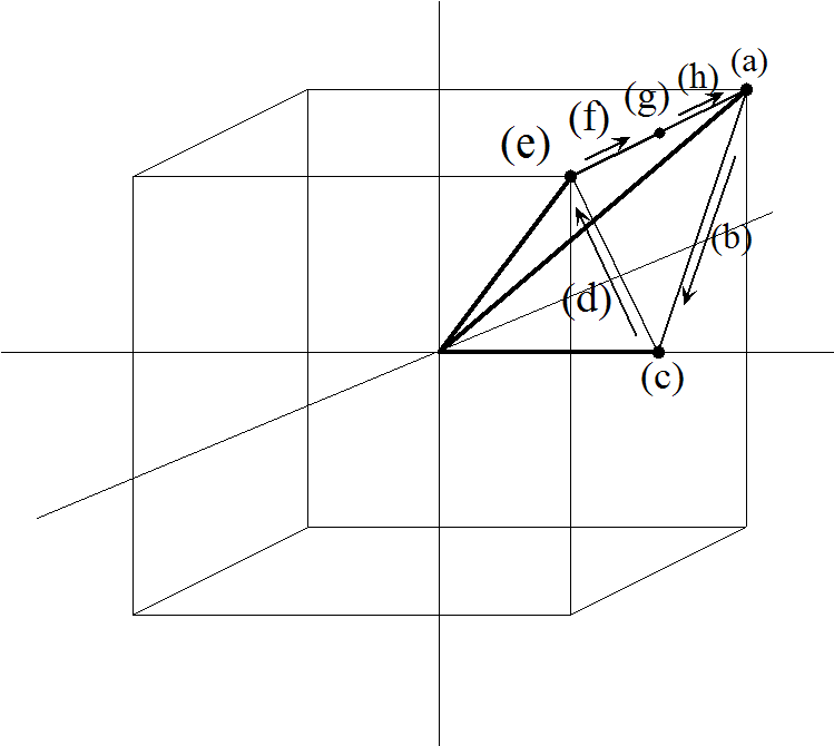
and the fundamental Weyl chamber is determined by the inequalities (see Figure 1):
| (3) |
The bounding cube on the figure helps to visualize the remaining 23 Weyl chambers in analogous positions. The Weyl group is generated by the reflections with respect to the walls of the Weyl chambers.
A generic adjoint (equivalently coadjoint) orbit, passing through an interior point of , is the real 12-dimensional manifold
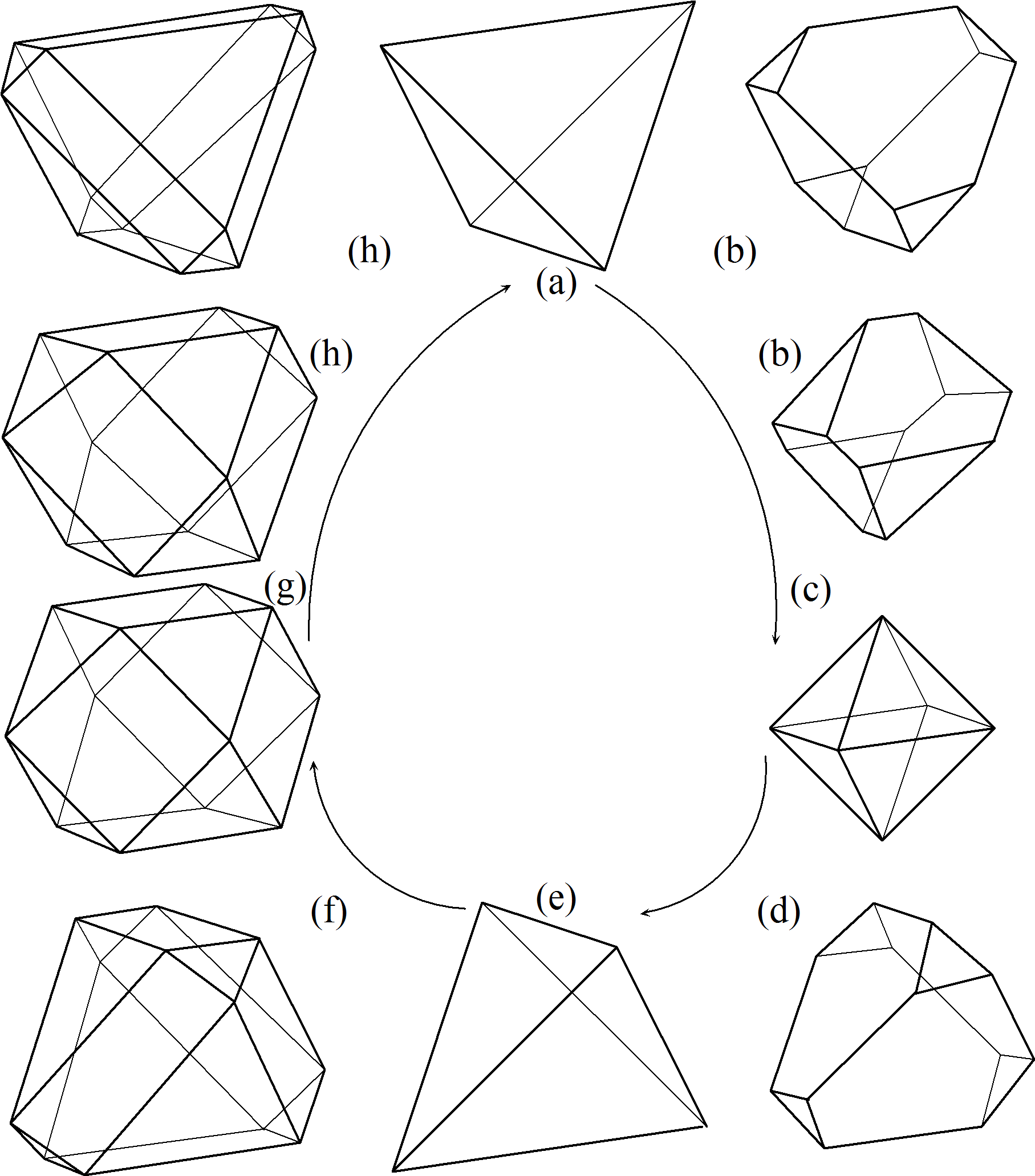
of “full” complex flags of . A point belonging to the faces or the edges of the closed fundamental Weyl chamber admits a stabilizer which contains properly the above torus subgroup, and so gives rise to a degenerate orbit. Points in with the corresponding stabilizer and orbit are listed in Table 1. We denote by and the unitary subgroups of associated respectively to the complex structures and on which act on a standard basis as follows:
| point in | stabilizer | orbit | image by | Fig. 2 |
| tetrahedron | (a) | |||
| tetrahedron | (e) | |||
| octahedron | (c) | |||
| truncated tetrahedron | (b) | |||
| truncated tetrahedron | (d) | |||
| skew-cuboctahedron | (h) | |||
| cuboctahedron | (g) | |||
| skew-cuboctahedron | (f) |
Table 1
The general theory (see [6]) leads us to distinguish three types of orbits. The “” orbits are the complex flag manifolds of where the total complex structure induces the canonical orientation on . The “” orbits are complex flag manifolds with a total complex structure inducing the opposite orientation on . A “” orbit is conjugate to a “” one by an element in exchanging the complex structure. Then we have the type orbits and which are partial complex flag manifolds. From this point of view, the -dimensional orbits reflect -inequivalent cases. However in the case under consideration, since , and are exactly the same group, the -type orbits are all identical.
The Weyl group of acts by permuting the coordinates and/or changing an even number of signs, so the Weyl orbit of in consists of itself and , ,. The resulting tetrahedron is denoted by . Analogously the Weyl orbit of is given by itself and the points , and , leading to . The specific position of a point in (Figure 1) determines in an analogous way the degeneracy of the Weyl orbit and hence the polytopes illustrated in Figure 2. Following the arrows 1–4 we see how the position inside affects the precise shape of the moment polytope. The image is determined by the non-degenerate Weyl orbit represented by the dodecahedron in the middle of Figure 4.
Obvious inclusion relations between the stabilizer groups listed in Table 1 show how the orbits are interrelated. We have the following differential fibrations with fibres for the and the projections and for the ’s. Again, as , both and contain the above .
| (4) |
Each fibre can be interpreted as a coadjoint orbit.
Proposition 1.
(Bernatska-Holod [5]) Given a compact semisimple Lie group , suppose that (the isotropy group of ) is not a maximal subgroup of . Then there exists a subgroup such that and fibres over with fibre .
We express this in symbols by .
Furthermore observe that the only orbit of is .
Then for , and .
The generic orbit fibres over the degenerate one:
| (6) |
But fibres over with fibre so:
| (7) |
The above fibrations are symplectic in the sense that their fibre is a symplectic manifold for which the transition mappings induce symplectomorphisms of . This is equivalent to a certain connection being flat [13]. More generally, for any compact Lie group , we have:
Proposition 2.
(Guillemin-Lerman-Sternberg [13]) Let be points in the same Weyl chamber. If the isotropy Lie algebras satisfy , then the map given by is a symplectic fibration with fibre a -coadjoint orbit.
In this context it is easy to prove that:
Proposition 3.
A fixed point of a given orbit fibres over a fixed point in a lower one.
This fact enables one to determine the image via of a fibre over fixed point in a lower orbit, i.e. the covex hull of fixed points contained in the fibre. Toric manifolds () can be recognized by their moment (Delzant) polytopes. We will provide several examples of how symplectic fibrations over (symplectic submanifolds of) coadjoint orbits are efficiently illustrated by the moment map, even though the torus actions are typically low-dimensional and thus not toric. For example the image of a generic orbit is a hexagon, and in Figure 3 we see how the symplectic fibration (6) is detected by the moment map. In fact, the -fibres over the fixed points in (vertices of the triangle) are mapped to segments anchored at the fixed points of the generic orbit. Analogous considerations enable us to capture graphically the essence of the symplectic fibrations (4) just comparing the moment polytopes as represented in Figure 4 and Figure 5. A more detailed explanation of this observation emerges in the context of Section 3, other examples are given in Section 4.
Remark 4.
Observe that is a subgroup of which suggests that fibres symplectically over with fibre (denote this projection by ). In contrast with Proposition 2 we cannot find a representative of the lower orbit and an element of the fibre over it in the same Weyl chamber. For example compare the stabilizers of and . We will return to this case in Section 4.


2 Riemannian geometry in six dimensions
Let be Lie groups, a subgroup of . It is a well known fact that a reduction of a -structure to an -structure can be realized by selecting a tensor , stabilized by in a suitable -module. The parameter space of such reductions is the -orbit of .
A section of the tensor bundle can be regarded as an endomorphism of each tangent space. Such an endomorphism can be analysed in terms of its kernel and other eigenspaces, which (as varies) give rise to distributions. Integrability properties of such distributions characterize the structure of .
Let be a Riemannian manifold of dimension . Any smooth -form determines a skew-symmetric endomorphism of each tangent space via
| (8) |
Suppose that is the largest non-trivial subgroup of which preserves at every point in . Then determines a reduction of the structure group to . There are many relevant examples of such a procedure. At one extreme (for N=2m) is the case when is an almost complex structure on (), the eigenspaces of are maximal complex isotropic subspaces of . If a -form is proportional to one associated to an almost complex structure, it determines an almost complex structure even though the corresponding is not an almost complex structure itself. In fact the eigenspaces of are again maximal complex isotropic subspaces of , and the eigenvalue is purely imaginary with respect to an underlying almost complex structure. At the other extreme if is a non-vanishing simple 2-form, then has dimension 2, and determines an almost complex structure on this subspace (). In these examples, satisfies
and thus induces an orthogonal transformation on . For the purposes of this article we say:
Definition 5.
Two distinguished Riemannian -structures defined via -forms are called compatible if the associated skew-symmetric endomorphisms commute.
The use of 2-forms to define a geometrical structure leads one naturally to consider coadjoint orbits for which are complex flag manifolds. An element of can be regarded as a skew-symmetric endomorphism. In even dimensions the eigenvalues of such an endomorphism are pure-imaginary and paired and its spectral structure is preserved by the orthogonal group. The flags in question are determined by the set of eigenspaces of and the stabilizer of the -form depends only on the set of eigenspaces and not on the precise eigenvalues.
In six dimensions . The torus (2) acts in the standard block-diagonal way. The images of the root spaces of are the subspaces , , . The Lie algebra is mapped to the -dimensional subspace of spanned by the elements (where ). Following this construction the image in of the fundamental Weyl chamber is generated by the elements
| (9) |
Every coadjoint orbit has a unique representative element in the closure thus:
Proposition 6.
Any -form at a point of an oriented Riemannian 6-manifold is equivalent under the action of to a linear combination with .
We can now introduce the Riemannian structure defined by a fixed 2-form. Such a structure is determined by a smooth section of the fibre bundle , where is a coadjoint orbit. The position of the representative of the orbit inside the image of determines the structure group of the reduction. Table 2, in which , are positive, relates positions inside to orbits ordered by dimension (recall Table 1).
Case -form SO(6) orbit 1 2 3 4 5 6 7 8 9
Table 2
We comment briefly case by case:
Case 1. The isotropy group is , so working pointwise, without implying integrability, we shall refer to the corresponding -structure as an orthogonal almost complex structures (OCS) on compatible with a fixed orientation. The parameter space at each point of is .
Case 2. parametrizes the OCS’s inducing the opposite orientation on .
Case 3 features the Grassmannian of oriented 2-planes in . A simple 2-form defines via (8) a splitting with an oriented 2-plane, and a 4-plane whose orientation is not specified. The orbit parametrizes a set of orthogonal almost product structures (OPS) studied by Naveira in [18] (alternatively defined by a -tensor field where and represent the projections on and on ).
Cases 4-8 are related to the 10-dimensional “intermediate” complex flag manifold; in this case the action is characterized by two distinct pairs of imaginary eigenvalues. The corresponding isotropy subgroup of is isomorphic to .
Definition 7.
Let be an -dimensional Riemannian manifold. A mixed structure (MS) on is a reduction of the structure group to , where .
Such a structure is equivalent to the simultaneous assignment of an OCS () and an OPS () which are compatible (). In our case and we set so that is the identity on the 2-plane.
Case 4. The -form belongs to the plane generated by and . The position of this point inside the Weyl chamber reflects the fact that is a linear combination of a 2-form arising from an almost complex structure and a simple 2-form arising from a positively-oriented -invariant 2-plane.
Proposition 8.
A orbit parametrizes MS’s determined by an OCS in and an OPS in whose 2-plane is -invariant and oriented consistently with .
Case 5 is analogous; parametrizes MS’s with and an OPS whose 2-plane is -invariant and oriented consistently with .
Cases 6 and 8. This time, the position of the 2-form in exhibits it as a weighted linear combination of two compatible OCS’s and .
Lemma 9.
If two OCS’s on are compatible then they coincide up to sign on a real -plane (and, therefore, on a complementary -plane).
Proof. Fix one of the structures, and use this to identify with . The second OCS lies in with respect to the first and its matrix has eigenvalues , whilst the first matrix is (say) times the identity. In particular, both matrices leave invariant a complex 2-dimensional subspace of , giving rise to a real 4-plane.∎
As and belong to different orbits, they coincide on an invariant -plane, but induce opposite orientations on the complementary -plane. In the specific case displayed, the latter is . Thus,
Proposition 10.
A orbit parametrizes MS’s determined by an OCS in and an OPS in whose 2-plane is oriented consistently with .
Case 7 is the special case in which the contributions of the two OCS’s have the same weight. The 2-dimensional subspace is determined by the kernel of and thus the orientation is not specified by the tensor. This corresponds exactly to Yano’s definition of Riemannian -structure [19, 20], further developed by Blair [7]:
Definition 11.
An -structure on a differentiable manifold is a tensor (as the one in (8)) satisfying , the existence of which is equivalent to a reduction of the structure group to .
In conclusion, the and type orbits parametrize at each point the -inequivalent (but -equivalent) mixed structures. The fact that -structures in six dimensions provide a special case of MS’s is due to the isomorphism (strictly speaking also the OPS’s parametrized by are examples of -structures).
Case 9 parametrizes the set of possible -reductions of the Riemannian structure, consisting of a choice of three orthogonal complementary -dimensional spaces in each tangent space.
Remark 12.
Our construction refines the description of a geometrical structures, in the sense that we put more emphasis on the defining tensor rather than merely the isotropy subgroup. However the stabilizer of the -form depends only on the spectral structure (set of eigenspaces) of the corresponding skew-symmetric endomorphism and does not depend on the specific eigenvalues. Thus all the points staying in analogous positions in represent the same -structure. The precise values of are not relevant.
In the case of OCS’s, OPS’s and f-structures we can identify the -structure with a real projective class in . All the points belonging to the same wall of represent the same MS.
3 Moment polytopes
Previously we analysed a coadjoint orbit as a symplectic manifold. The Riemannian -structures under consideration are now realized as smooth sections of fibre bundles with fibre . The mapping
which associates a -form to a specific -reduction can be interpreted (at each point of ) as the moment map
associated to the KKS symplectic structure. Combining this mapping we obtain the orthogonal projection which gives us the moment mapping
for the action of itself. To sum up,
Theorem 13.
The Hamiltonian action of the maximum torus of on associates a characteristic “moment polytope” to each of the Riemannian structures defined by a 2-form.
In Section 1 we proved, using standard Lie group theory, what the precise shape of the moment polytope associated to each structure is (compare Table 1 and Table 2). The aim of this section is to describe how those polytopes can be obtained and interpreted in terms of -forms and compatibility of -structures (in the sense of Definition 5). For this purpose the subsets of consisting of points fixed under the action of a suitable subgroup of the maximal torus provide in each orbit a “skeleton” of relevant structures. Those are the subsets on which is singular.
Let be a compact Lie group. Having chosen a maximal torus, we take a set of fundamental weights in . Denote by the set which includes the fundamental weights and all their conjugates, by the stabilizer group of each weight and by the Weyl group of the structure . Observe that is generated by the reflections induced by the roots orthogonal to . As leaves invariant , we have
where is the Lie algebra of . The previous equation can be read “backwards” to give , so the elements of subalgebra are preserved by the action of the circle subgroup
Theorem 14.
(Guillemin-Lerman-Sternberg [13]) The critical (or singular) sets of the torus moment map are the symplectic manifolds
The critical values of are the corresponding convex polytopes .
An immediate application of this theorem to the case of allows one to visualize the critical values of .
Proposition 15.
Given a vertex of the moment polytope of an -coadjoint orbit, the image by of the symplectic manifold consists of the intersection of with the plane orthogonal to , which passes through .
Figure 6 shows the directions of some roots orthogonal to and and the corresponding fixed-point sets. The roots generating and can be viewed as inward pointing normal vectors of the polytopes .

Remark 16.
The sets of points fixed by are -coadjoint orbits. The case of appears to be highly constrained in the sense that each critical set can be recognized by looking at its moment polytope. The fixed-point set of each carries an effective Hamiltonian action of a complementary subtorus in which is a maximal torus in . The stabilizer of is , its coadjoint orbits have been described in Section 1. Since is a toric variety, the filled triangles on Fig. 6 identify fixed-point sets symplectomorphic to . This implies that each filled hexagon represents necessarily a generic -orbit. The stabilizer of is . The symplectic manifolds and are coadjoint orbits of and both are toric varieties, mapped respectively onto the filled rectangles and the bold line segments on Fig. 6.
The sets of points fixed simultaneously by the action of two 1-tori are projected onto line segments determined as intersections of the images of the single 1-tori fixed-point sets. Examples of such projections are the edges of any polytope but also internal segments and segments contained in faces. Certain segments appear as images of sets invariant under . This fact is quite easy to justify in terms of sums of roots.
The Delzant Theorem [10] states that the toric moment map defines a bijective correspondence between symplectic toric manifolds and Delzant polytopes. The following Proposition gives an operative criterion for establishing whether a symplectic submanifold of a -coadjoint orbit is toric. The conditions on edges or vectors normal to faces, which define a Delzant polytope (simplicity, rationality and smoothness, see for example [9]) are related to a lattice in determined by the root system of .
Proposition 17.
Let be a compact Lie group with maximal torus , and let be the set of roots. Let be a coadjoint orbit of , and let be the moment map for the -action. Let be a connected -invariant symplectic submanifold and let denote the subset of points fixed by the torus action. Given a point define:
for some and .
If the vectors in are linearly independent for some , then is a symplectic toric manifold.
Proof. Since is connected, it is enough to prove that the weights for the -action on are linearly independent. Since , the weights for the action on are a subset of the weights for the -action on , which themselves are a subset of . So we only need to consider weights in . Given , let be the kernel of the character associated to . Then the isotropy submanifold must contain at least one fxed point such that is a positive multiple of .∎
The statement and the proof of Proposition 17 were suggested to the author by the reviewer of this article.
A relation to the theory of G-structures issues from the following (which is obvious):
Proposition 18.
If a -form is fixed by the action of some subgroup of the maximum torus , then the corresponding skew-symmetric endomorphism commutes with the action of on .
More concretely an OCS acts as a simultaneous rotation by on each of a triple of invariant -planes and can be interpreted as an element of a suitable one-torus. In particular, the OCS associated to acts as (see Figure 1). Similarly, the endomorphism determined by corresponds to .
We describe in this context the tetrahedra associated to both cases of almost complex structures. This technique will be very useful later on. The faces of each tetrahedron are projections of sets fixed by the action of the circle generated by the “opposite” fundamental weight, so they represent OCS’s commuting with the OCS represented by the opposite vertex.
Lemma 9 implies that two commuting OCS’s in the same orbit coincide on a -plane and differ by a sign on the complementary -plane. The sum of the corresponding -forms gives (twice) a simple -form detecting the common invariant and consistently-oriented -plane. We uniform the notation to the one of [1] setting (see (9)):
and will denote the corresponding OCS. The -forms in the orbit of , which define OCS’s commuting with are given by:
| (10) |
where and . The prototypes are the vertices of :
| (11) |
As is the projection to and
we have
Thus the projections of this form satisfy , and so lie in the plane passing through with . The planes perpendicular to each and passing trough the complementary vertices of the tetrahedron are obtained in the same way. Applying the same procedure to a generic -plane generated keeping the form inside , the Cauchy-Schwarz inequality leads to the condition (see [17]). Varying the vertex we get the entire set of inequalities that determine each of the tetrahedra.
Let us denote by (respectively ) the three-dimensional space of self-dual (anti self-dual) -forms on .
Lemma 19.
Given an OCS on , the set of -invariant and consistently-oriented planes is isomorphic to .
This is obvious because the set of complex lines in is . But to see the result in terms of 2-forms, recall that
A simple form can be written as a sum of elements in and of equal norm, and a -invariant simple -form is given by the expression
where and .
Corollary 20.
Given an OCS , the subset of of OCS’s compatible with , is in one-to-one correspondence with the set of -invariant -planes consistently oriented with .
Given an OCS on compatible with , there is an of common invariant planes oriented consistently with inside the common invariant -plane. It is easy to prove:
Corollary 21.
Given an OCS and an -invariant -plane oriented consistently with , there is an of OCS’s compatible with , for which is invariant and consistently oriented.
The edges of the tetrahedra (intersections of two faces) are projections of OCS’s commuting simultaneously with the two vertices opposite to the faces in question. Lemma 9 and Lemma 19 imply that these sets are -spheres. For example the edges which do not contain are projections of forms with fixed norm in:
| (12) |
In this context we can also determine the faces of the octahedron . Let be a vertex of or ; we can ask “what is the image in of the -invariant planes”. The octahedron combines the inequalities defining and ;
thus is obtained as an intersection of the tetrahedra as in Figure 7. This resumes the argument applied in [17] to determine . In the next section we will provide analogous interpretation of the moment polytopes related to the remaining coadjoint orbits.

4 A Klein correspondence
In Section 2, we introduced the symplectic fibrations of coadjoint orbits. Consider the lower part of the first and the third diagram in (4). The projections and (resp. , ) can be understood in terms of the classical Klein correspondence in which is identified with a non-degenerate quadric in :
1. parametrizes the projective lines in .
2. A point determines an -plane in , consisting of all the lines passing through that point.
3. A point determines a -plane in , consisting of all the lines lying in the plane .
In the light of our realization of coadjoint orbits as parameter spaces of Riemannian structures, this correspondence assumes a completely new interpretation. Namely,
Given a decomposition arising from an OPS , there is a worth of compatible OCS’s parametrized by . This is our projective line in .
Given an OCS we have the -invariant -planes generated by and each one determines an OPS.
Likewise, given an OCS we have the -invariant oppositely-oriented -planes generated by .
To understand , recall that the 2-sphere of unit self-dual forms parametrizes OCS’s on compatible with both metric and orientation. When combined with a standard almost complex structure on , we obtain a positively-oriented OCS on .
The results of Section 3 can be exploited to establish a mapping between moment polytopes induced by the Klein correspondence. A MS in determines an OCS , namely its projection via . This identifies the tangent space with , and -invariant splittings of are parametrized by complex 1-dimensional (or complementary 2-dimensional) subspaces in , i.e. by the projective space . Thus, the set of MS’s fibres over the set of compatible OCS’s with fibre .
The inverse image by of an OCS inside is determined by answering the question: “which are the OPS’s whose 2-plane is both -invariant and oriented consistently with ?” Working in terms of 2-forms, we take the non-degenerate 2-form associated to and add to it a simple -form representing the -invariant plane in question. For instance, can be easily determined by the technique introduced in Section 3, we see that belongs to the plane
| (13) |
In view of the results of Section 2 and the symplectic nature of the fibrations (recall Proposition 13), we conclude that the set of MS’s compatible with gets mapped by onto the triangular face of the truncated tetrahedron, generated by the vertices
| (14) |
This is a subset of of points fixed by . Lemma 19 gives the possibility to interpret the edges of this triangular face. For instance the edge joining the first two vertices in (14) is the projection of a set invariant under and . It represents the of -invariant and consistently oriented planes in the span . Figure 8 represents the map between polytopes induced by the maps and .

We can now test the mapping induced between polytopes on subsets of the lower orbits in the symplectic fibrations (4). Let be the OCS’s that correspond to the 2-forms in (11) i.e. the vertices in the tetrahedron . Adopting notation from [2], we call the edge joining the vertices and as in Figure 9.
Proposition 22.
Denote by . The image is the polytope shown on the left in Figure 9. The set is a symplectic toric manifold.
Proof. The coadjoint orbits of any compact classical Lie group admit a standard invariant complex structure defined by the action of a maximum torus on the root spaces of the isotropy representation (see [6]). The KKS form is the Kähler form of a canonical Kähler structure compatible with . The projections intertwine the complex structure. Therefore the preimage of a complex submanifold (observe that ) is a complex submanifold, and so it is a symplectic submanifold. For this reason, its moment image is the convex hull of its fixed points. Hence, one just needs to determine the fixed points which map to the desired set. But this is trivial as fixed points in the higher orbit belong to fibres over fixed points in the lower one. Now is -dimensional and is a real -dimensional symplectic manifold (a bundle over ), so is -invariant. Looking at , it is easy to check that the hypotheses of Proposition 17 are satisfied so is toric.∎
Remark 23.
Proposition 22 confirms that the mapping between polytopes arises from symplectic phenomena. Also in this case the moment map captures the essence of the symplectic fibration. The inverse image of each point of in is isomorphic to a , and the edge of the tetrahedron is the projection of a . The inverse image of the entire set is thus a symplectic -bundle over and the subset projects to “a triangle times a line”!
Analogously, the inverse image by of an element in is parametrized by suitably-oriented OCS’s on . Given an orthonormal basis of , we extend the -form by adding a unit element of or inside so as to obtain an OCS on . For example, can be completed to and in (recall (11)) and a whole 2-sphere of similar non-degenerate 2-forms. The same simple 2-form can be also completed to and in and an worth of OCS’s with the opposite orientation.
The proof of Proposition 22 holds in the following two cases.
Proposition 24.
Denote by the set of -planes in the subspace . The image is the rectangular prismoid represented in bold on the right of Figure 9. The set is a symplectic toric manifold.

Remark 25.
The image of by the moment map is the square intersection of with the plane . In the present context it should be interpreted as a projection of having -spheres respectively in and . We expect the subset of to be a symplectic bundle over . The intersection of with any plane orthogonal to is a rectangle, so this moment polytope is “a rectangle times a line”.
Proposition 26.
Let and denote the -invariant subsets of (both symplectomorphic to ) projected by on two disjoint faces of . The images are respectively a hexagon and a triangular prismoid as shown in Figure 10. The set is a symplectic toric manifold.

The sets represent -invariant planes. Both are symplectic fibrations over with fibre . The set contains the MS’s defined by itself (a projecting on the triangular face of on Fig. 10). The set of MS’s obtained by a plane in and the unique (by Corollary 20) corresponding OCS compatible with is a of MS’s compatible with , which projects on the internal triangle. Corollary 21 implies the fibre over each point of represents MS’s compatible with . This set projects on a hexagonal face of . Alternatively:
Remark 27.
The hexagonal face of represent MS’s determined by an OCS compatible with and a -invariant plane oriented consistently with . MS’s compatible with are parametrized by orbits, and the generic orbit is a symplectic bundle over .
The inverse image in of a point is given by all the forms obtained by adding to a “small” contribution negatively-oriented -invariant -plane. The inverse image of a in can be recovered replacing the positively-oriented -plane of the case with a negatively-oriented one. The map sends any OCS in in the corresponding of compatible OCS’s in and vice versa. This concludes our “-form interpretation” of the middle symplectic fibration in (4).
In Remark 4 we observed that should fibre over . This fact becomes obvious in view of Proposition 10. We can determine the inverse image of the point . This case requires a 2-plane that is invariant simultaneously by and . The subsets in invariant by the rotations generated by the roots corresponding to and project respectively onto the hexagons and in Figure 11. The projection of the inverse image of is the internal segment , remarkably it is obtained as the intersection of the above invariant sets. Now comparing Figure 11 and Figure 1 we see that there is no representative of the fibre in the Weyl chamber where stays.

The image of in consists of all the OCS’s for which this form represents the contribution of a negatively-oriented -invariant -plane (for example, full-rank forms involving ). It is easy to see that this set projects onto the edge . Keeping in mind Lemma 9 it should be not a surprise that the image of in projects onto the face in opposite to .
As another example, consider the form . Its image by is the midpoint of the segment . It can be interpreted as the sum of in and . The form maps to the midpoint of the edge .
We invite the reader to complete the analysis of the maps between the moment polytopes , and keeping in mind Proposition 10 and Remark 27. In particular analogous considerations enable one reader to interpret Figure 12.
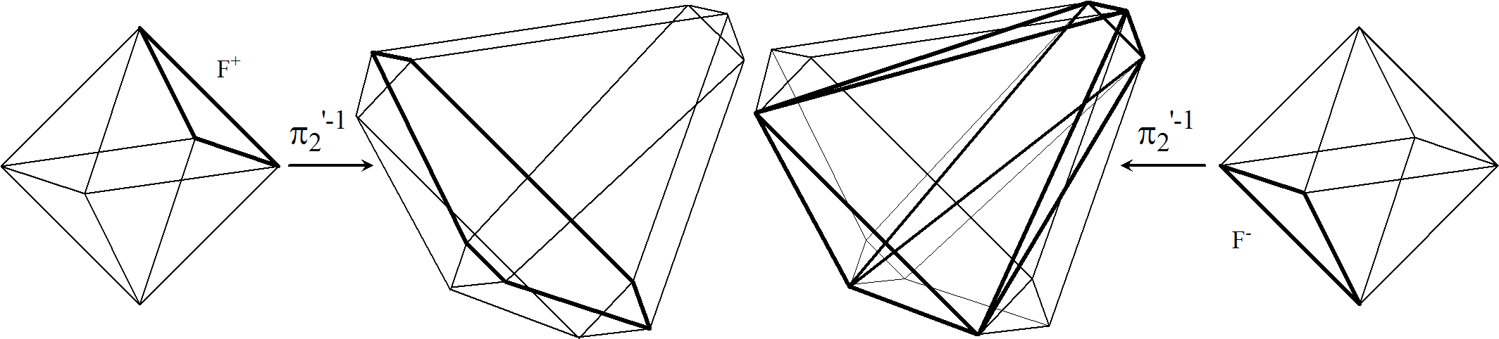
The moment polytope corresponding to (Figure 2g) is a special case of . The rectangular faces are squares. For the -structures, there is no way to define a map between moment polytopes corresponding to the symplectic fibrations in the middle diagram of (4). The lack of such a mapping is due to the degeneracy of the characteristic -form. In fact, in the case of the remaining orbits, there are two distinguished internal segments corresponding to the projections of the same -plane taken with two different orientations. In this case, the -form is not capable of determining the compatible orientation on its kernel. Graphically, this is expressed by the fact that the two segments (corresponding to the different orientations of the -dimensional kernel) intersect in the origin (see Figure 2(g) ). For example the form determines a splitting and can be extended to to yield a compatible OCS in . The image of by is the origin of , whereas the image of is the midpoint of an edge of the tetrahedron.
5 An application
The intrinsic torsion of a geometrical structure is the first order obstruction to its integrability. For this reason, a standard way of classifying Riemannian -structures is based on criteria whereby its intrinsic torsion tensor reduces to a specific subset of -irreducible components of the corresponding space of intrinsic torsion . For Riemannian -structures, is determined by the Levi-Civita derivative of the defining tensor and is isomorphic to , where is the orthogonal complement of the Lie algebra of in . The constraint can be stated requiring that some components of vanish, so we adopt the terminology null-torsion classes.
The prototype case gave rise to the sixteen classes of almost Hermitian manifolds à la Gray–Hervella [11]. The -irreducible components have also been described in [4] by complexifying the exterior algebra; the space is the complexification of a real vector space that is denoted . Denote by the irreducible complex -representations with dominant weight , and by the Hermitian complement of the image of under wedging with . We then have the following isomorphisms:
| (15) |
The irreducible components immediately above give rise to well known classes of almost Hermitian structures; lying in means that the structure is nearly-Kähler, – almost-Kähler, – cosymplectic Hermitian, – locally conformal Kähler etc. In particular, the component of in can be identified with the Nijenhuis tensor, and so Hermitian structures belong to the class .
Analogous classification of the OPS’s, developed by Naveira in [18] exploits the decomposition of the intrinsic torsion space
into the irreducible components
| (16) |
using the notation of Section 2.
We denote by and the spaces and , or the corresponding null-torsion classes.
In [16, 17] the same approach has been applied to MS’s. In six dimensions we exploit the geometrical interpretation of a -structure in terms of the underlying OPS and OCS. This allows the null-torsion classes of these MS’s to be described by means of the module
| (17) |
where in accordance with the notation introduced for (15). We shall also write , so that is a complex vector space of dimension 1 on which acts, and . Then can be shown to be isomorphic to the direct sum of 16 irreducible real summands:
| (18) |
(Tensor product signs are omitted, means . Also , and is the second symmetric power of .) The 10 non-isotypic summands have respective dimensions 4,2,6,2,2,2,2,6,6,2. This approach enables one to compare the intrinsic torsion of interrelated structures. For example, the fact that
| (19) |
implies the next result, also proved in [17].
Proposition 28.
The intrinsic torsion tensor of a MS is completely determined by the intrinsic torsion tensors of the underlying OCS and OPS. Conversely, determines the pair .
Recent work has focused on the problem of embedding classes of -structures on a parallelizable manifold inside an appropriate parameter space. In this case, one can consider -structures that stabilize a global section of some tensor power of the tangent bundle. Such structures are parametrized by a unique -orbit . The intrinsic torsion varieties (ITV’s) of a parallelizable manifold are the subsets of of structures belonging to the same null-torsion class (see [16, 17]). An analysis of ITV’s of structures on the Iwasawa manifold and other nilmanifolds has been carried out in [1, 2]. We highlight some relevant examples which we combine with the techniques of the present article.
The Iwasawa manifold is defined as the set of right cosets , where is the complex Heisenberg group and the natural lattice:
Nilmanifolds admit a natural parallelism determined by -left invariant vector fields. The complex -forms , and are left invariant on , and can be exploited for defining the following left invariant real -forms:
| (20) |
We will keep faithfully the notations of the previous sections referring to this basis of the cotangent spaces of . Setting being orthogonal we define on a standard Riemannian metric induced from a left-invariant tensor on (see [1]). Consider then the -structures obtained as reductions of this fixed Riemannian structure by stabilizing a -left invariant -form.
The following result has been proved as Theorem 1 in [1], though we can now give it a moment map interpretation.
Theorem 29.
(Abbena-Garbiero-Salamon) The set of invariant complex structures on is given by the disjoint union of the point and a . This is a -invariant subset of and its image by is the union of a vertex and the edge of .
A justification of the invariance of this set under the action of a maximal torus, based upon the fact that is a complex Lie group, is given in the author’s joint article [17], which also proves:
Theorem 30.
The ITV of OPS’s on the Iwasawa manifold characterized by an integrable 4-dimensional distribution (meaning ) is the complex submanifold
of whose image is the intersection .
Let us denote by the analogous subset of of OPS’s characterized by an integrable 2-dimensional distribution (meaning ). From [16] we know:
Theorem 31.
The subset of is the disjoint union of two -spheres consisting of the -invariant elements of . Its image by the moment map is
and is formed of two line segments.
The OPS’s in characterized by Theorem 30 are those for which a Nihenjuis-type tensor is zero [18], or equivalently those with vanishing component in (16). The corresponding null-torsion class of these foliations is therefore . A complete analysis of the ITV’s of OPS’s on the Iwasawa manifold is given in [15], as a result of which it turns out that
| (21) |
indeed it is easy to see that elements of have OPS torsion in . Moreover, elements of describe those OPS’s for which gives rise to a totally geodesic foliation and they are of class . Another result from [15] along these lines regards a relevant subset of :
Theorem 32.
The ITV of foliations of class on the Iwasawa manifold is the disjoint union of two ’s in . The OPS’s are characterized by the fact that their -plane is -invariant.
The two ’s in question are precisely the subsets previously denoted by and .
Knowledge of the fibrations of coadjoint orbits described in Section 1 enables us to detect ITV’s of mixed structures inside any 10-dimensional orbit (take for example in (4)). Consider an OCS and an OPS with intrinsic torsion in a known class. Proposition 28 implies that the points of in the intersection have pre-determined intrinsic torsion. If we consider in this way the inverse images of entire classes, their intersection determines a specific ITV of mixed structures inside . Theorem 29 and Theorem 30 now yield:
Corollary 33.
The ITV inside consisting of MS’s on of class is a disjoint union . It’s image by the moment map is shown in the centre of Figure 13.

Proof. By Proposition 24 is a real -dimensional symplectic toric manifold, has two disjoint components, a , and the symplectic toric manifold (recall Proposition 22). Proposition 17 implies that the -invariant subsets of and are real four-dimensional symplectic toric manifolds projecting on the faces of the corresponding moment polytopes, so the intersection of and is exactly the -invariant subset projecting onto the common rectangular face. This means . A dimensional check shows that the subsets of and simultaneously invariant under the action of two -s are all real two-dimensional symplectic manifolds, which project onto segments (edges of the polytopes), and are therefore toric manifolds symplectomorphic to . The intersection of and is a .∎
Corollary 34.
The ITV inside consisting of MS’s on of class is a disjoint union . The projection to consists of the segments , , in Figure 13.
Proof. This follows from Theorem 31, the proof is analogous to the previous-one. Proposition 17 implies that the trapezium faces of are projections of real four-dimensional -invariant symplectic toric manifolds ( bundles over ). ∎
Corollary 35.
The ITV inside consisting of MS’s on of class is a disjoint union . Its projection to consists of a line segment, a triangle and a trapezium as shown in the centre of Figure 14.

Proof. This follows from Theorem 32. The case of is analogous to the previous cases. The trapezium face of is the image of a -invariant toric submanifold ( bundle over ). Proposition 17 implies that this is a four-dimensional toric submanifold of .∎
Remark 36.
The -invariant (toric) submanifolds play a key role in the above results. Each corollary can be proved also in terms of -forms and compatibility of -structures. As an example we consider the intersection of and . Lemma 19 implies that the set of MS’s defined by an OCS in and an OPS in is a trivial bundle over . It follows from (12) that a generic -form in has the following expression
Without loss of generality, we can fix a unit -form . Let be an OCS in . Then
Adding a -form in to that of a consistently-oriented element in , we obtain a -form with component equal to . So is the intersection of with the plane , etc…
Remark 37.
The last three corollaries show that the intersections of ITV’s are determined by the intersections of their moment polytopes. Actually, it was the diagrams that led the author to formulate these results. They should lead to a similar description of the intrinsic torsion varieties for other structures on and on other nilmanifolds. The techniques developed in this article should help establish the extent to which these subsets of coadjoint orbits for are invariant by tori. Except for the graphical aspects, the methods are not restricted to the 6-dimensional case, but are perfectly general.
The Riemannian -structures that we have considered can also be obtained as reductions of spin structures, since is isomorphic to . Adopting a spinorial interpretation allows for the possibility of enlarging the theory to include structures not necessarily defined by a -form. An important example in six dimensions is that of -structures whose intrinsic torsion measures the extent to which a manifold fails to be Calabi–Yau. We refer the reader to [16].
Acknowledgements
This article is based on part of the author’s doctoral thesis [16], supervised by prof. Simon Salamon. The author thanks also the Geometriae Dedicata referee for the useful suggestions.
References
- [1] E. Abbena, S. Garbiero, and S. Salamon. Hermitian geometry on the Iwasawa manifold. Boll. Un. Mat. Ital., 11-B:231–249, 1997.
- [2] E. Abbena, S. Garbiero, and S. Salamon. Almost Hermitian geometry on six dimensional nilmanifolds. Ann. Sc. Norm. Sup., 30:147–170, 2001.
- [3] M. F. Atiyah. Convexity and commuting Hamiltonians. Bull. London Math. Soc., 14:1–15, 1982.
- [4] M. F. Atiyah, N. J. Hitchin, and I. M. Singer. Self-duality in four-dimensional Riemannian geometry. Proc. Roy. Soc. London, A 362:425–461, 1978.
- [5] J. Bernatska and P. Holod. Geometry and topology of coadjoint orbits of semisimple Lie groups. Proc. 9-th Internat. Conf. Geometry Integrability and Quantization Varna 2007, Softex:1–21, 2008.
- [6] A. L. Besse. Einstein Manifolds. Springer-Verlag, 1987.
- [7] D. E. Blair. Geometry of manifolds with structural group . J. Differential Geom., 4:155–167, 1970.
- [8] R. Bott. The geometry and representation theory of compact Lie groups. In Lecture notes Series 34 of London Mathematical Society. Cambridge University Press, 1979.
- [9] A. Cannas da Silva. Lectures on symplectic geometry. Lecture Notes in Mathematics 1764. Springer–Verlag, Berlin, 2001.
- [10] T. Delzant. Hamiltoniens périodiques et images convexes de l’application moment. Bull. Soc. Math. France, 116:315–339, 1988.
- [11] A. Gray and L. Hervella. The sixteen classes of almost Hermitian manifolds and their linear invariants. Ann. Mat. Pura Appl., 123:35–58, 1980.
- [12] V. Guillemin. Moment Maps and Combinatorial Invariants of Hamiltonian Space. Birkhauser, 1994.
- [13] V. Guillemin, E. Lerman, and S. Sternberg. Symplectic Fibrations and Multiplicity Diagrams. Cambridge University Press, 1996.
- [14] V. Guillemin and S. Sternberg. Symplectic Techniques in Physics. Cambridge University Press, 1990.
- [15] G. Mihaylov. Intrinsic torsion classes of Riemannian structures. to appear.
- [16] G. Mihaylov. Special Riemannian Structures in Six Dimensions. Doctoral thesis, University of Milan, 2008.
- [17] G. Mihaylov and S. Salamon. Intrinsic torsion varieries. Note di Matematica Universit� di Lecce, Suppl. N. 1, 2009. (Proc. Recent Advances in Diff. Geom. in honor of Kowalski, Lecce 2007).
- [18] A. M. Naveira. A classification of Riemannian almost-product manifolds. Rendiconti di Matematica Roma, 3:577–592, 1983.
- [19] K. Yano. On a structure defined by a tensor field of type satisfying . Tensor, 14:99–109, 1963.
- [20] K. Yano and M. Kon. Structures on Manifolds. World Scientific Publishing, 1984.