Shell Model in the Complex Energy Plane

Antibound (or virtual) states lie on the negative semi-axis of the imaginary $k$: $k_{n}=-i\kappa_{n}$  ($\kappa_{n}>0$) (see Fig. 2). They have real and negative energies that are located in the second Riemann sheet of the complex energy plane [40, 41, 42, 43]. Asymptotically, the radial wave function of a virtual state grows exponentially:

$$w_{n}(E_{n},r)\sim O_{l}(k_{n}r)\sim e^{ik_{n}r}=e^{\kappa_{n}r}.$$

(7)

As often discussed in the literature, it is difficult to provide a physical interpretation to virtual states. In the Hilbert space formulation of quantum mechanics, a virtual state is not considered as a state but as a feature of the system (as the second energy sheet is considered unphysical and inaccessible through direct experiments). In the RHS formulation, the virtual state can be interpreted both as a vector in the RHS and as a pole of the $S$-matrix. The latter implies that virtual states can be “seen” only close to the threshold; they manifest themselves in an increased localization of low-energy scattering states. Consequently, the presence of a virtual state at a sufficiently small energy has an appreciable influence on the scattering length and the low energy scattering cross section. Classic examples include the low-energy $\ell$=0 nucleon-nucleon scattering characterized by a large and negative scattering length [42, 44]. Related to this is an increased localization of real-energy scattering states just above threshold [45].

It is instructive to study the energies of antibound states as a function of potential parameters. A detailed study of this problem was done by Nussenzveig [46] (see also Ref. [47] for a discussion of the one-dimensional case). To this end, it is convenient to fix the geometry (radius and diffuseness) of the potential and follow the trajectories of the bound and antibound poles as a function of the well depth $V_{0}>0$. If there is no potential barrier, e.g., for $s$-wave neutrons, no narrow resonances appear. Here, by increasing $V_{0}$ from the minimal value at which the antibound state appears, the pole goes across $k=0$, forming a bound state with a radial wave function having one node, $n=1$. For protons or for $l>0$ neutrons, a potential barrier is present which can support resonant poles. In this case, decaying and capturing poles appear in pairs which move towards the imaginary $k$-axis as $V_{0}$ increases. At certain values of $V_{0}$ the poles meet at $k$=0, forming a double singularity. For still larger values of $V_{0}$, one of the poles becomes a bound state, while the other one moves down as an antibound state.

Neutron $l$=0 pole trajectories are shown in Fig. 3 as a function of $V_{0}$ for a square well potential. The behavior of the antibound poles conforms to the general pattern discussed above. Namely, below $V_{0}=1.05$ MeV, there appears only one antibound state. This pole moves to the upper half $k$-plane and forms a bound state with one node. By increasing the depth further from $V_{0}=9.05$ MeV, there appear two antibound poles. One of them moves upwards and at about $V_{0}=9.5$ MeV, it emerges as a $2s$ bound state, while the other one moves down and remains antibound. At about $V_{0}=26$ MeV three antibound and two bound states are present. By increasing $V_{0}$ to 30 MeV, the antibound pole lying closest to the origin becomes bound, resulting in three bound and two antibound states. At $V_{0}$=30 MeV, the $3s$ bound state is closer to the origin than the corresponding antibound pole. Therefore, there are no antibound poles between the loosest bound state and the threshold [40]. For the cases with a non-zero barrier, the resonant poles meet in the origin and one obtains a similar pattern as in Fig. (3) but with the Im($k$)-axis shifted down by about $k=0.15$ fm^-1. This shift would change the relative distance of the antibound and bound states with respect to the origin, with one antibound pole to appear between the loosest bound state and the threshold [40].

In the original formulation of the completeness relation (6), only decaying poles with

$$arg(k_{n})>-{\pi\over 4},\quad\quad Re(E_{n})>0$$

(8)

were considered. Consequently, virtual resonances (resonant poles with $Re(E_{n})<0$) and antibound states were excluded from the Berggren ensemble. The Berggren representation has been generalized in Ref. [48] by including a virtual state into the discrete part of the basis. The generalization requires a slight deformation of $L^{+}$ as indicated in Fig. 2. More recently, this generalized Berggren representation was used in a full form (i.e., including the scattering component) for the description of drip-line nuclei ¹¹Li and ⁷²Ca [49, 50]. A large destructive interference between the virtual state and the scattering contour states has been observed. In this picture, the bound ground state of ¹¹Li could be explained in terms of unbound states of ¹⁰Li. Soon afterwards it was noted [51] that a generalized Berggren basis is not optimal as far as the number of basis states is concerned. Indeed, as the halo wave function has a decaying character at large distances due to the exponentially increasing asymptotics of the virtual state (7), its inclusion in the basis always induces strong negative interference with the scattering states. Therefore, adding antibound states to the basis is not beneficial in GSM applications, as more discretized scattering states are necessary to reach a required precision.

The completeness relation by Berggren (6) can be derived from the Newton completeness relation for the set of real-energy eigenstates of a short-range potential [40]:

$\displaystyle\sum_{n\in(b)}|u_{n}\rangle\langle u_{n}|+\int_{0}^{+\infty}|u(k)\rangle\langle u(k)|dk=1.$

(9)

The proof can be carried out by deforming the real momentum axis associated with positive-energy scattering states into the $L^{+}$ contour of Fig. 2 and applying the Cauchy integral theorem [14]. This is possible because resonant states appear as residues, due to their $S$-matrix pole character.

Bound and real-energy scattering states generated by a potential bearing a Coulomb tail naturally form a complete set as well, as all self-adjoint operators possess a spectral decomposition [52]. However, methods used in Ref. [52], relying on the Lebesgue measure theory, are very general and fairly abstract. Thus, a simple demonstration of the completeness relation for potentials with a pure Coulomb asymptotic behavior is called for. The proof of (9) relies on the analyticity of the Green’s function of a local potential that is integrable for $r\rightarrow+\infty$ [40]. Potentials having a Coulomb tail, proportional to $r^{-1}$, have not been considered in Ref. [40]. Moreover, non-locality often appears in practical applications [53], so it is important to demonstrate the completeness relation for non-local potentials having a Coulomb asymptotic behavior. This has been done recently in Refs. [53, 54], where detailed derivations can be found.

In short, the main assumption behind the proof presented in Refs. [53, 54] is that beyond a finite radius $R_{0}$ the potential behaves as $r^{-1}$. The corresponding radial Schrödinger equation reads:

$\displaystyle u^{\prime\prime}(k,r)=\left(\frac{\ell(\ell+1)}{r^{2}}+v(r)-k^{2}\right)u(k,r)+\int_{0}^{R_{0}}w(r,r^{\prime})~u(k,r^{\prime})~dr^{\prime},$

(10)

where $v(r)$ and $w(r,r^{\prime})$ are respectively the local and non-local potentials. For $r>R_{0}$, the wave function is a linear combination of regular and irregular Coulomb functions. Their analytical character and the fact that regular Coulomb wave functions form a complete set [54, 55, 56] are important to the demonstration of the completeness. Using analytic continuation arguments, one can also demonstrate that the set of bound and real-energy scattering states generated by complex potentials $v(r)$ and $w(r,r^{\prime})$ is complete, provided no exceptional points, i.e., bound states of norm zero [57], are present.

Heuristic methods often precede a complete formulation of the physical theory in terms of an adequate mathematical apparatus. This was the case for Dirac’s formulation of quantum mechanics [58] which a posteriori found a satisfactory setting in the RHS [9, 10]. This is also the case for theoretical developments utilizing Gamow states to describe weakly bound and/or unbound states of quantum systems. The Berggren completeness relation [32], which replaces the real-energy scattering states by the resonance contribution and a background of complex-energy continuum states, puts the resonance part of the spectrum on the same footing as the bound and scattering spectrum. However, resonances do not belong to the usual Hilbert space, so the mathematical apparatus of quantum mechanics in Hilbert space is inappropriate and cannot encompass concepts such as Gamow states. Quite unexpectedly, it turned out that the mathematical structure of the RHS is ready to extend the domain of quantum mechanics into the time-asymmetric processes such as decays.

The RHS, or Gel’fand triple, is a triad of spaces [5, 6, 59]:

$\displaystyle\Phi\subset{\cal H}\subset\Phi^{\times},$

(11)

which represent different completions of the same infinitely dimensional linear space $\Psi$. $\Phi$ (the subspace of test functions) is a dense subspace of Hilbert space ${\cal H}$, and $\Phi^{\times}$ (the space of distributions) is the space of antilinear functionals over $\Phi$. $\Phi$ is also the largest subspace of ${\cal H}$ on which expectation values, uncertainties and commutation relations can be correctly defined for unbounded operators.

The linear functionals over $\Phi$ are contained in the space $\Phi^{{}^{\prime}}$ which is related to another RHS:

$\displaystyle\Phi\subset{\cal H}\subset\Phi^{{}^{\prime}}~~.$

(12)

One should stress that ${\cal H}$ in (11) and (12) does not have any particular significance in the RHS formalism. For all physics problems, one needs only the dual pair of spaces $\Phi\subset\Phi^{\times}$ which characterize the considered quantum system. For example, bras and kets, which are related to the continuous part of the spectrum of an observable, belong to $\Phi^{{}^{\prime}}$ and $\Phi^{\times}$, respectively, and not to ${\cal H}$. Apparently, the RHS provides also a more convenient framework than ${\cal H}$ to capture physical principles of quantum mechanics. The Heisenberg’s uncertainty relations are properly defined on $\Phi$, and not on ${\cal H}$.

Besides implementation of Dirac’s formalism of bras and kets, the RHS provides a framework for a quantum mechanical description of common irreversible processes, like the formation or decay of quantum states. Indeed, $\Phi^{\times}$ may contain generalized eigenvectors of the observable(s) with complex eigenvalues. The generalized eigenvectors of the Hermitian Hamiltonian are Gamow vectors. Examples of the RHS for the observables having a continuous part in the spectrum can be found, for example, in Refs. [60, 22].

Gamow vectors are state vectors of resonances. They belong to RHS and not to ${\cal H}$ since the self-adjoint operators in ${\cal H}$ can only have real eigenvalues. Like the plane waves (the Dirac kets), the Gamow functions are not square integrable and must be treated as distributions. In this way, one succeeds to generate Gamow bras and kets which fit naturally in the RHS. However, unlike the Dirac kets, the probability density for Gamow functions is not constant but increases exponentially in space.

Rules for the normalization of Gamow functions and corresponding completeness relations have been proposed [34, 32, 35, 61, 62, 39] independently of the RHS formulation. Similarly, the momentum space representation for Gamow functions has been introduced [63, 64]. RHS offers a mathematical framework to formulate those results rigorously. In particular, the RHS provides a unifying dual description of bound, resonant and scattering states both in terms of the $S$-matrix and in terms of the vector in the RHS. The transition amplitude ${\cal A}(E_{n}\rightarrow E)$ from a resonance of energy $E_{n}$ to a scattering state at an energy $E$ ($E\geq 0$)[22]:

$\displaystyle{\cal A}(E_{n}\rightarrow E)=i\sqrt{2\pi}N_{n}\delta(E-E_{n}),$

(13)

where $N_{n}$ denotes the normalization factor, is proportional to the complex $\delta$-function [65] which, far off the threshold energy in the region of the resonance, can be approximated by the Breit-Wigner amplitude. This physically expected result provides a formal link between Gamow states and nearly-Lorentzian peaks in cross-sections for narrow, isolated resonances.

Interpretation of certain aspects of the RHS formulation of quantum mechanics is still debated, and connections between Berggren and RHS formulations continue to be studied (for a recent review, see [60]). One aspect of this discussion concerns complex matrix elements of the operators and probabilistic interpretation of the resonant wave function. As an illustration of this problem for resonances, let us consider the solution of the Schrödinger equation $\chi(\mathbf{r},t)$ for a s.p. Hamiltonian $\hat{h}$:

$\displaystyle i\hbar{\partial\over{\partial t}}\chi(\mathbf{r},t)={\hat{h}}\chi(\mathbf{r},t).$

(14)

In the stationary picture, the resonant wave function is the product of time-dependent $\tau(t)$ and space-dependent $\psi(\mathbf{r})$ factors:

$\displaystyle\chi(\mathbf{r},t)=\tau(t)\psi(\mathbf{r}),$

(15)

where the time-dependent factor is:

$\displaystyle\tau(t)=e^{-i{{\tilde{E}_{n}}\over\hbar}t}.$

(16)

The complex energy $\tilde{E}_{n}$ (1) is the generalized eigenvalue of $\hat{h}$ with the complex wave number $k_{n}$ (3). The corresponding space-dependent eigenfunction $\psi(\mathbf{r},k_{n})$,

$$\psi_{n}=\psi_{n{\ell}jm}(\mathbf{r},k_{n})={u_{n{\ell}j}(k_{n},r)\over r}\bigl[Y_{\ell}(\hat{r})\chi_{s}\bigr]_{jm},$$

(17)

satisfies an outgoing wave boundary condition. At large distances, the radial part of the $\ell$=0 wave function is proportional to $\exp(ik_{n}r)$. For a decaying resonance, $k_{n}=\gamma_{n}-i\kappa_{n}$ ($\gamma_{n},\kappa_{n}>0$), the time-dependent factor

$\displaystyle\tau(t)=e^{-i{{\tilde{E}_{n}}\over\hbar}t}=e^{-i{{E_{n}}\over\hbar}t}e^{-{\Gamma_{n}\over{2\hbar}}t}~~,$

(18)

describes an exponential decay with a decay width $\Gamma_{n}$. As $r$ increases, the radial part of $\psi(\mathbf{r},k_{n})$ oscillates with an exponentially growing amplitude:

$\displaystyle e^{ik_{n}r}=e^{i\gamma_{n}r}e^{\kappa_{n}r}=[\cos(\gamma_{n}r)+i\sin(\gamma_{n}r)]e^{\kappa_{n}r}~~.$

(19)

The decay process in this picture is unlimited in both time ($t\in[0,\infty]$) and space ($r\in[0,\infty]$) and, henceforth, continues forever. This feature guarantees, in fact, the particle-number conservation [66]: the exponential temporal decrease of the wave function amplitude is complemented by its exponential spatial increase, and the divergence of the resonance wave function assures that the particle number is conserved.

In general, the quasi-stationary description of a time-dependent physical process works well when the decaying state is narrow, as in this case the formation of a state and its subsequent decay can be well separated in time. A narrow Gamow resonance has a large overlap with a properly shaped wave packet [67] and its radial wave function is similar to a bound state wave function while the imaginary part is small inside the nucleus. In the reaction cross section, such a narrow resonance shows up as a sharp peak which can be well separated from the non-resonant background.

Another aspect of the debate on the physical interpretation of Gamow vectors concerns the expectation value of an operator in a resonant state. Berggren’s interpretation of real and imaginary parts of the expectation value of an operator is based on the discussion of interference effects in the reaction cross-sections [68]. Berggren showed that the imaginary part of the complex cross section calculated with the Gamow resonance as a final state describes the interference of that resonance with the non-resonant background. In a later paper [69], Berggren demonstrated that for any operator which commutes with the Hamiltonian, the expectation value of that operator is the real part of its matrix element, and the negative of the square of the imaginary part of the matrix element can be associated with the square of an uncertainty of the expectation value. This proof holds only for operators which commute with the Hamiltonian. It turns out that the Berggren interpretation of the expectation value [69] is largely equivalent to the RHS formulation by Bohm and Gadella [70] and coincides with it in the leading order [15, 71].

The meaning of a complex radial expectation value was studied in Ref. [72] using a model of two coupled channels [73]. It was found that the radial expectation value in this model can be interpreted according to Berggren’s prescription and that it can be used to characterize the resonances as long as the wavelength of the decaying wave is shorter than the radial extension of the resonant state.

Already in 1970, in the pioneering work employing resonant states, a truncated resonant basis composed of bound neutron and resonant proton states was used to describe isobaric analog resonances [37]. The pole expansion of the radial wave function, the Green’s function, and the scattering matrix were subsequently discussed in a rigorous way in Ref. [74] by using the Mittag-Leffler (ML) expansion. They used the normalization of the pole solutions introduced in [34] and later employed in, e.g., Refs. [61, 75]. The authors of Ref. [74] suggested that the pole expansion could be used in (shell-model-type) nuclear structure calculations; however, they worried about the non-orthogonality of the basis. In a numerical study [76], the usefulness of the ML-type pole expansion of the Green’s function was examined. The question of overcompleteness was finally put to rest by Berggren and Lind [77].

Resonant state expansions were also used by atomic physicists for calculating the $S$-matrix, expressed as a sum of pole terms and a contour integral [78]. The positions of the poles were calculated by using the uniform complex scaling (see Sec. 3), while the residues were obtained by using numerical methods described in Refs. [79, 80]. Neutron emission from a heavy-ion reaction was modeled in a time-dependent two-center shell model in Ref. [81]. Therein, resonant states were calculated in the momentum space using the potential separable expansion (PSE) method [82, 83], in which the potential is expanded in a square integrable (harmonic oscillator; HO) basis, and the proper asymptotic of the wave function is guaranteed by the presence of the free Green’s function.

A less severe truncation of the Berggren basis was employed in the late 1980s in the resonant approach to the random phase approximation (RRPA), in which the contribution from the non-resonant continuum was neglected [84, 85]. Such an expansion is usually referred to as a pole approximation. (A detailed summary of the early theoretical approaches employing resonant states can be found in Ref. [86].) A similar pole approximation was used in the RRPA description of giant resonance escape widths [87]. A careful test of different pole expansions was carried out in Ref. [76] by using a benchmark continuum RPA result for the particle-hole response function (see Sec. 2.6 for details). It was found that the ML-type pole expansion was closer to the continuum RPA, based on the Green’s function, than the pole approximation. This result was explained by Berggren and Lind [77] who identified the ML-type pole expansion of the resolvent by using the so-called $U$ contour (see Fig. 2) in the complex $k$-plane. Unfortunately, an expansion using the $U$ contour,

$$1={1\over 2}\sum_{i=a,b,c,d}|u_{i}\rangle\langle\tilde{u}_{i}|+{{1}\over{\pi}}\int_{U}|u(k)\rangle dk\langle u(k^{*})|,$$

(20)

cannot be used in shell-model-like calculations because the factor $1/2$ in the front of the sum over the resonant (bound, antibound, capturing, and decaying) states destroys the idempotency of the unity operator [88]. In addition, pole expansions of type (20) are accurate only if very many poles (up to some large energy cut-off) are included in the sum; contributions from broad and virtual resonances (having negative real energies) are in fact essential [88].

In Ref. [89], Gamow states were expanded in a finite $r\in[0,R_{o}]$ interval by using a finite number of square integrable basis states, called Siegert pseudostates (SPS). The expansion coefficients were determined by solving a normal eigenvalue problem where the dimension of the system has been doubled. This doubled system represents an eigenvalue problem with a weight matrix of the Bloch operator. The weight matrix allows the continuation of the SPS into the tail region and defines a special inner product in which a completeness relation can be constructed for the SPS. A pole expansion of the Green’s function, similar to the ML expansion of Ref. [88], was carried out. This expansion was further exploited in Ref. [90]. The usefulness of SPS was further demonstrated in studies of time evolution of an infinitely extended system [91].

The resonant and continuum components of the strength function were calculated by using the Berggren completeness relation in studies of Coulomb breakup of ¹¹Be [92]. They found the non-resonant contribution of the part of the contour which returns to the real $k$-axis negligible. A similar result was obtained in Ref. [93].

In some of the pole expansions mentioned above, complex eigenvalues and radial wave functions of resonant states were calculated using the code gamow [94]. Later, more efficient numerical techniques have been used based on the piecewise perturbation method [95, 96]. In other work [97] spherical resonant states were obtained by solving a non-linear set of equations. Bound and resonant state energies were calculated in code pseudo by using the PSE method in [98] for an axially symmetric potential by finding the zeroes of the Fredholm determinant of the Lippmann-Schwinger equation. Recently a method was developed in which the momentum-space Schrödinger equation was solved by a contour deformation method [93].

More recent applications of pole expansions include a description of giant multipole resonances [99] (see Sec. 2.6), and partial decay widths corresponding to the proton decay from the Gamow-Teller and isobaric analog state resonances [100]. The Berggren representation in its full form, including the complex scattering continuum, was employed in Ref. [101] to describe the eigenstates of a realistic one-body nuclear Hamiltonian. In this work, eigenstates of a spherical symmetric potential were expanded in a full Berggren basis of a different potential. (Examples of such expansions are presented in Sec. 4.5.) The full Berggren ensemble was employed in studies of the average s.p. level density [102] and shell corrections [103, 104]. Quasiparticle resonances can be constructed from the Gamow resonances in the BCS approximation by generalizing the standard BCS to the complex energy plane if the contour integral is neglected. If the non-resonant contribution is included, the contribution from the continuum level density has to be added [105] when calculating the particle number. However, a proper description of pairing correlations in weakly bound systems must go beyond the BCS approximation [106]. Here, the tool of choice is the Gamow-HFB method to be mentioned in Sec 4.4.

Gamow states and resonant expansions have been extensively used in the description of alpha, proton, and neutron emission from nuclei. For very narrow alpha and proton resonances, a single-channel Gamow approximation that ignores the non-resonant background is fully adequate [107, 108]. An attempt was made to calculate resonant states of a deformed potential by means of an expansion in a spherical Berggren basis [109, 110]. However, for a description of narrow proton resonances in deformed nuclei, the accuracy of spherical expansion turned out to be not satisfactory and alternative approaches were used. One of them was the direct numerical integration of the set of coupled differential equations using the piecewise perturbation method. The resulting code ccgamow was employed in Ref. [111] to explain full and partial decay widths of protons from axially symmetric nuclei within an adiabatic approach that ignores the rotational excitations of the daughter system. A full non-adiabatic description of proton emitters was carried out in Refs. [112, 113] using a modified version of the coupled channels program nonadi, and the extension to the triaxial case can be found in Ref. [114]. A shell-model analysis of the proton emission from ³¹Cl using Gamow wave functions was performed in Ref. [115]. In a study of Ref. [116], Gamow states were used to benchmark a modified two-potential approach to tunneling problems.

The applications of resonant states mentioned so far were concerned with the s.p. space. By 2003, however, it became possible to apply the Berggren ensemble to a general many-body case. In two parallel studies [117, 118], based on a configuration mixing approach employing the one-body Berggren ensemble, two-particle resonances in ⁸⁰Ni and ¹⁰²Te were calculated using separable multipole interactions [117], and systematic calculations for the neutron-rich nuclei ^6-10He and ^18-22O were carried out using the surface-delta interaction [119]. More applications soon followed (see Sec. 6). In the following, we shall refer to these two realizations of the SM in the complex energy plane as the Gamow Shell Model since the underlying concept is the same.

Continuum RPA (CRPA) is a useful tool for testing the usefulness and accuracy of resonant state expansions. For separable multipole-multipole interactions, the solution of the CRPA equations is obtained by finding complex roots of the corresponding dispersion relation [76, 99]. Complex energy poles of the particle-hole response $R(E)$ yield positions and full widths of the correlated resonances while the partial decay widths of these states can be obtained from the associated residua.

Within CRPA, the particle Green’s function in a selected partial wave is

$$g(r,r^{\prime},k)=-{{u(k,r_{<})~v(k,r_{>})}\over{W(u,v)}},$$

(21)

where $W$ denotes the Wronskian of the regular $u(k,r)$ and irregular $v(k,r)$ solutions at $r_{<}$=$\min(r,r^{\prime})$ and $r_{>}$=$\max(r,r^{\prime})$, respectively, at real values of $k$. In the standard Berggren expansion using the $L$ contour of Fig. 2, the corresponding Green’s function can be written as:

$$g_{L}(r,r^{\prime},k)=\sum_{i=b,d}{{u_{i}(k_{i},r)~u_{i}(k_{i},r^{\prime})}\over{k^{2}-k_{i}^{2}}}+{1\over\pi}\int_{L}{{u(q,r)u(q,r^{\prime})}\over{q(k-q)}}dq.$$

(22)

On the other hand, if one uses the $U$ contour of Fig. 2, the Green’s function takes the form:

$$g_{U}(r,r^{\prime},k)=\sum_{i=a,b,d,c}{{u_{i}(k_{i},r)~u_{i}(k_{i},r^{\prime})}\over{2k_{i}(k-k_{i}})}+{1\over\pi}\int_{U}{{u(q,r)u(q,r^{\prime})}\over{q(k-q)}}dq~.$$

(23)

The two complex-energy representations of Green’s function given by Eqs. (22,23) and the real-energy expression (21) are mathematically equivalent; hence, they should give the same results in practical applications.

From a practical point of view, it is interesting to know if one can choose the complex contours in such a way that the contributions from the integrals in Eqs. (22) and (23) become negligible. This has been checked in Ref. [76], in which the particle-hole response functions were calculated for a square-well potential supplemented by the Coulomb field. For narrow and isolated resonances, the partial widths obtained by using the leading pole term in Eqs. (22) and (23) agree with the exact result within 10 %. The subsequent calculations of Refs. [88, 99] using the Woods-Saxon potential demonstrated that the contribution from the $U$ contour to the p-h response function could be further reduced but this does not hold for the $L$ contour. Furthermore, it was shown [77, 14] that neglecting the integral in Eq. (22) destroys the symmetry of the resolvent and causes an artificial threshold behavior of the Green’s function.

The isobaric analogue resonance (IAR) can be described phenomenologically by the coupled-channel Lane equations (CCLE) [4]. The IAR-CCLE problem offers an excellent opportunity to compare the complex-energy GSM approach with the standard CCLE solution along the real energy axis. Such a test has been carried out in Ref. [120] for the Lane Hamiltonian. Within CCLE, the multichannel Schrödinger equation has been solved by a direct numerical integration. The resulting proton scattering $S$-matrix has been calculated along the real energy axis in the region of the IAR and then fitted by using a single pole approximation,

$$S(E_{p})=e^{2i\delta_{p}(E_{p})}\left(1-i\frac{\Gamma}{E_{p}-\cal{E}_{IAR}}\right),$$

(24)

to determine the position $E_{r}$ and width $\Gamma$ of the IAR. In Eq. (24), the background phase shift $\delta_{p}(E_{p})$ was assumed to have a linear energy dependence in order to better reproduce the non-resonant background. The best fit parameter values, denoted by $E_{r}(CCLE)$ and $\Gamma(CCLE)$, are listed in Table 1. They coincide with the GSM eigenvalue ${\cal E}_{IAR}=E_{r}(GSM)-i{\frac{\Gamma(GSM)}{2}}$ within $1$ keV even for the broad states.

The integrated effect of the proton continuum along the complex path is small but essential to yield the correct value of $\Gamma(GSM)$.

The radial s.p. wave functions $u(k,r)$ that enter the Berggren ensemble (6) are solutions of the radial Schrödinger equation:

$\displaystyle\frac{d^{2}u(k,r)}{dr^{2}}=\left(\frac{\ell(\ell+1)}{r^{2}}+\frac{2m}{\hbar^{2}}V(r)-k^{2}\right)u(k,r),$

(30)

where $\ell$ is the orbital angular momentum, $m$ is the reduced mass of the nucleon, and $V(r)$ is the one-body potential that generates the basis. The choice of the potential is in principle arbitrary, but in practice, one is trying to optimize it by adjusting its parameters to experimental s.p. states. Another option to calculate it is using the Hartree-Fock (HF) method, as discussed in Sec. 4.4.

In many applications, a Woods-Saxon (WS) central field is used, supplemented by the spin-orbit and Coulomb potentials:

$$V(r)=-V_{0}f(r)-4V_{so}(\mathbf{l\cdot s})\frac{1}{r}\left|\frac{df(r)}{dr}\right|+V_{c}(r),$$

(31)

where

$$f(r)=\left\{\begin{array}[]{rl}\left[1+\exp\left(\frac{r-R_{0}}{d}\right)\right]^{-1}&\textrm{, if }r~<~R\\ 0&\textrm{, if }r~\geq~R~,\end{array}\right.$$

(32)

is a WS form-factor, $V_{0}$ is the WS potential strength, $R_{0}$ is the radius, $d$ is the WS potential diffuseness, $R$ is a cutoff radius, $V_{so}$ is the spin-orbit coupling strength, and $V_{c}(r)$ is the Coulomb potential for protons. The solution $u(k,r)$ is regular at the origin, i.e.,

$$u(k,r)\sim C_{0}r^{\ell+1}\mbox{ , }r\rightarrow 0.$$

(33)

At large distances, where the nuclear part of the potential is zero, $u(k,r)$ satisfies the asymptotic radial equation:

$\displaystyle\frac{d^{2}u(k,r)}{dr^{2}}=\left(\frac{\ell(\ell+1)}{r^{2}}+{{2\eta k}\over r}-k^{2}\right)u(k,r),$

(34)

whose solutions are the regular and irregular Coulomb functions $F_{l}(kr,\eta)$ and $G_{l}(kr,\eta)$, respectively, and $\displaystyle\eta=\frac{mZ}{k\hbar^{2}}$ is the Sommerfeld parameter. The outgoing and incoming Coulomb waves are usually denoted as $H^{\pm}_{\ell\eta}=G_{l}(kr,\eta)\pm iF_{l}(kr,\eta)$. For neutrons, $\eta=0$ and the asymptotic solutions are the Hankel functions. The boundary condition at $r\geq R$ can be written as

	$\displaystyle u(k,r)$	$\displaystyle\sim$	$\displaystyle C_{+}H^{+}_{\ell\eta}(kr)\mbox{ , }r\geq R\,\mbox{(resonant states)},$		(35)
	$\displaystyle u(k,r)$	$\displaystyle\sim$	$\displaystyle C_{+}H^{+}_{\ell\eta}(kr)+C_{-}H^{-}_{\ell\eta}(kr)\mbox{ , }r\geq R\,\mbox{(scattering states)},$		(36)

where $C_{0},C_{+}$, and $C_{-}$ are normalization constants. For the resonant states, i.e., the $S$-matrix poles, the wave functions have a purely outgoing character; they form a discrete component of the Berggren ensemble.

In most applications, Gamow states are expressed in the coordinate representation; they are found by direct integration of the Schrödinger equation with outgoing boundary conditions. This procedure is straightforward for spherical local potentials and can be applied to deformed potentials by using a coupled-channel decomposition of the wave function [112]. In some cases, however, it is useful to work with Gamow states in momentum representation [63, 64]. The continuum discretization in $k$-space can be carried out using the Fourier-Bessel transform. The Schrödinger equation in momentum representation reads:

$$\frac{\hbar^{2}k^{2}}{2m}u(k)+\int_{0}^{+\infty}V(k,k^{\prime})u(k^{\prime})~dk^{\prime}=\tilde{E}u(k),$$

(37)

where $V(k,k^{\prime})$ is the Fourier-Bessel transform of the generating potential. Contrary to the coordinate representation, where non-local potentials have to be treated with the equivalent potential method [137], local and non-local potentials are treated on the same footing in the momentum representation. Moreover, discretization of the Schrödinger equation can be replaced by matrix diagonalization [138]. Recent applications of the momentum representation can be found in Refs. [139, 93]. This way of generating of Gamow states turned out to be very effective, especially for well-deformed nuclei.

The s.p. states in (30) need to be properly normalized, either to unity (resonant states) or to Dirac delta (scattering states).

The normalization to the Dirac delta is straightforward to achieve, as it is equivalent to the condition $2\pi C_{+}C_{-}=1$ in Eq. (36), which comes from the asymptotic form of Hankel/Coulomb wave functions. The values of the constants $C_{+}$ and $C_{-}$ can be obtained from the matching condition at $r=R$:

$$\frac{d}{dr}\left[C_{+}H^{+}_{\ell\eta}(kR)+C_{-}H^{-}_{\ell\eta}(kR)\right]=\frac{d}{dr}u(k,R),$$

(38)

where $u(k,R)$ is determined by the direct integration from $r=0$ to $r=R$.

The normalization of decaying states is, however, more complicated as, contrary to bound states, they diverge in modulus for $r\rightarrow+\infty$. A solution to this problem can be obtained by considering the analytic property of the norm of $u(k,r)$, denoted as $\mathcal{N}(k)$. If $k$ is positive imaginary, i.e., the state $u(k,r)$ is bound, $\mathcal{N}(k)$ is given by

$\displaystyle\mathcal{N}(k)=\sqrt{\int_{0}^{+\infty}u(k,r)^{2}~dr}.$

(39)

For resonant states with a nonzero real part, the exterior complex scaling described in Sec. 3 can be used:

	$\displaystyle\int_{0}^{+\infty}u(k,r)^{2}~dr$	$\displaystyle=$	$\displaystyle\int_{0}^{R}u(k,r)^{2}~dr+C_{+}^{2}\int_{R}^{+\infty}H^{+}_{\ell\eta}(kr)^{2}~dr$		(40)
		$\displaystyle=$	$\displaystyle\int_{0}^{R}u(k,r)^{2}~dr+C_{+}^{2}\int_{0}^{+\infty}H^{+}_{\ell\eta}(kR+kxe^{i\theta})^{2}~e^{i\theta}~dx,$

where $\displaystyle 0<\theta<\frac{\pi}{2}$ is the angle of complex rotation. Analyticity of $u(k,r)$ with respect to $r$ implies that the integral (40) is independent of $R$ and $\theta$. Indeed, if $u(k,r)$ is a decaying state, there always exists a minimal angle $\theta_{c}>0$ for which the complex integral of Eq. (40) converges for $\theta>\theta_{c}$, to a value independent of $R$ and $\theta$. Hence, one can define the analytic continuation of $\mathcal{N}(k)$ as the square root of Eq. (40).

The normalized s.p. wave function $\psi(k,\mathbf{r})$ becomes:

$$\psi(k,\mathbf{r})=\frac{u(k,r)}{r}\bigl[Y_{\ell}(\hat{r})\chi_{s}\bigr]_{jm}.$$

(41)

All the angular momentum/isospin algebra of the GSM is carried out exactly in the same way as in the standard SM. The difficulties inherent to the Berggren basis are all contained in the radial wave function $u(k,r)$.

In practical applications, as the s.p. basis must be finite, the contour integral along $L^{+}$ is limited to the finite range $k<k_{max}$ and then discretized according to a preferred quadrature. The momentum cut-off $k_{max}$ must be sufficiently large to provide convergence. The resulting discretized completeness relation reads:

$$\sum_{n\in(b,d)}|u_{n}\rangle\langle u_{n}|+\int_{L^{+}}|u(k)\rangle\langle u(k)|dk\simeq\sum_{n\in(b,d)}|u_{n}\rangle\langle u_{n}|+\sum_{i}\omega_{i}|u(k_{i})\rangle\langle u(k_{i})|=\sum_{i}|u_{i}\rangle\langle u_{i}|,$$

(42)

where $(k_{i},\omega_{i})$ is the set of discretized momenta and associated weights provided by a quadrature (usually, a Gauss-Legendre quadrature is chosen). The discretized scattering states

$$u_{i}(r)=\sqrt{\omega_{i}}u(k_{i},r)$$

(43)

are normalized to unity as the discretization implies the replacement of $\delta(k_{i}-k_{i^{\prime}})$ by $\omega_{i}\delta_{ii^{\prime}}$. The relation (42) involves both resonant and discretized scattering states; it is formally identical to the standard completeness relation in a discrete basis.

The nature of s.p. resonant states entering the Berggren ensemble changes with the depth of the generating potential. Obviously, a broad resonant state becomes progressively narrow and eventually bound as the potential’s depth increases. This implies that, in order to optimize the s.p. basis, the generating potential should be chosen according to the nucleus studied. Let us consider an example of the He chain, treated in a ⁴He core+valence particle framework, discussed later in this paper. The potential simulating the ⁴He core is fitted to reproduce the s.p. resonances in ⁵He. While the resulting basis will work well for a two-neutron halo nucleus ⁶He, it is not well suited for a four-neutron halo system ⁸He.

An optimal generating potential can be obtained by means of the HF method from the underlying many-body Hamiltonian. However, in order to be used in the completeness relation (6), the HF potential has to be spherical and the HF approach has to be extended to unbound systems. This approximation is referred to as the Gamow Hartree-Fock (GHF) [53]. The starting point of GHF is a GSM Hamiltonian

$$H_{GSM}=\sum_{i}\hat{h}_{i}+\sum_{i<j}\hat{V}_{ij},$$

(44)

consisting of a one-body term

$$\hat{h}=\frac{\hat{p}^{2}}{2m}+U(r)$$

(45)

and a residual two-body interaction $\hat{V}_{ij}$ acting among valence particles. The one-body field $U(r)$ in Eq. (45) represents the core-valence interaction. It can be taken in a WS form (31). In order to impose spherical symmetry, a uniform-filling approximation can be employed, in which nucleons occupy uniformly the valence shell (i.e., no individual HF orbitals are blocked). The matrix elements of the HF potential $U_{uf}$ between two spherical states $\alpha$ and $\beta$ carrying quantum numbers $(\ell,j)$ are:

$\displaystyle\langle\alpha|\hat{U}_{uf}|\beta\rangle=\langle\alpha|\hat{h}|\beta\rangle+\frac{1}{2j+1}\sum_{m,\lambda,m_{\lambda}}\frac{N(\lambda)}{2j_{\lambda}+1}\langle\alpha m~\lambda m_{\lambda}|\hat{V}|\beta m~\lambda m_{\lambda}\rangle,$

(46)

where $\lambda$ is an occupied shell having quantum numbers $(\ell_{\lambda},j_{\lambda})$, $N(\lambda)$ is the number of particles occupying the $\lambda$-shell, and $m$, $m_{\lambda}$ run over all possible values. One recalls that $U_{uf}$ provides the exact HF potential only for closed-shell nuclei, with which all 1p-1h excitations from the GHF ground state vanish.

If the nucleus has only one particle or hole outside closed shells, it is possible to define a better approximation to $U_{uf}$, which has been called $M$-potential in Ref. [53] and is denoted as $U_{M}$. In this case, one blocks the last particle or hole in the one-body state of largest angular projection $m$, so that the HF ground state is coupled to $J$=$m$. The spherical $M$-potential is defined by averaging the HF potential over the magnetic quantum number $m$:

$\displaystyle\langle\alpha|\hat{U}_{M}|\beta\rangle=\langle\alpha|\hat{h}|\beta\rangle+\frac{1}{N_{\ell j}}\sum_{m=j+1-N_{\ell j}}^{j}\sum_{\lambda,m_{\lambda}}\langle\alpha m~\lambda m_{\lambda}|\hat{V}|\beta m~\lambda m_{\lambda}\rangle,$

(47)

where $N_{\ell j}$ is the number of nucleons occupying the valence shell $(\ell,j)$. It is straightforward to show that all 1p-1h excitations from the GHF ground state involving the particle in the unfilled shell vanish in this case. While this does not hold for the hole states, one can still expect the $M$-potential to perform better than $U_{uf}$ in this case.

If the HF ground state is unbound, one is forced to disregard the imaginary part of the GHF potential. For the case of one valence particle, the imaginary component of the GHF potential disappears due to antisymmetrization, and the imaginary part generated by the core shells must be spurious, as the core is assumed to be well bound. Even though a removal of an imaginary part of the HF potential slightly affects self-consistency, solutions for unbound nuclei can easily be obtained. Other aspects of the GHF procedure remain unchanged as compared to the standard HF procedure for bound systems.

Within the mean-field theory, pairing correlations can be included by means of the Hartree-Fock-Bogoliubov method (HFB). Its resonant-state extension is called Gamow-HFB [140]. For a bound nucleus, upper and lower components of one-quasi-particle Gamow states meet outgoing boundary conditions [140, 141]. While the Gamow-HFB approach allows for the study of the structure of resonant states in weakly bound paired systems, its extension to unbound nuclei still needs to be worked out, even though an approximate scheme has been devised in Ref. [142].

Another complex-energy, self-consistent approach that can be used to study particle unstable nuclei is the complex-scaled HF (CSHF) method [129]. In this approach, the HF potential is complex-rotated (27) in order to have all its occupied states square-integrable. Contrary to GHF, self-consistency is fully maintained for unbound nuclei, because the CSHF potential is complex. However, one cannot extend CSHF beyond the HF level. For that, scattering states would have to be calculated in all directions of the complex energy plane in order to extend CS to non-resonant continuum. This is impossible because the CSHF potential diverges exponentially in some regions of the complex plane. Consequently, as CSHF cannot be used to generate a GSM basis, and pairing correlations cannot be treated within CS-HFB, the range of applications of CSHF is rather limited.

In this Section, we illustrate the validity and accuracy of Eq. (6) by means of several numerical examples. To this end, we consider the expansion of resonant states generated by a WS potential $V_{E}(r)$ (31) with a Berggren basis generated by a WS potential $V_{B}(r)$ of different $V_{0}$ strength, but identical for all remaining parameters. The s.p. Hamiltonian to be diagonalized $\hat{h}_{E}$ is represented by a continuous matrix in the eigenstates of $\hat{h}_{B}=\displaystyle\frac{\hat{p}^{2}}{2m}+V_{B}$:

	$\displaystyle\langle u_{n}|\frac{\hat{p}^{2}}{2m}+V_{E}|u_{p}\rangle$	$\displaystyle=$	$\displaystyle\frac{\hbar^{2}k_{n}^{2}}{2m}\delta_{np}+\int_{0}^{+\infty}u_{n}(r)\Delta(r)u_{p}(r)~dr,$
	$\displaystyle\langle u(k)|\frac{\hat{p}^{2}}{2m}+V_{E}|u(k^{\prime})\rangle$	$\displaystyle=$	$\displaystyle\frac{\hbar^{2}k^{2}}{2m}\delta(k-k^{\prime})+\int_{0}^{+\infty}u(k,r)\Delta(r)u(k^{\prime},r)~dr,$
	$\displaystyle\langle u_{n}|\frac{\hat{p}^{2}}{2m}+V_{E}|u(k)\rangle$	$\displaystyle=$	$\displaystyle\int_{0}^{+\infty}u_{n}(r)\Delta(r)u(k,r)~dr,$		(48)

where $u_{i}(r)$ and $u(k,r)$ are, respectively, resonant and scattering states of the Berggren basis generated by $\hat{h}_{B}$, and $\Delta(r)\equiv V_{E}(r)-V_{B}(r)$.

Following the contour discretization described in Sec. 4.3, the continuous representation of (48) is approximated by a complex symmetric matrix:

$\displaystyle\langle u_{i}|\frac{\hat{p}^{2}}{2m}+V_{E}|u_{i^{\prime}}\rangle=\frac{\hbar^{2}k_{i}^{2}}{2m}\delta_{ii^{\prime}}+\int_{0}^{+\infty}u_{i}(r)\Delta(r)u_{i^{\prime}}(r)~dr,$

(49)

where $u_{i}(r)$ are discrete vectors representing both resonant and scattering states. The eigenvectors of (49) represent the resonant and discretized scattering states of $V_{E}$.

As an illustrative example, let us consider the expansion of a neutron $2p_{3/2}$ eigenstate of a WS potential (31) in a Berggren basis. The radial wave function of the expanded state, denoted as $u_{E}(r)$, is a linear combination of $p_{3/2}$ basis states $u_{B}(k,r)$:

$\displaystyle u_{E}(r)=\sum_{n\in(b,d)}c_{n}u_{B}(k_{n},r)+\int_{L^{+}}c(k)u_{B}(k,r)dk,$

(50)

where $c_{n}$ and $c(k)$ are the expansion coefficients. As discussed in Sec. 4.3, $L^{+}$ has to be discretized.

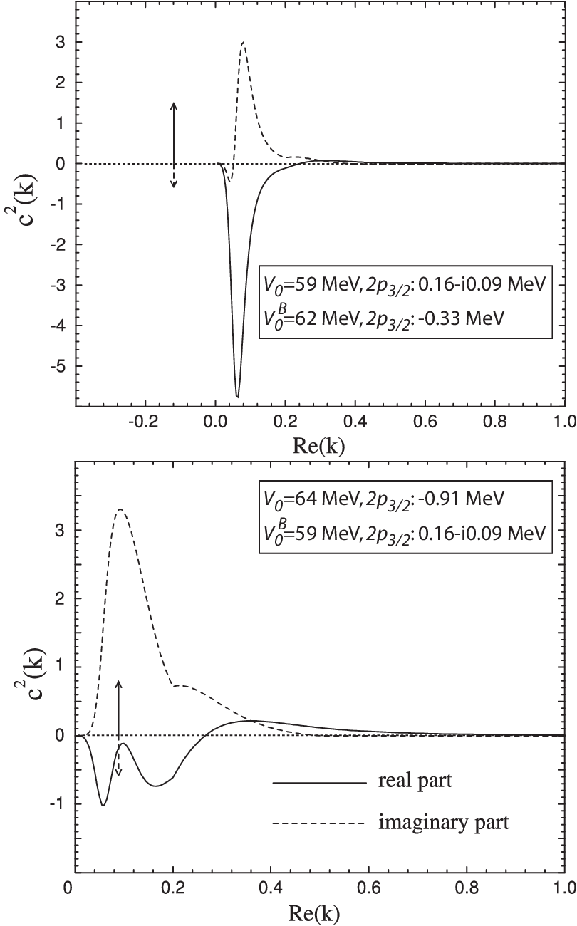
The expansion coefficients (50) are shown in Fig. 5 where the depth of the WS potential is varied to generate a resonant or bound $2p_{3/2}$ state. In both cases, the importance of the scattering continuum is noticeable. This example nicely demonstrates the invalidity of the pole approximation to provide a quantitative description of weakly bound or resonant states.

More examples of s.p. expansions can be found in Refs. [119] (neutrons) and [53] (protons). Let us only mention that in the proton case the role of the scattering continuum is somehow reduced due to the confining effect of the Coulomb barrier, especially at small energies. Still, for a precise description of eigenstates, the scattering component needs to be included.

The discretized basis (42) can be used to extend the completeness relation to the many-body case, in a full analogy with the standard SM in a complete discrete basis, e.g., the HO basis. The many-body basis of GSM corresponds to Slater determinants (SD) built from one-body states constituting the Berggren ensemble:

$$|SD\rangle_{n}=|u_{i_{1}}\cdots u_{i_{A}}\rangle,$$

(51)

where $|u_{i}\rangle$ are properly normalized one-body states (either resonant or scattering) of a generating potential. The completeness of the Berggren ensemble guarantees the closure relation for the many-body GSM basis:

$$\sum_{n}|SD_{n}\rangle\langle SD_{n}|\sim 1,$$

(52)

where $n$ runs over all possible SDs (51). The approximate equality in (52) is a consequence of the continuum discretization.

The GSM Hamiltonian matrix in the basis (52) is complex symmetric. In a standard SM, the Lanczos method is often used to determine the eigenstates of the Hamiltonian matrix. It allows calculating selected states, e.g., ground state and low-lying excited states, in very large configuration spaces. However, the Lanczos method cannot be applied mutatis mutandis to the GSM matrix problem, due to the presence of scattering states. As many-body resonant states are embedded in the discretized continuum of many-body scattering states, the lowest-energy principle cannot be used to guide our choice.

One way of selecting many-body resonant states was proposed in Refs. [117, 143] dealing with systems having two valence nucleons. Here, the selection of two-particle resonances is done with a suitable choice of the contour $L^{+}$. It was realized that by choosing a square-shaped contour, the resonant states appear in the so-called allowed region of the complex-energy plane [117] and this facilitates their identification.

In Fig. 6 the allowed region is a square-shaped area defined by a s.p. contour. Due to the low density of two-particle scattering states in this region, the trajectories of two-particle resonances can be easily followed as the strength of the residual interaction increases.

It has been observed that the two-body resonant states are mostly based on the pole-pole (p-p) configuration, although the role of discretized continuum states (p-c, c-c) in Fig. 6 is not negligible. The result that the correlated two-particle resonant states are built mainly from configurations formed from s.p. resonant states gives strong support for the use of the overlap method discussed below. Unfortunately this convenient method might not be generalized easily to the case of more than two valence particles.

Another solution to the problem of resonant-state selection, particularly useful in the case of several valence nucleons, has been proposed in Ref. [119]. It is based on the overlap method, utilizing the property that the main components of many-body resonant states are built from resonant SD. In the first step, the GSM Hamiltonian is diagonalized in a smaller basis consisting of s.p. resonant states only (a pole approximation). Here, some variant of the Lanczos method can be applied. The diagonalization yields the first-order approximation to many-body resonances $|\Psi_{0}\rangle$. In the second step, $|\Psi_{0}\rangle$ is used as a Lanczos pivot. Diagonalization of the GSM Hamiltonian in this subspace yields many-body eigenstates. The resonant state is the eigenstate $|\Psi\rangle$ which maximizes the overlap $|\langle\Psi_{0}|\Psi\rangle|$. This method identifies the many-body resonant state provided its coupling to the non-resonant continuum is weak, i.e. 10-30%. This condition is usually satisfied, especially if the one-body basis has been optimized by way of the GHF procedure.

Fig. 7 illustrates the overlap technique for $J^{\pi}=0^{+}$ states in ²⁰O considered as a four-neutron system outside the ¹⁶O core [119]. Diagonalization of the GSM Hamiltonian matrix provides complex-energy eigenstates. Compared with Fig. 6, the number of many-body states is much larger and the regular pattern of non-resonant states reflecting the structure of the scattering contour is gone (the figure represents the projection of four-dimensional trajectories onto two dimensional space). While the two lowest (bound) states can be simply identified by inspection, for the higher-lying states it is practically impossible to separate the resonances from the non-resonant continuum. However, the procedure outlined above makes it possible to identify unambiguously the many-body resonance states. It is seen that the resonant states shown in Fig. 7 they all have negligible or very small positive widths, as expected. The many-body resonant states appear to be stable with respect to small changes of the contour (as the physical solutions should not be dependent on the deformation of the basis). On the other hand, the states representing the non-resonant many-body continuum move in the complex energy plane with the contour’s deformation.

Hamiltonian matrix elements between resonant states can be calculated with complex scaling (see Sec. 3). However, this is not the case with scattering states, for which complex-scaled integrals may not converge regardless of the angle of rotation, as is the case for the normalization of scattering states (see Sec. 4.2). In the latter situation, since the result is analytical (Dirac delta), the problem can be dealt with by means of the contour discretization (see Sec. 4.3). However, it is very difficult to calculate matrix elements of general interactions; hence, in the first applications, only localized Hamiltonians were used. Examples are the Gaussian separable interaction [117, 139], the Surface Delta interaction [118, 119], and the Surface Gaussian interaction (SGI) [53] (see Sec. 6.1). For these schematic forces, the calculation of two-body matrix elements is straightforward. In order to deal with realistic interactions, which are very complicated to express and infinite-ranged in shell-model coordinates, a new approach, based on a HO basis expansion technique, had to be devised (see Sec. 6.2).

In the GSM, the electromagnetic (EM) transition selection rules and the angular momentum and isospin algebra do not change compared to the standard SM. However, to calculate the EM transitions, one can no longer use the long wavelength approximation because of the presence of the non resonant continuum. Indeed, for the diagonal EM matrix elements $\langle n_{i}\ell_{i}j_{i}k_{i}|O|n_{f}\ell_{f}j_{f}k_{f}\rangle$ ($k_{i}$ = $k_{f}$) between the scattering states, the complex scaling cannot be carried out. Furthermore, one cannot employ the long wavelength approximation to the EM operators as they behave like $r^{\lambda}$. Without the long wavelength approximation, however, the continuum-continuum matrix elements become finite, because it is always possible to carry out a complex scaling with the Bessel function of the photon $j_{L}(qr)$, as $q\neq 0$. As all the other matrix elements can be regularized, the EM matrix elements are all well defined.

The application of the Berggren ensemble to GSM is associated with the explosive growth in the number of configurations with the number of active particles and the size of the s.p. space. To ensure completeness of the Berggren basis, for each resonant s.p. state $(\ell,j)$, one should include a large number of s.p. scattering states $\{(\ell,j)^{(f)};f=1,\dots,M\}_{\rm c}$ lying on a discretized contour $L_{+}^{\ell_{j}}$. All these states become new active shells; hence, the configuration space of GSM grows extremely fast with the number of contour discretization points. Moreover, the resulting complex-symmetric GSM Hamiltonian matrix is significantly denser than the Hamiltonian matrix of a conventional SM. Hence, taming the dimensionality growth in solving the many-body Schrödinger equation is crucial.

There are several specific features of the dimensional catastrophe in GSM that may facilitate this task. Firstly, of all GSM eigenstates, of major interest are the many-body resonant states. As discussed in Sec. 5.2, these eigenstates represent a narrow class of spatially localized states, immersed in a sea of non-resonant scattering states. Eigenstates of the GSM Hamiltonian in the pole space can serve as the reference vectors, helping to identify resonant eigenstates out of a huge space of all GSM eigenvectors. Hence, instead of a direct diagonalization of the GSM Hamiltonian matrix, a strategy should be developed for an optimization of the scattering space.

The Density Matrix Renormalization Group (DMRG) method was introduced in Ref. [144] to overcome the limitations of Wilson-type renormalization groups to describe strongly correlated 1D lattice systems with short-range interactions (see also recent reviews [145, 146]). Up to now, most of the DMRG studies were focused on equilibrium properties in strongly correlated closed quantum systems (CQS) with a Hermitian density matrix. Nevertheless, non-equilibrium systems involving non-Hermitian and non-symmetric density matrices can also be treated in the DMRG [147]. The DMRG approach is ideally suited to optimize the size of the scattering space in the GSM problem as the properties of the non-resonant shells vary smoothly along the scattering contour. The main idea of the GSM+DMRG truncation algorithm [148, 149] is to gradually consider different s.p. shells of the discretized non-resonant continuum in the configuration space and retain only $N_{\rm opt}$ optimal states dictated by the eigenvalues of the density matrix with the largest modulus. Since the GSM Hamiltonian is complex symmetric, it is the complex (or generalized) variational principle [150, 151, 152] than the usual variational principle that governs the GSM+DMRG algorithm [149].

The iterative GSM+DMRG procedure of constructing the eigenvectors is divided into two phases: the warm-up phase and the sweeping phase. There are two essential conditions which guarantee that the GSM+DMRG method yields correct results. The first one is to ensure that all possible couplings in the many-body wave function, allowed by the symmetries of the problem, are present in the warm-up phase. This means that one should keep all the essential partial waves which are present in DMRG wave functions, even though they may be absent at the pole approximation level. The second condition is to ensure that the reference state $|\Psi_{J}\rangle^{(0)}$, which is a key ingredient in selecting the target state $|\Psi_{J}\rangle$ from the set of all GSM solutions of a given angular momentum and parity at each iteration step, is correctly described.

The DMRG configuration space can be initially divided into two subspaces: $A$ (the reference subspace built from all s.p. resonant shells $\{(n_{1},\ell_{1},j_{1})$, $(n_{2},\ell_{2},j_{2}),\dots\}$ and one representative non-resonant shell for each remaining partial wave $\{(\ell_{p},j_{p}),(\ell_{r},j_{r}),\dots\}$ in the valence space) that is essential to produce many-body couplings, and $B$ (the complementary subspace built from the s.p. non-resonant shells $\{(\ell_{1},j_{1})\}_{\rm c}$, $\{(\ell_{2},j_{2})\}_{\rm c},\dots$). One begins in the warm-up phase by constructing all product states $|k\rangle_{A}$ forming the reference subspace $A$.

The many-body configurations in $A$ can be classified in different families $\{n;j_{A}\}$ according to their number of nucleons $n$ and total angular momentum $j_{A}$. All possible matrix elements of sub-operators of the two-body Hamiltonian acting in $A$ are calculated and stored. The Hamiltonian is then diagonalized in $A$ to provide the zeroth-order approximation to the targeted eigenstate $|J^{\pi}\rangle$, called the reference state $|\Psi_{J}\rangle^{(0)}$. In the next step, the subspace of the first scattering shell $(\ell,j)_{1}$ belonging to the discretized contour $L^{+}$ is added. Within this shell, one constructs all possible many-body states, denoted as $|i\rangle_{B}$ and grouped in $\{n_{B};j_{B}\}$ families, and all matrix elements of sub-operators of the Hamiltonian. This ensemble serves as a basis in which the GSM Hamiltonian is diagonalized. The target state $|\Psi_{J}\rangle$ is selected among the eigenstates of the Hamiltonian as the one having the largest overlap with the reference vector $|\Psi_{J}\rangle^{(0)}$. Based on the expansion:

$$|\Psi_{J}\rangle=\sum_{k_{A},i_{B}}c^{k_{A}(j_{A})}_{i_{B}(j_{B})}\{|k_{A}(j_{A})\rangle\otimes|i_{B}(j_{B})\rangle\}^{J}~~,$$

(53)

by summing over the reference subspace $A$ for a fixed value of $j_{B}$, one obtains the reduced density matrix [153]:

$\displaystyle\rho^{B}_{i_{B}i^{\prime}_{B}}(n_{B},j_{B})\equiv\sum_{k_{A}}c^{k_{A}(j_{A})}_{i_{B}(j_{B})}c^{k_{A}(j_{A})}_{i^{\prime}_{B}(j_{B})}$

(54)

which is complex-symmetric in the metric defining the Berggren ensemble. In the warm-up phase, the reference subspace becomes the ‘medium’ for the ‘system’ part in the $B$ subspace.

Truncation in the system part is dictated by the density matrix. The reduced density matrix is diagonalized and one retains at most ${N}_{\rm opt}$ eigenstates of $\hat{\rho}^{B}$:

$$\hat{\rho}^{B}(n_{B},j_{B})|\alpha\rangle_{B}=w_{\alpha}|\alpha\rangle_{B}$$

(55)

having the largest nonzero values of $|w_{\alpha}|$. Then, one expresses the eigenstates $|\alpha\rangle_{B}$ in terms of the vectors $|i\rangle_{B}$ in $B$:

$$|\alpha\rangle_{B}=\sum_{i}d^{\alpha}_{i}|i\rangle_{B}$$

(56)

and all matrix elements of the sub-operators in these optimized states,

${}_{B}\langle\alpha|O|\beta\rangle_{B}=\sum_{i,i^{\prime}}d^{\alpha}_{i}d^{\beta}_{i^{\prime}}~{}_{B}\langle i|O|i^{\prime}\rangle_{B}$

(57)

are recalculated and stored. In a similar way, the warm-up procedure continues by adding to the system part the configurations containing particles in the next scattering shells until the last shell in $B$ is reached. At this point, all s.p. states have been considered, the warm-up phase ends, and the sweeping phase begins (cf. Refs.  [148, 149] for details). The sequence of sweep-up and sweep-down phases continues until convergence for target eigenvalues is achieved.

References

- [1] J. Dobaczewski, N. Michel, W. Nazarewicz, M. Płoszajczak, and J. Rotureau, Prog. Part. Nucl. Phys. 59 (2007) 432
- [2] J. Okołowicz, M. Płoszajczak, and I. Rotter, Phys. Rep. 374 (2003) 271
- [3] A.M. Lane, and R.G. Thomas, Rev. Mod. Phys 30 (1958) 257
- [4] A.M. Lane, Nucl. Phys. A 35, 676 (1962).
- [5] I.M. Gel’fand and N.Ya. Vilenkin, Generalized Functions, Vol. 4, Academic Press, New York (1961)
- [6] K. Maurin, Generalized Eigenfunction Expansions and Unitary Representations of Topological Groups, Polish Scientific Publishers, Warsaw (1968)
- [7] A. Bohm, The Rigged Hilbert Space and Quantum Mechanics, Lecture Notes in Physics 78, Springer, New York (1978)
- [8] R. de la Madrid, Eur. J. Phys. 26 (2005) 287
- [9] G. Ludwig, Foundations of Quantum Mechanics, Vol. I and II, Springer-Verlag, New York (1983)
- [10] G. Ludwig, An Axiomatic Basis of Quantum Mechanics, Vol. I and II, Springer-Verlag, New York (1983)
- [11] A.F.J. Siegert, Phys. Rev. 56 (1939) 750
- [12] R.E. Peierls, Proc. R. Soc. (London) A 253 (1959) 16
- [13] J. Humblet and L. Rosenfeld, Nucl. Phys. 26 (1961) 529
- [14] P. Lind, Phys. Rev. C 47 (1993) 1903
- [15] C.G. Bollini, O. Civitarese, A.L. De Paoli, and M.C. Rocca, Phys. Lett. B 382 (1996) 205
- [16] L.S. Ferreira, E. Manglione, and R.J. Liotta, Phys. Rev. Lett. 78 (1997) 1640
- [17] R. de la Madrid and M. Gadella, Am. J. Phys. 70 (2002) 626
- [18] E. Kapuścik and P. Szczeszek, Czech. J. Phys. 53 (2003) 1053
- [19] E. Hernandez, A. Járegui, and A. Mondragon, Phys. Rev. A 67 (2003) 022721
- [20] E. Kapuścik and P. Szczeszek, Found. Phys. Lett. 18 (2005) 573
- [21] J. Julve, and F.J. de Urries, quant-ph/0701213.
- [22] R. de la Madrid, AIP Conf. Proc. 885 (2007) 3
- [23]
H.W. Barz, I. Rotter and J. Höhn, Nucl. Phys. A 275 (1977) 111;
I. Rotter, H.W. Barz, and J. Höhn, Nucl. Phys. A 297 (1978) 237;
I. Rotter, Rep. Prog. Phys. 54 (1991) 635. - [24]
R.J. Philpott, Nucl. Phys. A 289 (1977) 109;
D. Halderson and R.J. Philpott, Nucl. Phys. A 321 (1979) 295; ibid. A 359 (1981) 365. - [25]
K. Bennaceur, F. Nowacki, J. Okołowicz and M. Płoszajczak, J. Phys. G 24 (1998) 1631 ;
Nucl. Phys. A 651 (1999) 289 ; Nucl. Phys. A 671 (2000) 203 ;
R. Shyam, K. Bennaceur, J. Okołowicz and M. Płoszajczak, Nucl. Phys. A 669 (2000) 65 ;
K. Bennaceur, N. Michel, F. Nowacki, J. Okołowicz and M. Płoszajczak, Phys. Lett. B 488 (2000) 75;
N. Michel, J. Okołowicz, F. Nowacki and M. Płoszajczak, Nucl. Phys. A 703 (2002) 202. - [26] J. Rotureau, J. Okołowicz, and M. Płoszajczak, Phys. Rev. Lett. 95 (2005) 042503 ; Nucl. Phys. A 767 (2006) 13
- [27] A. Volya and V. Zelevinsky, Phys. Rev. Lett. 94, (2005) 052501 ; Phys. Rev. C 74, (2006) 064314
- [28] B. Blank and M. Płoszajczak, Rep. Prog. Phys. 71 (2008) 046301.
- [29] G. Gamow, Z. Phys. 51 (1928) 204
- [30] R.W. Gurney and E.U. Condon, Phys. Rev. 33 (1929) 127
- [31] A.I. Baz, Ya.B. Zel’dovich, and A.M. Perelomov, Scattering Reactions and Decay in Nonrelativistic Quantum Mechanics, Israel Program for Scientific Translations, Jerusalem (1969)
- [32] T. Berggren, Nucl. Phys. A 109 (1968) 265
- [33] Ya.B. Zel’dovich, Zh. Eksp. i Theor. Fiz. 39 (1960) 776
- [34] N. Hokkyo, Prog. Theor. Phys. 33 (1965) 1116
- [35] W.J. Romo, Nucl. Phys. A 116 (1968) 617
- [36] J. Zimányi, M. Zimányi, B. Gyarmati, and T. Vertse, Acta Phys. Hung. 28 (1970) 251
- [37] B. Gyarmati, T. Vertse, J. Zimányi, and M. Zimányi, Phys. Rev. C 1 (1970) 1
- [38] J. Bang and J. Zimányi, Nucl. Phys. A 139 (1969) 534
- [39] B. Gyarmati and T. Vertse, Nucl. Phys. A 160 (1971) 523
- [40] R. Newton, Scattering Theory of Waves and Particles, Springer-Verlag, New York, Heidelberg (1982)
- [41] H.M. Nussenzveig, Causality and Dispersion Relations, Academic Press, New York (1972)
- [42] J.R. Taylor, Scattering Theory, Wiley, New York (1972)
- [43] W. Domcke, J. Phys. B 14 (1981) 4889
- [44] V.I. Kukulin, Theory of Resonances, Kluver Academic Publishers, Dordrecht, Boston, London (1989)
- [45] A.B. Migdal, A.M. Perelomov, and V.S. Popov, Sov. J. Nucl. Phys. 14 (1972) 488
- [46] H.M. Nussenzveig, Nucl. Phys. 11 (1959) 499
- [47] R. Zavin and N. Moiseyev, J. Phys. A 37 (2004) 4619
- [48] T. Vertse, P. Curutchet, R.J. Liotta, and J. Bang, Acta Phys. Hung. 65 (1989) 305
- [49] R. Id Betan, R.J. Liotta, N. Sandulescu, and T. Vertse, Phys. Lett. B 584 (2004) 48
- [50] R. Id Betan, R.J. Liotta, N. Sandulescu, and T. Vertse, Phys. Rev. C 72 (2005) 054322
- [51] N. Michel, W. Nazarewicz, M. Płoszajczak, and J. Rotureau, Phys. Rev. C 74 (2006) 054305
- [52] N. Dunford and J.T. Schwartz, Linear Operators, Wiley Classics Library (1988)
- [53] N. Michel, W. Nazarewicz, and M. Płoszajczak, Phys. Rev. C 70 (2004) 064313
- [54] N. Michel, J. Math. Phys. 49 (2008) 022109
- [55] A. Mukhamedzhanov and M. Akin, arXiv:nucl-th/0602006
- [56] N. Mukunda, Am. J. Phys. 49 (1978) 910
- [57] W.D. Heiss, J. Phys. A 37 (2004) 2455
- [58] P.A.M. Dirac, The Principles of Quantum Mechanics, Clarendon, Oxford (1958)
- [59] A. Bohm, M. Gadella, and S. Maxon, Computers Math. Applic. 34 (1997) 427
- [60] O. Civitarese and M. Gadella, Phys. Reports 396 (2004) 41
- [61] G. Garcia-Calderon and R. Peierls, Nucl. Phys. A 265 (1976) 443
- [62] Y.B. Zel’dowich, JETP (Sov. Phys.) 22 (1961) 542
- [63] E. Hernandez, and A. Mondragon, Phys. Rev. C 29 (1984) 722
- [64] E. Hernández, A. Mondragón, and J. M. Velásquez-Arcos, Ann. der Physik (Leipzig) 48 (1991) 503
- [65] M.J. Corinthios, IEE Proc.-Vis. Image Signal Process., 150 (2003) 69 ; 152 (2005) 97
- [66] K. Sasada, Spectral Analysis of the Conductance of Open Quantum Dots, PhD-thesis, University of Tokyo (2007).
- [67] W.J. Romo, Nucl. Phys. A 419 (1984) 333
- [68] T. Berggren, Phys. Lett. B 73 (1978) 389
- [69] T. Berggren, Phys. Lett. B 373 (1996) 1
- [70] A. Bohm, and M. Gadella, Lecture Notes in Physics, Vol. 348, Springer-Verlag, Berlin; A. Bohm, Int. J. Theor. Phys. 42 (2003) 2317
- [71] O. Civitarese, M. Gadella, and R. Id Betan, Nucl. Phys. A 660 (1999) 255
- [72] A. Bürgers and J-M. Rost, J. Phys. B 29 (1996) 3825
- [73] H. Friedrich, Theoretical Atomic Physics, Chapter 1, Springer-Verlag, New York (1991)
- [74] J. Bang, F.A. Gareev, M.H. Gizzatkulov, and S.A. Goncharov, Nucl. Phys. A 309 (1978) 381
- [75] G. Garcia-Calderon, Nucl. Phys. A 448 (1986) 560
- [76] T. Vertse, P. Curutchet, R.J. Liotta, J. Bang, and N. Van Giai, Phys. Lett. B 264 (1991) 1
- [77] T. Berggren and P. Lind, Phys. Rev. C 47 (1993) 768
- [78] T. Alferova and N. Elander, Int. J. Quantum Chem. 97 (2004) 922
- [79] M. Rittby, N. Elander, and E. Brändas, Lecture Notes in Physics 325 (1989) 129
- [80] P. Krylstedt, C. Carlsund, and N. Elander, J Phys. B 22 (1989) 1051
- [81] B. Milek and R. Reif, Nucl. Phys. A 458 (1986) 354
- [82] B. Gyarmati, A.T. Kruppa, and J. Révai, Nucl. Phys. A 326 (1979) 119
- [83] F.A. Gareev, M.Ch. Gizzatkulov, and J. Révai, Nucl. Phys. A 286 (1978) 512
- [84] T. Vertse, P. Curutchet, O. Civitarese, L.S. Ferreira, and R.J. Liotta, Phys. Rev. C 37 (1988) 876
- [85] P. Curutchet, T. Vertse, and R.J. Liotta, Phys. Rev. C 39 (1989) 1020
- [86] T. Vertse, P. Curutchet, and R.J. Liotta, Lecture Notes in Physics 325 (1989) 179
- [87] G.G. Dussel, R.J. Liotta, H. Sofia, and T. Vertse, Phys. Rev. C 46 (1992) 558
- [88] P. Lind, R.J. Liotta, E. Maglione, and T. Vertse, Z. Phys. A 347 (1994) 231
- [89] O.I. Tolstikhin, V.N. Ostrovsky, and H. Nakamura, Phys. Rev. A 58 (1998) 2077
- [90] K. Toyota, T. Morishita, and S. Watanable, Phys. Rev. C 72 (2005) 062718
- [91] K. Toyota, T. Morishita, and S. Watanable, Phys. Rev. C 63 (2001) 052721
- [92] T. Myo, A. Ohnishi, and K. Katō, Prog. Theor. Phys. 99 (1998) 801
- [93] G. Hagen and J.S. Vaagen, Phys. Rev. C 73 (2006) 034321
- [94] T. Vertse, K.F. Pál, and Z. Balogh, Comput. Phys. Comm. 27 (1982) 309
- [95] L.Gr. Ixaru, Numerical Methods for Differential Equations, Reidel, Dordrecht (1984)
- [96] L.Gr. Ixaru, M. Rizea, and T. Vertse, Comput. Phys. Comm. 85 (1995) 217
- [97] T. Zhanlav and I.V. Puzynin, Sov. J. Nucl. Phys. 55 (1992) 349
- [98] A.T. Kruppa and Z. Papp, Comput. Phys. Comm. 36 (1985) 59
- [99] T. Vertse, R.J. Liotta, and E. Maglione, Nucl. Phys. A 584 (1995) 13
- [100] J. Blomqvist, O. Civitarese, E.D. Kirchuk, R. J. Liotta, and T. Vertse, Phys. Rev. C 53 (1996) 2001
- [101] R.J. Liotta, E. Maglione, N. Sandulescu, and T. Vertse, Phys. Lett. B 367 (1996) 1
- [102] N. Sandulescu, O. Civitarese, R.J. Liotta, and T. Vertse, Phys. Rev. C 55 (1997) 1250
- [103] T. Vertse, A. T. Kruppa, R. J. Liotta, W. Nazarewicz, N. Sandulescu, and T. R. Werner, Phys. Rev. C 57 (1998) 3089
- [104] T. Vertse, A.T. Kruppa, and W. Nazarewicz, Phys. Rev. C 61 (2000) 064317
- [105] G.G. Dussel, R. Id Betan, R.J. Liotta, and T. Vertse, Nucl. Phys. A 789 (2007) 182
- [106] J. Dobaczewski, W. Nazarewicz, T.R. Werner, J.-F. Berger, C.R. Chinn, and J. Dechargé, Phys. Rev. C 53 (1996) 2809
- [107] D.S. Delion and J. Suhonen, Phys. Rev. C 61 (2000) 024304
- [108] A. Bianchini, R.J. Liotta, and N. Sandulescu, Phys. Rev. C 63 (2001) 024610
- [109] E. Maglione, L.S. Ferreira, and R.J. Liotta, Phys. Rev. Lett. 81 (1998) 538
- [110] E. Maglione, L.S. Ferreira, and R.J. Liotta, Phys. Rev. C 59 (1999) R589
- [111] K. Rykaczewski, et al., Phys. Rev. C 60 (1999) 011301
- [112] A.T. Kruppa, B. Barmore, W. Nazarewicz, and T. Vertse, Phys. Rev. Lett. 84 (2000) 4549
- [113] B. Barmore, A.T. Kruppa, W. Nazarewicz, and T. Vertse, Phys. Rev. C 62 (2000) 054315
- [114] A.T. Kruppa and W. Nazarewicz, Phys. Rev. C 69 (2004) 054311
- [115] I. Martel, M.J.G. Borge, J. Gomez-Camacho, A. Poves, J. Sanchez, and O. Tengblad, Nucl. Phys. A 694 (2001) 424
- [116] S. A. Gurvitz, P.B. Semmes, W. Nazarewicz, and T. Vertse, Phys. Rev. A 69 (2004) 042705
- [117] R. Id Betan, R.J. Liotta, N. Sandulescu, and T. Vertse, Phys. Rev. Lett. 89 (2002) 042501
- [118] N. Michel, W. Nazarewicz, M. Płoszajczak, and K. Bennaceur, Phys. Rev. Lett. 89 (2002) 042502
- [119] N. Michel, W. Nazarewicz, M. Płoszajczak, and J. Okołowicz, Phys. Rev. C 67 (2003) 054311
- [120] R. Id Betan, A.T. Kruppa, and T. Vertse, Phys. Rev. C, in press.
- [121] W.P. Reinhardt, Ann. Rev. Phys. Chem. 33 (1982) 223
- [122] J. Aguilar and J. M. Combes, Commun. Math. Phys. 22 (1971) 269
- [123] E. Balslev and J. M. Combes, Commun. Math. Phys. 22 (1971) 280
- [124] B. Simon, Commun. Math. Phys. 27 (1972) 1
- [125] B. Simon, Phys. Lett. A 71 (1979) 211
- [126] A. Csótó, B. Gyarmati, A.T. Kruppa, K.F. Pál, and N. Moiseyev, Phys. Rev. A 41 (1990) 3469
- [127] R. Lefebvre, Phys. Rev. A 46 (1992) 6071
- [128] A.T. Kruppa, R.G. Lovas, and B. Gyarmati, Phys. Rev. C 37 (1988) 383
- [129] A.T. Kruppa, P-H Heenen, H. Flocard, and R. J. Liotta, Phys. Rev. Lett. 79 (1997) 2217
- [130] A. T. Kruppa, P-H Heenen, and R. J. Liotta, Phys. Rev. C 63 (2001) 044324
- [131] C. A. Nicolaides, H. J. Gotsis, M. Chrysos, and Y. Komninos, Chem. Phys. Letters 168 (1990) 570
- [132] T.N. Rescigno, M. Baertschy, W.A. Isaacs, and C.W. McCurdy, Science 286 (1999) 2474
- [133] J.Zs. Mezei, A.T. Kruppa, and K. Varga, Few-Body Systems 41 (2007) 233
- [134] T. Li and R. Shakeshaft, Phys. Rev. A 71 (2005) 052505
- [135] Y.K. Ho, Phys. Rev. A 19 (1979) 2347
- [136] A.T. Kruppa, R. Suzuki, and K. Katō, Phys. Rev. C 75 (2007) 044602
- [137] D. Vautherin and M. Vénéroni, Phys. Lett. B 25 (1957) 175
- [138] G. Hagen, M. Hjorth-Jensen, and N. Michel, Phys. Rev. C 73 (2006) 064307
- [139] G. Hagen, M. Hjorth-Jensen, and J.S. Vaagen, Phys. Rev. C 71 (2005) 044314
- [140] N. Michel, M. Stoitsov, and K. Matsuyanagi, in preparation
- [141] S.T. Belyaev, A.V. Smirnov, S.V. Tolokonnikov, and S.A. Fayans, Sov. J. Nucl. Phys. 45 (1987) 783
- [142] N. Michel, W. Nazarewicz, and M. Płoszajczak, Proc. New Developments in Nuclear Self-Consistent Mean-Field Theories, YITP, Kyoto, Japan, YITP-W-05-01, B32 (2005)
- [143] R. Id Betan, R.J. Liotta, N. Sandulescu, and T. Vertse, Phys. Rev. C 67 (2003) 014322
- [144] S.R. White, Phys. Rev. Lett. 69 (1992) 2363; Phys. Rev. B 48 (1993) 10345
- [145] J. Dukelsky and S. Pittel, Rep. Prog. Phys. 67 (2004) 513
- [146] U. Schollwöck, Rev. Mod. Phys. 77 (2005) 259
- [147] E. Carlon, M. Henkel, and U. Schollwöck, Eur. J. Phys. B 12 (1999) 99
- [148] J. Rotureau, N. Michel, W. Nazarewicz, M. Płoszajczak, and J. Dukelsky, Phys. Rev. Lett. 97 (2006) 110603
- [149] J. Rotureau, N. Michel, W. Nazarewicz, M. Płoszajczak, and J. Dukelsky, in preparation
- [150] N. Moiseyev, P.R. Certain, and F. Weinhold, Mol. Phys. 36, 1613 (1978).
- [151] N. Moiseyev, Phys. Rep. 302, 212 (1998).
- [152] N. Moiseyev, Chem. Phys. Lett. 99, 364 (1983).
- [153] I. McCulloch and M. Gulacsi, Europhys. Lett. 57 (2002) 852
- [154] M. Hjorth-Jensen, T.T.S. Kuo, and E. Osnes, Phys. Rep. 261 (1995) 125
- [155] K. Suzuki and S.Y. Lee, Prog. Theor. Phys. 64 (1980) 2091; K. Suzuki, Prog. Theor. Phys. 68 (1982) 246; K. Suzuki, and R. Okamoto, Prog. Theor. Phys. 93 (1995) 905
- [156] S. Bogner, T.T.S. Kuo, and A. Schwenk, Phys. Rep. 386 (2003) 1
- [157] R. Wiringa, V.G.J. Stoks, and R. Schiavilla, Phys. Rev. C 51 (1995) 38
- [158] R. Machleidt, Phys. Rev. C 63 (2001) 024001
- [159] E. Epelbaum, Prog. Part. Nucl. Phys. 57 (2006) 654
- [160] R.D. Lawson, Theory of the Nuclear Shell Model, Clarendon-Press, Oxford (1980)
- [161] R. Balian and E. Brezin, Nuovo Cim. 61 (1969) 403
- [162] C.W. Wong and D.M. Clement, Nucl. Phys. A 183 (1972) 210
- [163] C.L. Kung, T.T.S. Kuo, and K.F. Ratcliff, Phys. Rev. C 19 (1979) 1063
- [164] G. Hagen, D.J. Dean, M. Hjorth-Jensen, and T. Papenbrock, Phys. Lett. B 656 (2007) 169
- [165] H.J. Lipkin, Phys. Rev. 110 (1958) 1395
- [166] R.R. Whitehead, A. Watt, B.J. Cole, and I. Morrison, Adv. Nucl. Phys. 9 (1977) 123
- [167] Y. Suzuki and K. Ikeda, Phys. Rev. C 38 (1988) 410
- [168] K. Katō, private communication
- [169] A. Bohr and B.R. Mottelson, Nuclear Structure, Vol. 1, W.A. Benjamin, New York (1969)
- [170] N.K. Glendenning, Ann. Rev. Nucl. Sci. 13 (1963) 191; N.K. Glendenning, Direct Nuclear Reactions, Academic Press Inc. (1983)
- [171] P. Fröbrich and R. Lipperheide, Theory of Nuclear Reactions, Oxford Science Publications, Clarendon Press, Oxford (1996)
- [172] M.B. Tsang, Jenny Lee, and W.G. Lynch, Phys. Rev. Lett. 95 (2005) 222501
- [173] P.G. Hansen and J.A. Tostevin, Ann. Rev. Nucl. Part. Sci. 53 (2003) 219
- [174] A. Gade et al., Eur. Phys. J. A 25 (2005) s01, 251; D. Bazin et al., Phys. Rev. Lett. 91 (2003) 012501
- [175] E.P. Wigner, Phys. Rev. 73 (1948) 1002
- [176] P.R. Malmberg, Phys. Rev. 101 (1956) 114
- [177] J.T. Wells, A.B. Tucker, and W.E. Meyerhof, Phys. Rev. 131 (1963) 1644
- [178] C.F. Moore et al., Phys. Rev. Lett. 17 (1966) 926
- [179] S. Abramovich, B. Guzhovskij, and L. Lasarev, Sov. J. Part. Nucl. 23 (1992) 129
- [180] G. Breit Phys. Rev. 107 (1957) 1612
- [181] A.M. Lane, Phys. Lett. B 33 (1970) 274
- [182] C. Hategan, Ann. Phys. 116 (1978) 77
- [183] A.I. Baz, JETP (Sov. Phys.) 6 (1957) 709
- [184] R.G. Newton, Phys. Rev. 114 (1959) 1611
- [185] W.E. Meyerhof, Phys. Rev. 129 (1963) 692
- [186] N. Michel, W. Nazarewicz, and M. Płoszajczak, Phys. Rev. C 75 (2007) 031301(R)
- [187] N. Michel, W. Nazarewicz, and M. Płoszajczak, Nucl. Phys. A 794 (2007) 29
- [188] W.H. Dickhoff, and C. Barbieri, Prog. Part. Nucl. Phys. 52 (2004) 377
- [189] L.D. Blokhintsev, I. Borbely, and E.I. Dolinskii, Sov. J. Part. Nucl. 8 (1977) c485
- [190] N.K. Timofeyuk, L.D. Blokhintsev, and J.A. Tostevin, Phys. Rev. C 68 (2003) 021601(R)
- [191] T. Myo, K. Katō, S. Aoyama, and K. Ikeda, Phys. Rev. C 63 (2001) 054313; T. Myo, K. Katō, S. Aoyama, and K. Ikeda, Phys. Lett. B 576 (2003) 281
- [192] T. Myo, K. Katō, and K. Ikeda, Phys. Rev. C 76 (2007) 054309
- [193] K. Ikeda, Nucl. Phys. A 538 (1992) 355c; S. Mukai, S. Aoyama, K. Katō, and K. Ikeda, Prog. Theor. Phys. 99 (1998) 381; Y. Tosaka, Y. Suzuki, and K. Ikeda, Prog. Theor. Phys. 83 (1990) 1140
- [194] H. Masui, K. Katō, and K. Ikeda, Phys. Rev. C 75 (2007) 034316
- [195] K. Ikeda, N. Takigawa, and. H. Horiuchi, Prog. Theor. Phys. Suppl. Extra Number, 464 (1968)
- [196] I. Tanihata et al., arXiv:0802.1778
- [197] M.V. Berry, Proc. R. Soc. London, Ser. A 392 (1984) 45
- [198] H.-M. Lauber, P. Weidenhammer, and D. Dubbers, Phys. Rev. Lett. 72 (1994) 1004; D.E. Manolopoulos and M.S. Child, Phys. Rev. Lett. 82 (1999) 2223; F. Pistolesi and N. Manini. Phys. Rev. Lett. 85 (2000) 1585; C. Dembowski et al., Phys. Rev. Lett. 86 (2001) 787
- [199] T. Kato, Perturbation Theory for Linear Operators, Springer Verlag, Berlin (1995)
- [200] M.R. Zirnbauer, J.J.M. Verbaarschot, and H.A. Weidenmüller, Nucl. Phys. A 411 (1983) 161
- [201] W.D. Heiss and W.-H. Steeb, J. Math. Phys. 32 (1991) 3003