Our building block is an extended $G_{T\times U}\equiv SU(N_{T})\times SU(N_{U})$ technicolor (TC) gauge theory. The matter content constitutes of techniquarks $Q^{a}_{f}$ charged under the representation $R_{T}$ of the TC group $SU(N_{T})$ and Dirac techniunparticle fermions $\Psi^{A}_{s}$ charged under the representation $R_{U}$ of the unparticle group $SU(N_{U})$, where $a/A=1\ldots{\rm dim}{[R_{T/U}]}$ and $f/s=1\ldots F/S$ denote gauge and flavor indices respectively. We will first describe the (walking) TC and (techni)unparticle sectors separately before addressing their common dynamical origin. A graphical illustration of the scenario is depicted in Fig. 1 as a guidance for the reader throughout this section.

In the TC sector the number of techniflavors, the matter representation and the number of colors are arranged in such a way that the dynamics is controlled by a near conformal (NC) IR fixed point⁵⁵ 5 There are a number of ways of achieving (near) conformal dynamics as summarized in [29]. The state-of-the-art phase diagram [26, 27] and new tools [25] to construct viable NC nonsupersymmetric gauge theory are reported in [3].. In this case the gauge coupling reaches almost a fixed point around the scale $\Lambda_{\cal T}\gg M_{W}$, with $M_{W}$ the mass of the electroweak gauge boson. The TC gauge coupling, at most, gently rises from this energy scale down to the electroweak one. The coupling is said to walk ⁶⁶ 6 Such models are known as walking TC [30]. They are preferred over QCD-like TC models by the electroweak precision data. In particular, the S-parameter receives a negative contribution for NC models [31]. A large class of phenomenologically viable models have been identified [32, 27, 29, 3] of which Minimal Walking Technicolor (MWT) and Partially Gauged Technicolor (PGT) constitute two relevant examples.. Around the electroweak scale the TC dynamics triggers the spontaneous breaking of the electroweak symmetry through the formation of the technifermion condensate, which therefore has the quantum numbers of the SM Higgs boson. The associated Goldstone bosons (technipions) then become the longitudinal degrees of freedom of the electroweak bosons in exact formal analogy to the SM. In the simplest TC models the technipion decay constant $F_{T}$ is related to the weak scale as $2M_{W}=gF_{T}$ ($g$ is the weak coupling constant) and therefore $F_{T}\simeq 250$ GeV. The TC scale, analogous to $\Lambda_{\rm QCD}$ for the strong force, is roughly $\Lambda_{TC}\sim 4\pi F_{T}$.

Now we turn our attention to the unparticle sector. Here the total number of massless techniunparticle flavors $S$ is balanced against the total number of colors $N_{U}$ in such a way that the theory, per se, is asymptotically free and admits a nonperturbative IR fixed point. The energy scale around which the IR fixed point starts to set in is indicated with $\Lambda_{\cal U}\gg M_{W}$.

It might be regarded as natural to assume that the unparticle and the TC sectors have a common dynamical origin, e.g. are part of a larger gauge group at energies above $\Lambda_{\cal T}$ and $\Lambda_{\cal U}$. We would like to point out that the relative ordering between $\Lambda_{\cal T}$ and $\Lambda_{\cal U}$ is of no particular relevance for our scenario. The low energy relics of such a unified-type model are four-Fermi operators allowing the two sectors to communicate with each other at low energy. The unparticle sector will then be driven away from the fixed point due to the appearance of the electroweak scale in the TC sector.

The model, of which further details are presented in section 2 resembles models of extended technicolor (ETC) [3], where the techniunparticles play the role of the SM fermions. We refer to these type of models as Extended Techni-Unparticle (ETU) models⁷⁷ 7 The work by Georgi and Kats [33] on a two dimensional example of unparticles triggered this work.. At very high energies $E\gg M_{\cal U}$ the gauge group $G_{T\times U}$ is thought to be embedded in a simple group $G_{\rm TU}\supset G_{T\times U}$. At around the scale ${M_{\cal U}}$ the ETU group is broken to $G_{TU}\to G_{T\times U}$ and the heavy gauge fields receive masses of the order of ${M_{\cal U}}$ and play the role of the messenger sector. Below the scale ${M_{\cal U}}$ the massive gauge fields decouple and four-Fermi operators emerge, which corresponds to the first step of the scenario, e.g. Eq. (1) and Fig. 1. Without committing to the specific ETU dynamics the interactions can be parametrized as:

$\displaystyle{\cal L}_{<{M_{\cal U}}}^{\rm eff}=\alpha\frac{\bar{Q}Q\,{\bar{\Psi}\Psi}}{{M_{\cal U}^{2}}}+\beta\frac{{\bar{Q}Q}{\bar{Q}Q}}{{M_{\cal U}^{2}}}+\gamma\frac{{\bar{\Psi}\Psi}{\bar{\Psi}\Psi}}{{M_{\cal U}^{2}}}\,.$

(4)

The coefficients $\alpha$, $\beta$ and $\gamma$ (the latter should not be confused with an anomalous dimension) are of order one, which can be calculated if the gauge coupling $g_{\rm TU}$ is perturbative. The Lagrangian (4) is the relic of the ETU(ETC) interaction and gives rise to two sources of dynamical chiral symmetry breaking in addition to the intrinsic dynamics of the groups $G_{T/U}$. These are contact interactions of the type emphasized in [34]. Firstly, when one fermion pair acquires a VEV then the $\alpha$-term turns into a tadpole and induces a VEV for the other fermion pair. This is what happens to the unparticle sector when the TC sector, or the SM Higgs [10], breaks the electroweak symmetry. Secondly, the $\gamma$ term corresponds to a Nambu$-$Jona-Lasino type interaction which may lead to the formation of a VEV, for sufficiently large $\gamma$. This mechanism leads to breaking of scale invariance even in the absence of any other low energy scale. Let us parenthetically note that this mechanism is operative in models of top condensation, c.f. the TC report [35] for an overview. However, based on our analysis in the appendix A we shall neglect this mechanism in the sequel of this paper. We shall refer to these two mechanism as $\alpha/\gamma$-induced condensates.

At the scale $\Lambda_{\cal U}\gg M_{W}$ the unparticle gauge sector flows into an IR fixed point and the UV operator ${\cal O}_{\rm UV}=\bar{\Psi}\Psi$ becomes the composite unparticle operator ${\cal O}_{\rm IR}\equiv{\cal O}_{\cal U}$ with scaling dimension ${d_{\cal U}}\equiv 3-\gamma_{\cal U}$ ⁸⁸ 8 The parametrization ${d_{\cal U}}\equiv 3-\gamma_{\cal U}$ will be standard throughout the entire paper and in the text the scaling dimension ${d_{\cal U}}$ and the anomalous dimension $\gamma_{\cal U}$ will be used interchangeably.,

$$(\bar{\Psi}\Psi)_{UV}\sim\Lambda_{\cal U}^{\gamma_{\cal U}}{\cal O}_{{\cal U}}\;;\qquad M_{W}\ll\Lambda_{{\cal U}}\ll{M_{\cal U}}\ .$$

(5)

Note, the anomalous dimension $\gamma_{\cal U}$ of the operator has to satisfy $\gamma_{\cal U}\leq 2$ due to unitarity bounds of the representations of the conformal group [36]. The Lagrangian then simply becomes

$\displaystyle{\cal L}^{\rm eff}_{\Lambda_{\cal U}}=\alpha^{\prime}\,\frac{\bar{Q}Q\,\Lambda_{\cal U}^{\gamma_{\cal U}}{\cal O}_{\cal U}}{{M_{\cal U}^{2}}}+\beta^{\prime}\,\frac{\bar{Q}Q\bar{Q}Q}{{M_{\cal U}^{2}}}+\gamma^{\prime}\,\frac{\Lambda_{\cal U}^{2\gamma_{\cal U}}\,{\cal O}_{\cal U}{\cal O}_{\cal U}}{{M_{\cal U}^{2}}}\,.$

(6)

This realizes the second step in the scenario, c.f. Fig. 1 and Eq. (1). The matching coefficients $\alpha^{\prime},\beta^{\prime},\gamma^{\prime}$ (6) are related to $\alpha,\beta,\gamma$ (4) by order one coefficients. The $\alpha$-term in Eq. (6) is similar to the unparticle-Higgs interaction in Eq. (3).

The composite operator $\bar{Q}Q$ can be treated in analogy to $\bar{\Psi}\Psi$ in (5),

$$(\bar{Q}Q)_{UV}\sim\Lambda_{\cal T}^{\gamma_{\cal T}}{\cal O}_{\cal T}\;;\qquad\Lambda_{TC}\ll\Lambda_{\cal T}\ll M_{\cal U}\,,$$

(7)

up to logarithmic corrections which are negligible. Contrary to the unparticle sector the TC gauge dynamics break scale invariance through the formation of an intrinsic condensate

$$\langle{\cal O}_{\cal T}\rangle_{\Lambda_{\cal T}}\simeq{w_{T}^{\gamma_{\cal T}}}\Lambda_{TC}^{d_{\cal T}}\equiv{w_{T}^{\gamma_{\cal T}}}\Lambda_{TC}^{3-\gamma_{\cal T}}\,,\quad{w_{T}}\equiv\Big(\frac{\Lambda_{\cal T}}{\Lambda_{TC}}\Big)\ .$$

(8)

The estimate of the VEV is based on scaling from QCD and renormalization group evolution.

The relevant terms contained in the low energy effective theory around the electroweak scale are⁹⁹ 9 Note that in QCD-like TC models (the gauge coupling displays a running behavior rather than a walking one) one would set $\gamma_{\cal T}\simeq 0$ in Eqs. (8) and (9).:

$${\cal L}_{\Lambda_{\cal T}}^{\rm eff}=\alpha^{\prime}\,{w_{T}^{\gamma_{\cal T}}}\,\frac{\Lambda_{TC}^{3}\,\Lambda_{\cal U}^{\gamma_{\cal U}}{\cal O}_{\cal U}}{{M_{\cal U}^{2}}}+\gamma^{\prime}\,\frac{\Lambda_{\cal U}^{2\gamma_{\cal U}}{\cal O}_{\cal U}{\cal O}_{\cal U}}{{M_{\cal U}^{2}}}+..$$

(9)

This step involves another matching procedure but we shall not introduce further notation here and denote the matching coefficients by simple primes only. As stated previously the TC condensate drives the TC gauge sector away from the fixed point and the coupling increases towards the IR. The sector is then replaced by a low energy effective chiral Lagrangian featuring the relevant composite degrees of freedom [37, 35]. The lightest isosinglet composite scalar, with $J^{PC}=0^{++}$ quantum numbers, is the composite Higgs. For further details c.f. appendix F of reference [3] as well as [38]. The linear realization of the chiral Lagrangian of the TC model will be discussed in section 2.

We shall now investigate how the $\alpha$-term in (9) induces a VEV for the unparticle. In a theory with canonically normalized fields the mass term, if present, has to be included for the minimization of the potential. In the unparticle setup we do not have explicit mass terms but there is a continuous mass spectrum and it is not immediately clear how to proceed. Yet we can make use of the deconstructed version of unparticles, proposed by Stephanov [39], in order to imitate the situation of isolated masses [10]. The continuous spectrum is deconstructed into an infinite tower of massive particles,

$${\cal O}_{\cal U}(x)=\sum_{n}f_{n}\varphi_{n}(x)\,;\qquad\left\{\begin{array}[]{l}f_{n}^{2}=\Delta^{2}\,\frac{B_{d_{\cal U}}}{2\pi}(M_{n}^{2})^{{d_{\cal U}}-2}\\[2.84544pt] M_{n}^{2}=n\Delta^{2}\\ \end{array}\right.\,,$$

(10)

with an adjusted residuum $f_{n}$ and a finite spacing $\Delta$ in units of the mass. The spectral function $\rho_{d_{\cal U}}$ of the operator above is given by

$$\rho_{d_{\cal U}}(P^{2})\theta(P_{0})=\sum_{n}\delta(P^{2}-P_{n}^{2})|\langle 0|{\cal O}_{\cal U}|P_{n}\rangle|^{2}\quad\rightarrow\quad\rho_{d_{\cal U}}(s)\equiv\frac{B_{d_{\cal U}}}{2\pi}s^{{d_{\cal U}}-2}\theta(s)\,.$$

(11)

The square root of $B_{d_{\cal U}}$ defines the strength with which a state couples to the unparticle operator. The sum above is a mnemonic for the sum over all the possible states in the Hilbert space. The propagator then follows from the spectral function from the Källén-Lehmann representation (A.11). The factor $B_{d_{\cal U}}$ corresponds to $A_{d_{\cal U}}$ in [4], but we have chosen to denote it by a different letter since, as we shall see, our model demands a different form. The value ${d_{\cal U}}=2$ in (11) is the dividing value between the IR and UV sensitive domains and will play a crucial role later on. Other regularizations than the one in Eq. (10) are possible [39]. Therefore, no physical interpretation should be attached to it. The Lagrangian (9) with added mass terms becomes

$${\cal L}=\bar{\alpha}\sum_{n}f_{n}\varphi_{n}+\bar{\gamma}\sum_{n,m}f_{n}f_{m}\varphi_{n}\varphi_{m}-\frac{1}{2}\sum_{n}M_{n}^{2}\varphi_{n}^{2}\,,$$

(12)

with

$$\bar{\alpha}\equiv\alpha^{\prime}w_{T}^{\gamma_{\cal T}}\frac{\Lambda_{TC}^{3}\Lambda_{\cal U}^{\gamma_{\cal U}}}{{M_{\cal U}^{2}}}\,,\qquad\bar{\gamma}\equiv\gamma^{\prime}\frac{\Lambda_{\cal U}^{2\gamma_{\cal U}}}{{M_{\cal U}^{2}}}\,,$$

(13)

being the prefactors of ${\cal O}_{\cal U}$ and ${\cal O}_{\cal U}^{2}$ in (9), with mass dimensions $[\bar{\alpha}]=\gamma_{\cal U}+1$ and $[\bar{\gamma}]=2\gamma_{\cal U}-2$. The equation of motion (e.o.m.) for the operator $\varphi_{n}$ is

$$\bar{\alpha}f_{n}+2\bar{\gamma}f_{n}(\sum_{m}f_{m}\varphi_{m})-M_{n}^{2}\varphi_{n}=0\,.$$

(14)

A simple recursive relation follows from these relations,

$$\varphi_{n}=n^{({d_{\cal U}}-4)/2}\varphi_{1}\,.$$

(15)

Inserting this result into the e.o.m. for $\varphi_{1}$ we obtain,

$$\langle\varphi_{1}\rangle=\frac{\bar{\alpha}\,b_{d_{\cal U}}\Delta^{{d_{\cal U}}-3}}{1-2\bar{\gamma}(b_{d_{\cal U}}\Omega_{\Delta})}\,,\qquad b_{d_{\cal U}}\equiv\sqrt{\frac{B_{d_{\cal U}}}{2\pi}},$$

(16)

where $\Omega_{\Delta}$ is the sum over the modes,

$\displaystyle\Omega_{\Delta}$

$\displaystyle\equiv$

$\displaystyle\Delta^{{d_{\cal U}}-3}\sum_{n}\Big(\frac{f_{n}}{b_{d_{\cal U}}}\Big)\frac{\varphi_{n}}{\varphi_{1}}=\Delta^{2}\sum_{n}(n\Delta^{2})^{{d_{\cal U}}-3}\,.$

The quantities $\langle\varphi_{n}\rangle$ are then obtained from the recursion relation (15) and the unparticle VEV is the sum of its deconstructed parts (10),

$$\langle{\cal O}_{\cal U}\rangle_{\Delta}=\sum_{n}f_{n}\langle\varphi_{n}\rangle=\frac{\bar{\alpha}}{1-2\bar{\gamma}(b_{d_{\cal U}}\Omega_{\Delta})}(b_{d_{\cal U}}\Omega_{\Delta})\,.$$

(17)

Solving this equation with appropriate UV and IR regularizations is the main goal of the rest of this section. The unparticle condensate will be connected with the IR cut off, which implies that Eq. (17) has to be solved in a self consistent way. Removing the discrete regularization, the sum $\Omega_{\Delta}$ is converted into an integral, which we shall regularize with an IR and UV regulator for later convenience,

$\displaystyle\Omega(\Lambda_{\rm IR},\Lambda_{\rm UV})=\lim_{\Delta\to 0}\Omega_{\Delta}=\int_{\Lambda^{2}_{\rm IR}}^{\Lambda^{2}_{\rm UV}}dss^{{d_{\cal U}}-3}$

$\displaystyle=$

$\displaystyle\Big(\frac{(\Lambda^{2}_{\rm UV})^{{d_{\cal U}}-2}-(\Lambda^{2}_{\rm IR})^{{d_{\cal U}}-2}}{{d_{\cal U}}-2}\Big)\quad.$

(18)

We note that when the quadratic term is removed, i.e. $\gamma\to 0$ in (9), the problem reduces to a single unparticle operator coupled to an external source, of which the interaction (3) is a special case when the Higgs assumes a VEV. In this limit the result in Eq. (17) indeed reduces to the expression found in reference [10].

The integral $\Omega(\Lambda_{\rm IR},\Lambda_{\rm UV})$ (18) is sensitive to the UV cut off for ${d_{\cal U}}>2$ and to the IR cut off for ${d_{\cal U}}<2$. The effective theory for the unparticle operator is valid up to the scale $\Lambda_{\cal U}$ and is therefore a UV cut off of the theory. Moreover at energies larger than $\Lambda_{\cal T}$ there is no $\bar{Q}Q$ condensate, which implies $\bar{\alpha}\to 0$ (13) and therefore the modes above $\Lambda_{\cal T}$ do not contribute to the VEV in Eq. (17)). So effectively the UV cut off is the lower of the two scales,

$$\Lambda_{\rm UV}\simeq\min(\Lambda_{\cal U},\Lambda_{\cal T})\,.$$

(19)

The constituent fermion mass¹⁰¹⁰ 10 In QCD the condensate induces a dynamical mass, the so-called constituent quark mass. An estimate can be obtained by extending the definition of the perturbative pole mass to include additional terms from the Operator Product Expansion [40]. Adapting the situation to the case of a non-trivial fixed point leads to $(m_{\rm const})^{d_{\cal U}}\simeq-g_{U}^{2}C_{{d_{\cal U}}}\langle{\cal O}_{\cal U}\rangle$, where $C_{d_{\cal U}}$ an order one coefficient which is not calculable due to virulent strong interaction effects. The lowest order QCD result is recovered by setting ${d_{\cal U}}\to 3$ and $C_{d_{\cal U}}\to 1$. $m_{\rm const}$ provides a natural IR cut off:

$$\Lambda_{\rm IR}\simeq 2m_{\rm const}\simeq 2|\langle{\cal O}_{\cal U}\rangle|^{1/{d_{\cal U}}}\ .$$

(20)

For numerical estimates we have chosen the factor two in front of the condensate based on the crude idea of identifying the IR cut off with a possible lightest meson of mass roughly twice the constituent mass. However this choice does not affect the qualitative nature of our results.

Assuming the UV and IR cut offs as in Eqs. (19) and (20) respectively the unparticle condensate can then be extracted from Eq. (17) in terms of the scales $\{\Lambda_{TC},\Lambda_{\cal U},\Lambda_{\cal T},{M_{\cal U}}\}$. and the anomalous dimensions $\gamma_{\cal U}$ and $\gamma_{\cal T}$. The parameters obey the following hierarchies,

$$\Lambda_{TC}\ll\Lambda_{\cal U},\Lambda_{\cal T}\ll{M_{\cal U}}\,,\qquad\gamma_{\cal U}<\gamma_{\cal T}\,,$$

(21)

c.f. Fig. 1 for the scales and section 2 for an explanation concerning the relation of the anomalous dimensions. We investigate Eq. (17) analytically in the follwing three regimes

		$\displaystyle{\rm Approximate\;solution\;of\;Eq.}\mbox{\eqref{eq:unVEV}}\;{\rm for}\;\langle\hat{\cal O}_{\cal U}\rangle$		$\displaystyle{\rm valid\;near}$		$\displaystyle{\rm sensitive}$
		$\displaystyle\langle\hat{\cal O}_{\cal U}\rangle(|\langle\hat{\cal O}_{\cal U}\rangle|^{\frac{2\gamma_{\cal U}-2}{3-\gamma_{\cal U}}}-2C_{1}\gamma^{\prime})-C_{0}\alpha^{\prime}=0$		$\displaystyle\left\{\begin{array}[]{l}{d_{\cal U}}\gtrsim 1\\ \gamma_{\cal U}\lesssim 2\end{array}\right.\quad$		$\displaystyle{\rm IR}$
		$\displaystyle\;\;C_{1}=\frac{b_{d_{\cal U}}}{\gamma_{\cal U}-1}\Big(\frac{\Lambda_{\cal U}^{2}}{{M_{\cal U}^{2}}}\Big)\Big(\frac{(2\Lambda_{TC})^{2}}{\Lambda_{{\cal U}}^{2}}\Big)^{1-\gamma_{\cal U}}\quad C_{0}=C_{1}\Big(\frac{\Lambda_{TC}}{\Lambda_{\cal U}}\Big)^{\gamma_{\cal U}}{w_{T}^{\gamma_{\cal T}}}$
		$\displaystyle\langle\hat{\cal O}_{\cal U}\rangle\simeq-\alpha^{\prime}b_{2}\Big(\frac{\Lambda_{{\cal U}}\Lambda_{TC}}{{M_{\cal U}^{2}}}\Big){w_{T}^{\gamma_{\cal T}}}\log\Big[\frac{\Lambda_{TC}^{2}}{\Lambda_{\cal U}^{2}}4|\langle\hat{\cal O}_{\cal U}\rangle|\Big]\,\qquad$		$\displaystyle\left\{\begin{array}[]{l}{d_{\cal U}}=2\\ \gamma_{\cal U}=1\end{array}\right.\quad$		$\displaystyle{\rm IR\sim UV}$
		$\displaystyle\langle\hat{\cal O}_{\cal U}\rangle\simeq+\alpha^{\prime}\frac{b_{d_{\cal U}}}{1-\gamma_{\cal U}}\,\Big(\frac{\Lambda_{\cal U}^{2}}{{M_{\cal U}^{2}}}\Big)\Big(\frac{\Lambda_{TC}^{2}}{\Lambda_{\cal U}^{2}}\Big)^{\gamma_{\cal U}}{w_{T}^{\gamma_{\cal T}}}\,\qquad$		$\displaystyle\left\{\begin{array}[]{l}{d_{\cal U}}\lesssim 3\\ \gamma_{\cal U}\gtrsim 0\end{array}\right.\quad$		$\displaystyle{\rm UV}\,\qquad$

We have chosen to normalize the unparticle VEV,

$$\langle\hat{{\cal O}}_{\cal U}\rangle\equiv\frac{\langle{\cal O}_{\cal U}\rangle}{\Lambda_{TC}^{d_{\cal U}}}\,,$$

to the chiral symmetry breaking scale of the TC sector. Eqs. (1.2) and (1.2) are sensitive to the IR and UV domain of (18). The solutions are valid in a small neighborhood of ${d_{\cal U}}\gtrsim 1$ and ${d_{\cal U}}\lesssim 3$ respectively. Note, the UV sensitive domain ${d_{\cal U}}\lesssim 3$ corresponds to a perturtbative Banks-Zaks type fixed point [12]. Eq. (1.2) represents the domain which is equally sensitive to the IR and UV. We have set ${d_{\cal U}}=2$ strictly for presentational convenience only. The $\gamma$-term is solely important for (1.2) or more precisely is of the same order as the $\alpha$-term for typical values of the model parameters. For $\alpha^{\prime},\gamma^{\prime}\geq 0$ all solutions are positive. In Fig. 2(left) we have plotted the IR cut off (20) as a function of $\gamma_{\cal U}$ for different $\gamma_{\cal T}$ up to the bound $\gamma_{\cal U}\leq\gamma_{\cal T}$ (21). The input values, which are thought to be typical, are indicated in the caption.

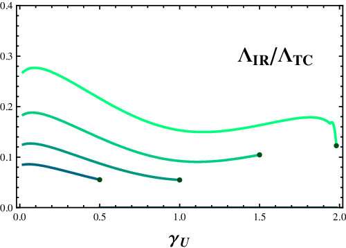
The breaking of scale invariance, due to the coupling to the Higgs sector, was investigated in an earlier reference by the use of naïve dimensional analysis (NDA) [9] . In the appendix B we compare their results with ours. At the parametric level we find,

$$\Lambda_{\rm IR}\gtrsim\Lambda^{\rm NDA}_{\rm IR}\,,$$

(28)

c.f. Fig. 2 (right). The difference being caused by the fact that in the NDA analysis it is implicitly assumed that the unparticle sector scales with the IR cut off whereas in our model the unparticle condensate can also be sensitive to the UV domain. Parametric equality is reached in the region of IR sensitivity, e.g. (1.2). Needless to say that with NDA factors of $4\pi$ can go unnoticed. In connection with the latter a similar criticism could apply to our prescription in (20). Nevertheless it appears to us that it is physically motivated and to some extent is backed up from our empirical knowledge of QCD.

So far we have not specified the normalization factor $B_{d_{\cal U}}$ introduced in Eqs. (10) and (11). In appendix C we motivate the following formula

$$(B_{d_{\cal U}})_{\rm interpol}=2\pi({d_{\cal U}}-1)+\Big(\frac{N_{U}}{16\pi}-\pi\Big)({d_{\cal U}}-1)^{2}\,,$$

(29)

as interpolation formula between the value of $B_{3}$, which is determined by the free fermion loop in our model, and the behaviour around $B_{1}$, which is model independent [36]. As previously stated it differs from the normalization factor $A_{d_{\cal U}}$ in reference [4].

In the next section we will discuss an ETU model in some more detail.

Below the scale $M_{\cal U}$ all four-Fermi interactions have to respect the flavor symmetry $G_{F}$. The most general four-Fermi operators have been classified in [42] and the coefficient of the various operators depend on the specific model used to break the unified gauge theory. Upon Fierz rearrangement, the operators of greatest phenomenological relevance are,

$${\cal L}^{\rm eff}=\Big(\frac{G}{2}\bar{\Psi}_{L}\Sigma\Psi_{R}+{\rm h.c.}\Big)+\frac{G^{\prime}}{2M_{\cal U}^{2}}(\bar{\Psi}_{L}\Psi_{R})(\bar{\Psi}_{R}\Psi_{L})+\dots\ ,$$

(36)

the scalar-scalar interactions of Eq. (4). Here $\Sigma$ is the quark bilinear,

$$\Sigma_{i}^{j}\sim({{Q}_{L}}_{i}{\bar{Q}_{R}^{j}})_{UV}\ ,\qquad i=1,\ldots,F\ .$$

(37)

The flavor indices are contracted and the sum starts from the index value $3$; the first two indices correspond to the $\Psi$’s charged under the electroweak force, which are decoupled at low energy. The fermion bilinear becomes the unparticle operator (7),

$$\big({\cal O_{\cal U}}\big)_{i}^{\;j}=\frac{{{\Psi}_{L}}_{i}\bar{\Psi}_{R}^{j}}{\Lambda_{\cal U}^{\gamma_{\cal U}}}\ .$$

(38)

The matrix $\Sigma$ at energies near the electroweak symmetry breaking scale is identified with the interpolating field for the mesonic composite operators.

To investigate the coupling to the composite Higgs we write down the low energy effective theory using linear realizations. We parameterize the complex $F\times F$ matrix $\Sigma$ by

$$\Sigma=\frac{\sigma+i\,\Theta}{\sqrt{F}}+\sqrt{2}(i\Pi^{a}+\widetilde{\Pi}^{a}){T^{a}}\ ,$$

(39)

where ($\sigma$,$\tilde{\Pi}$) and ($\Theta$,$\Pi$) have $0^{++}$ and $0^{-+}$ quantum numbers respectively. The Lagrangian is given by

	$\displaystyle{\cal L}^{\rm eff}$	$\displaystyle=$	$\displaystyle\frac{1}{2}{\rm Tr}\left[(D\Sigma)^{\dagger}D\Sigma\right]-k_{1}({\rm\widehat{Tr}}\left[\Sigma^{\dagger}\cal O_{\cal U}\right]+{\rm h.c.})-k_{2}{\rm\widehat{Tr}}\left[\cal O_{\cal U}{\cal O_{\cal U}}^{\dagger}\right]$		(40)
			$\displaystyle-m^{2}_{ETC}\sum_{a=4}^{F^{2}-1}\frac{\Pi^{a}\Pi^{a}}{2}-V(\Sigma,\Sigma^{\dagger})\ ,$

where

$\displaystyle D\Sigma=\partial\Sigma-igW\Sigma+ig^{\prime}\Sigma BT^{3}_{R}\ ,\quad{\rm and}\quad W=W^{a}T^{a}_{L}\ ,$

(41)

and ${\rm Tr}[T^{a}_{L/R}T^{b}_{L/R}]=\delta^{ab}/2$. The coefficients $k_{1}$ and $k_{2}$ are directly proportional to the $\alpha^{\prime}$ and $\gamma^{\prime}$ coefficients in (6). The $hat$ on some of the traces indicates that the summation is only on the flavor indices from $3$ to $F$. Three of the Goldstone bosons play the role of the longitudinal gauge bosons and the remaining ones receive a mass $m^{2}_{ETC}$ from an ETC mechanism. We refer the reader to reference [35] for discussion of different ETC models with mechanisms for sufficiently large mass generation. The first term in the Lagrangian is responsible for the mass of the weak gauge bosons and the kinetic term for the remaining Goldstone bosons. The VEV’s for the flavor-diagonal part of the unparticle operator, reduces to the computation performed in the previous section. The potential term preserves the global flavor symmetry $G_{F}$. Up to dimension four, including the determinant responsible for the $\eta^{\prime}$ mass in QCD, the terms respecting the global symmetries of the TC theory are:

$$V(\Sigma,\Sigma^{\dagger})=-\frac{m^{2}}{2}{\rm Tr}\left[\Sigma^{\dagger}\Sigma\right]+\frac{\lambda_{1}}{F}{\rm Tr}\left[\Sigma^{\dagger}\Sigma\right]^{2}+{\lambda_{2}}{\rm Tr}[(\Sigma^{\dagger}\Sigma)^{2}]-\lambda_{3}(\,{\rm det}\Sigma+{\rm det}\Sigma^{\dagger})\ .$$

(42)

The coefficient $m^{2}$ is positive to ensure chiral symmetry breaking in the TC sector. The Higgs VEV enters as follows,

$$\sigma=v+h\ ,\qquad{\rm with}\qquad F_{T}=\sqrt{\frac{2}{F}}\,v\simeq 250\,{\rm GeV}\ .$$

(43)

$F$ here is the number of flavors and $h$ the composite field with the same quantum numbers as the SM Higgs. The particles $\sigma,\Theta,\tilde{\Pi}$ all have masses of the order of $v$. The Higgs mass, the Higgs VEV and the $\Theta$ mass, for instance, are

$\displaystyle v^{2}=\frac{m^{2}}{(\lambda_{1}+\lambda_{2}-\lambda_{3})}\,,\quad m_{h}^{2}=2m^{2}\,,\qquad m_{\Theta}^{2}=4v^{2}\lambda_{3}^{2}\,,$

(44)

up to corrections of the order of $O(\Lambda_{TC}^{2}/{M_{\cal U}^{2}})$ due to contributions from $\alpha$-terms.

The lightest pesudoscalars of the unparticle sector are the pseudo Goldstone bosons emerging from the explicit breaking of the global flavor symmetry in the unparticle sector. Their mass can be read off from the linear term in $O_{\cal U}$ of the effective Largrangian (40)

$$m_{\Pi_{\cal U}}^{2}\simeq\Lambda_{TC}^{2}\left(\frac{\Lambda_{TC}}{{M_{\cal U}^{2}}}\right)^{2}\left(\frac{\Lambda_{\cal U}}{\Lambda_{TC}}\right)^{\gamma_{\cal U}}\left(\frac{\Lambda_{\cal T}}{\Lambda_{TC}}\right)^{\gamma_{\cal T}}\,.$$

(45)

In our model the unparticle propagator to be used for phenomenology, defined from the the Källén-Lehmann representation (A.11), is

$$\Delta_{\cal U}(q^{2},\Lambda_{\rm UV}^{2},\Lambda_{\rm IR}^{2})=-\frac{B_{d_{\cal U}}}{2\pi}\int_{\Lambda_{\rm IR}^{2}}^{\Lambda_{\rm UV}^{2}}\frac{ds\,s^{{d_{\cal U}}-2}}{s-q^{2}-i0}+s.t.\;.$$

(46)

For ${d_{\cal U}}>2$ the integral is sensitive to the UV completion, of which the subtraction terms $(s.t.)$ are a mnemonic. More precisely, the part which is sensitive to $\Lambda_{\rm UV}$ is ambiguous due to the presence of, in principle computable, counterterms, which are expected to be of order one¹²¹² 12 The counterterms are expected to be of order one in a theory which is not fine tuned. This is also known under the term: ’naturalness’. In our model the UV completion is known and the counterterms could in principle be determined, but in practice this is outside the scope of our possibilities.. This will limit, in practice, the predictivity of the theory . Modeling the UV and IR transition regions by hard cut offs is of course a crude model. Yet this should not be relevant as long as $q^{2}$ is sufficiently far away from these cut offs. Whereas, for $q^{2}$ close to the cut off, the integral has an endpoint singularity which is, to a great extent, a model artefact. The situation could be ameliorated for instance by smearing the momentum with a smooth probability density. Due to the breaking of the scale invariance there will be single and multiparticle states appearing in the spectrum, which will affect the $q^{2}\sim\Lambda_{\rm IR}^{2}$ behavior. Having made these statements, we now turn to the evaluation of the integral in (46). It can be expressed as the difference of an IR and UV part,

$$\Delta_{\cal U}(q^{2},\Lambda_{\rm UV}^{2},\Lambda_{\rm IR}^{2})=f_{d_{\cal U}}(\Lambda_{\rm IR}^{2},q^{2}+i0)-f_{d_{\cal U}}(\Lambda_{\rm UV}^{2},q^{2}+i0)\,,$$

(47)

given by,

$$f_{d_{\cal U}}(\Lambda^{2},q^{2})\equiv\Big[\frac{B_{d_{\cal U}}}{2\pi}\frac{(\Lambda^{2})^{{d_{\cal U}}-2}}{{d_{\cal U}}-2}\Big]\underbrace{\!\!\phantom{x}{}_{2}F_{1}(1,2-{d_{\cal U}},3-{d_{\cal U}},\frac{q^{2}}{\Lambda^{2}})}_{\equiv\bar{f}_{d_{\cal U}}(q^{2}/\Lambda^{2})}\,.$$

(48)

For later convenience we give the behaviour of the function $\bar{f}_{d_{\cal U}}(x)$ for small and large argument appropriate for the respective domains:

$$\bar{f}_{d_{\cal U}}(x+i0)=\left\{\begin{array}[]{ll}a_{0}+a_{1}x+O(x^{2})&\quad x\ll 1\quad{\rm UV}\\[2.84544pt] a_{{d_{\cal U}}-2}(-x-i0)^{{d_{\cal U}}-2}+a_{-1}\frac{1}{x}+O(\frac{1}{x^{2}})&\quad x\gg 1\quad{\rm IR}\end{array}\right.\,,$$

(49)

where the leading coefficients are given by

	$\displaystyle a_{0}$	$\displaystyle=1\,,\qquad\qquad\quad$	$\displaystyle a_{-1}$	$\displaystyle=-\frac{\Gamma(1-{d_{\cal U}})\Gamma(3-{d_{\cal U}})}{\Gamma(2-{d_{\cal U}})^{2}}$
	$\displaystyle a_{1}$	$\displaystyle=\frac{{d_{\cal U}}-2}{{d_{\cal U}}-3}\,,\quad$	$\displaystyle a_{{d_{\cal U}}-2}$	$\displaystyle=\Gamma(3-{d_{\cal U}})\Gamma({d_{\cal U}}-1)\,.$		(50)

We shall now turn to the question of the mixing of the unparticle and the Higgs. Our findings resemble results from extra dimensional models. E.g. the model called HEIDI [43], where the continuous spectrum is mimiked by an infinite tower of narrowly spaced Kaluza-Klein modes. The difference is that our model is inherently four dimensional and that the parameters, such as the IR cut off and the strength of the unparticle-Higgs coupling, are related to each other. Our model is also different from the one in reference [10] since, although both are in four dimensions, the Higgs and unparticle coupling emerges dynamically within a UV complete theory.

The interaction term from Eq. (40)

$${\cal L}^{\rm mix}=-g_{h{\cal O}_{\cal U}}\,h{\cal O}_{\cal U}\,,\qquad g_{h{\cal O}_{\cal U}}=\frac{k_{1}(F-2)}{\sqrt{F}}\,,$$

(53)

introduces a mixing between the Higgs and the unparticle. The constant $k_{1}$ has mass dimension $\gamma_{\cal U}$. Its size, on which we will comment below, is crucial for the qualitative nature of the physics. The Higgs propagator is obtained from inverting the combined Higgs-unparticle system

$$\Delta_{hh}(q^{2})=\frac{1}{q^{2}-m_{h}^{2}-g_{h{\cal O}_{\cal U}}^{2}\Delta_{\cal U}(q^{2},\Lambda_{\rm UV}^{2},\Lambda_{\rm IR}^{2})}\,.$$

(54)

This, of course, results in unparticle corrections controlled by $g_{h{\cal O}_{\cal U}}$. The propagator can be rewritten in terms of a dispersion representation

$$\Delta_{hh}(q^{2})=-\int\frac{ds\,\rho_{hh}(s)}{s-q^{2}-i0}\,,$$

(55)

where the density,

$$\int ds\rho_{hh}(s)=1\,,$$

(56)

is automatically normalized to unity. The non zero value of the coupling $g_{h{\cal O}_{\cal U}}$ results solely in a change of basis (or poles and cuts) of the intermediate particles but does not change the overall density of states. A direct way to derive (56) is to equate the representations (55) and (54), multiply them by $q^{2}$ and take the limit $q^{2}\to\infty$ resulting in (56). Please note, this only works in the case where ${d_{\cal U}}<3$, for which the interaction (53) is power counting renormalizable. If this condition is not fulfilled one could resort to a subtracted dispersion relation.

The dispersion representation can be split into resonance¹³¹³ 13 The pole description is only adequate in the narrow width approimation. The Higgs width is of course rather sizable in a theory of strong interactions. The presentation below is meant to be for illustrative purposes only. and continuum contributions,

$$\rho_{hh}(s)=\sum_{i}r_{i}\delta(s-\bar{m}_{i}^{2})+\sigma(s)\,.$$

(57)

The resonance contribution, if present, can then be obtained from the pole equation

$$\Delta_{hh}^{-1}(\bar{m}_{i}^{2})=0\,,\qquad r_{i}=\left|\frac{d\,\Delta_{hh}^{-1}(s)}{ds}\right|^{-1}_{s=\bar{m}_{i}^{2}}\leq 1\,.$$

(58)

The residues $r_{i}$ are smaller (or equal) to one as a consequence of the normalization condition Eq. (56). The continuum is simply given by the cut,

$$\sigma(s)=\Theta(s-\Lambda_{\rm IR}^{2}){\rm Im}[\Delta_{hh}^{-1}(s)]\,,$$

(59)

which corresponds to the imaginary part; most familiar from the optical theorem.

To a large extent the spectral function is characterized by the zeros of the pole equation and the onset of the continuum relative to the poles. This will depend on the strength of the mixing and the anomalous dimension. Somewhat exotic effects can be obtained when the mixing term is made very large [44, 28]¹⁴¹⁴ 14 It should also be mentioned that for very large mixing the theory typically becomes unstable. The pole equation has tachyonic solutions and vertices grow in an uncontrolled manner, indicating the appearance of a new vacuum. It is possible though that interesting effects could arise in a somewhat intermediate regime.. In our model the mixing is determined by $k_{1}$ (53). Its parametric value is given by

$$k_{1}\sim\alpha^{\prime}\Lambda_{TC}^{\gamma_{\cal U}}\left(\frac{\Lambda_{TC}}{{M_{\cal U}}}\right)^{2}\left(\frac{\Lambda_{\cal U}}{\Lambda_{TC}}\right)^{\gamma_{\cal U}}{w_{T}^{\gamma_{\cal T}}}\,,\qquad{w_{T}^{\phantom{x}}}=\left(\frac{\Lambda_{\cal T}}{\Lambda_{TC}}\right)$$

(60)

which we have normalized to the TC scale

The value of $k_{1}$ is, of course, suppressed by the large scale ${M_{\cal U}}$ per se, but receives enhancements from the powers of the anomalous dimensions. For the maximal allowed anomalous dimensions $\gamma_{\cal U}\simeq\gamma_{\cal T}\simeq 2$ and a hierarchy of scales as indicated in the caption of Fig. 2 one finds $k_{1}\Lambda_{TC}^{-\gamma_{\cal U}}\simeq\alpha^{\prime}\cdot O(10^{-2})$. We therefore expect the coupling $g_{h{\cal O}_{\cal U}}\Lambda_{TC}^{-\gamma_{\cal U}}$ (53) to be considerably smaller than one.

In this case there is generally a unique solution to the pole equation. In the IR region $1<{d_{\cal U}}<2$ the analysis can be made quantitative whereas in the UV region $2<{d_{\cal U}}<3$ the uncertainty due to sizable counterterms makes a quantitative assessment difficult. As explained in subsection 2.2.2 these counterterms are expected to be comparable in size only for the leading coefficient $a_{0}$ (49).

At the qualitative level it is an interesting question of whether the Higgs resonance is below or above the threshold [43, 10]. For the values chosen in the caption of Fig. 2 the Higgs resonance is close to the IR cut off. On the other hand it could very well be that the scale ${M_{\cal U}}$ is closer to the GUT scale which would decrease the IR cut off definitely below the composite Higgs mass scale. In appendix D we comment on the unparticle limit of the HEIDI models and compare our parameters with the fit of that model to the excess of the Higgs search at LEP.

References

- [1] S. Weinberg, Phys. Rev. D 19, 1277 (1979).
- [2] L. Susskind, Phys. Rev. D 20, 2619 (1979).
- [3] F. Sannino, arXiv:0804.0182 [hep-ph].
- [4] H. Georgi, Phys. Rev. Lett. 98, 221601 (2007) [arXiv:hep-ph/0703260].
- [5] R. Zwicky, Phys. Rev. D 77, 036004 (2008) [arXiv:0707.0677 [hep-ph]].
- [6] H. Georgi, Phys. Lett. B 650, 275 (2007) [arXiv:0704.2457 [hep-ph]].
- [7] K. Cheung, W. Y. Keung and T. C. Yuan, Phys. Rev. Lett. 99, 051803 (2007) [arXiv:0704.2588 [hep-ph]].
- [8] K. Cheung, W. Y. Keung and T. C. Yuan, arXiv:0809.0995 [hep-ph].
- [9] P. J. Fox, A. Rajaraman and Y. Shirman, Phys. Rev. D 76, 075004 (2007) [arXiv:0705.3092 [hep-ph]].
- [10] A. Delgado, J. R. Espinosa and M. Quiros, JHEP 0710, 094 (2007) [arXiv:0707.4309 [hep-ph]].
- [11] A. Delgado, J. R. Espinosa, J. M. No and M. Quiros, JHEP 0804, 028 (2008) [arXiv:0802.2680 [hep-ph]].
- [12] T. Banks and A. Zaks, Nucl. Phys. B 196, 189 (1982).
- [13] J. Polchinski, Nucl. Phys. B 303, 226 (1988).
- [14] S. Catterall, J. Giedt, F. Sannino and J. Schneible, arXiv:0807.0792 [hep-lat].
- [15] S. Catterall and F. Sannino, Phys. Rev. D 76, 034504 (2007) [arXiv:0705.1664 [hep-lat]].
- [16] L. Del Debbio, M. T. Frandsen, H. Panagopoulos and F. Sannino, JHEP 0806, 007 (2008) [arXiv:0802.0891 [hep-lat]].
- [17] L. Del Debbio, A. Patella and C. Pica, arXiv:0805.2058 [hep-lat].
- [18] Y. Shamir, B. Svetitsky and T. DeGrand, Phys. Rev. D 78, 031502 (2008) [arXiv:0803.1707 [hep-lat]].
- [19] B. Svetitsky, Y. Shamir and T. DeGrand, arXiv:0809.2885 [hep-lat].
- [20] T. DeGrand, Y. Shamir and B. Svetitsky, arXiv:0809.2953 [hep-lat].
- [21] Z. Fodor, K. Holland, J. Kuti, D. Nogradi and C. Schroeder, arXiv:0809.4888 [hep-lat].
- [22] T. Appelquist, G. T. Fleming and E. T. Neil, Phys. Rev. Lett. 100, 171607 (2008) [arXiv:0712.0609 [hep-ph]].
- [23] A. Deuzeman, M. P. Lombardo and E. Pallante, arXiv:0804.2905 [hep-lat].
- [24] Z. Fodor, K. Holland, J. Kuti, D. Nogradi and C. Schroeder, arXiv:0809.4890 [hep-lat].
- [25] T. A. Ryttov and F. Sannino, arXiv:0711.3745 [hep-th].
- [26] T. A. Ryttov and F. Sannino, Phys. Rev. D 76, 105004 (2007) [arXiv:0707.3166 [hep-th]].
- [27] D. D. Dietrich and F. Sannino, Phys. Rev. D 75, 085018 (2007) [arXiv:hep-ph/0611341].
- [28] J. J. van der Bij and S. Dilcher, Phys. Lett. B 655, 183 (2007) [arXiv:0707.1817 [hep-ph]].
- [29] F. Sannino, arXiv:0806.3575 [hep-ph].
- [30] B. Holdom, Phys. Rev. D 24, 1441 (1981).
- [31] T. Appelquist and F. Sannino, Phys. Rev. D 59, 067702 (1999) [arXiv:hep-ph/9806409].
- [32] F. Sannino and K. Tuominen, Phys. Rev. D 71, 051901 (2005) [arXiv:hep-ph/0405209].
- [33] H. Georgi and Y. Kats, arXiv:0805.3953 [hep-ph].
- [34] B. Grinstein, K. A. Intriligator and I. Z. Rothstein, Phys. Lett. B 662, 367 (2008) [arXiv:0801.1140 [hep-ph]].
- [35] C. T. Hill and E. H. Simmons, Phys. Rept. 381, 235 (2003) [Erratum-ibid. 390, 553 (2004)] [arXiv:hep-ph/0203079].
- [36] G. Mack, Commun. Math. Phys. 55, 1 (1977).
- [37] R. Foadi, M. T. Frandsen, T. A. Ryttov and F. Sannino, Phys. Rev. D 76, 055005 (2007) [arXiv:0706.1696 [hep-ph]].
- [38] D. K. Hong, S. D. H. Hsu and F. Sannino, Phys. Lett. B 597, 89 (2004) [arXiv:hep-ph/0406200].
- [39] M. A. Stephanov, Phys. Rev. D 76, 035008 (2007) [arXiv:0705.3049 [hep-ph]].
- [40] H. D. Politzer, Nucl. Phys. B 117, 397 (1976).
- [41] T. Appelquist, K. D. Lane and U. Mahanta, Phys. Rev. Lett. 61, 1553 (1988).
- [42] T. Appelquist, M. J. Bowick, E. Cohler and A. I. Hauser, Phys. Rev. D 31, 1676 (1985).
- [43] J. J. van der Bij and S. Dilcher, Phys. Lett. B 638, 234 (2006) [arXiv:hep-ph/0605008].
- [44] A. Delgado, J. R. Espinosa, J. M. No and M. Quiros, arXiv:0804.4574 [hep-ph].
- [45] D. Stancato and J. Terning, arXiv:0807.3961 [hep-ph].
- [46] X. Calmet, N. G. Deshpande, X. G. He and S. D. H. Hsu, arXiv:0810.2155 [hep-ph].
- [47] A. Belyaev, R. Foadi, M. T. Frandsen, M. Jarvinen, F. Sannino and A. Pukhov, arXiv:0809.0793 [hep-ph].
- [48] A. R. Zerwekh, Eur. Phys. J. C 46, 791 (2006) [arXiv:hep-ph/0512261].
- [49] K. Agashe, S. Gopalakrishna, T. Han, G. Y. Huang and A. Soni, arXiv:0810.1497 [hep-ph].
- [50] D. D. Dietrich, F. Sannino and K. Tuominen, Phys. Rev. D 72, 055001 (2005) [arXiv:hep-ph/0505059].
- [51] N. D. Christensen and R. Shrock, Phys. Rev. D 74, 015004 (2006) [arXiv:hep-ph/0603149].
- [52] N. D. Christensen and R. Shrock, Phys. Rev. D 72, 035013 (2005) [arXiv:hep-ph/0506155].
- [53] T. Appelquist and R. Shrock, AIP Conf. Proc. 721, 261 (2004).
- [54] T. Appelquist, N. D. Christensen, M. Piai and R. Shrock, Phys. Rev. D 70, 093010 (2004) [arXiv:hep-ph/0409035].
- [55] T. Appelquist, M. Piai and R. Shrock, Phys. Rev. D 69, 015002 (2004) [arXiv:hep-ph/0308061].
- [56] T. Appelquist and R. Shrock, Phys. Rev. Lett. 90, 201801 (2003) [arXiv:hep-ph/0301108].
- [57] S. B. Gudnason, T. A. Ryttov and F. Sannino, Phys. Rev. D 76, 015005 (2007) [arXiv:hep-ph/0612230].
- [58] M. Pospelov, A. Ritz and M. B. Voloshin, Phys. Lett. B 662, 53 (2008) [arXiv:0711.4866 [hep-ph]].
- [59] T. Kikuchi and N. Okada, Phys. Lett. B 665, 186 (2008) [arXiv:0711.1506 [hep-ph]].
- [60] Y. Nambu and G. Jona-Lasinio, Phys. Rev. 122, 345 (1961).