An accurate analytic description of neutrino oscillations in matter
Abstract
A simple closed-form analytic expression for the probability of two-flavour neutrino oscillations in a matter with an arbitrary density profile is derived. Our formula is based on a perturbative expansion and allows an easy calculation of higher order corrections. The expansion parameter is small when the density changes relatively slowly along the neutrino path and/or neutrino energy is not very close to the Mikheyev-Smirnov-Wolfenstein (MSW) resonance energy. Our approximation is not equivalent to the adiabatic approximation and actually goes beyond it. We demonstrate the validity of our results using a few model density profiles, including the PREM density profile of the Earth. It is shown that by combining the results obtained from the expansions valid below and above the MSW resonance one can obtain a very good description of neutrino oscillations in matter in the entire energy range, including the resonance region.
1 Introduction
In most neutrino oscillation experiments neutrinos propagate substantial distances in matter before reaching a detector, and therefore an accurate description of neutrino oscillations in matter [1, 2] is an important ingredient of the analyses of the data. For a matter of an arbitrary density profile the neutrino evolution equation admits no closed-form solution, and one usually has to resort to numerical methods. While numerical integration of the evolution equation usually poses no problem, it is still highly desirable to have approximate analytic solutions, which may provide a significant insight into the physics of neutrino oscillations in matter, clarify the dependence of the oscillation probabilities on the neutrino parameters and in many cases help save the CPU time. To this end, a number of analytic solutions of the neutrino evolution equation in matter, based on various approximations, has been developed (for recent studies, see e.g. [3, 4, 5, 6, 7, 8, 9, 10]).
In this paper we derive a simple analytic expression for the two-flavour oscillation probability valid for an arbitrary matter density profile. We employ a perturbative approach based on the expansion in a parameter which is small when the density changes relatively slowly along the neutrino path and/or neutrino energy is not very close to the Mikheyev-Smirnov-Wolfenstein (MSW) [1, 2] resonance energy. Our approximation is not equivalent to the adiabatic approximation and actually goes beyond it. We demonstrate the validity of our results using a few model density profiles, including the important PREM profile [11], which gives a realistic description of matter density distribution inside the Earth. We also show that, by combining the results obtained for the energies below and above the MSW resonance ones, one can obtain an excellent description of neutrino oscillations in matter in the entire energy range. The simple form of our result and the wide range of its applicability are the two main advantages of this approach.
An approach similar to ours has been employed in [12, 7]. Unlike in those publications, in the present work we do not confine ourselves to the leading approximation, but also calculate the first and second order corrections and show that this improves the accuracy of the approximation drastically.
The paper is organized as follows. In Sec. 2 we present the formalism used to derive our analytic solution. In Sec. 3 we apply this method to the case of a parabolic and a power law matter potentials. In Sec. 4 we present the results obtained in the case of the realistic PREM Earth’s density profile. We discuss our results and conclude in Sec. 5.
2 The formalism
In a number of important cases the full three-flavour neutrino oscillations can to a very good accuracy be reduced to effective two-flavour ones. These include oscillations either in the limit of vanishingly small 1-3 mixing, when the oscillations are essentially driven by the “solar” parameters and , or at sufficiently high energies ( GeV for oscillations in the Earth), when the 1-2 mixing in matter is strongly suppressed; in that case the oscillation probabilities are essentially independent of the “solar” parameters and are governed by and . For definiteness, in our numerical examples we will concentrate on the second case, though our general discussion will be valid in both situations.
Two-flavour oscillations of neutrinos in matter are described by the Schrödinger-like evolution equation [1, 2]
| (1) |
where the overdot denotes the differentiation with respect to the coordinate, and and are respectively the probability amplitudes to find and , the latter being a linear combination of and . In the limit when the 1-3 mixing vanishes, , one has , whereas in the situations when the solar parameters play practically no role (e.g. for oscillations of high-energy neutrinos in the Earth), . The quantities and in Eq. (1) are
| (2) |
Here the function depends on the electron number density through the Wolfenstein potential defined as
where is the Fermi constant, is the mass density of matter and is the number of electrons per nucleon. The parameter is defined as , and is the relevant mixing angle in vacuum. In the limit one has , , and the oscillation probabilities are given by
| (3) |
| (4) |
Here is the effective two-flavour oscillation probability:
| (5) |
(we assume the initial conditions , ). For oscillations of high-energy neutrinos in the Earth one has , , and the oscillation probabilities are
| (6) |
| (7) |
where, as before, is given by Eq. (5).
Differentiating Eq. (1), one can find decoupled second order differential equations for and [13, 14]. The equation for the transition amplitude reads
| (8) |
where we have defined the function as
| (9) |
Note that the instantaneous eigenvalues of the effective Hamiltonian in Eq. (1) are . The equation for differs from Eq. (8) by the sign of the term.
It will be convenient for our purposes to rewrite Eq. (8) in the following form:
| (10) |
where we have introduced the notation
| (11) |
Eq. (10) cannot in general be solved exactly, but, as we shall see, it admits a simple perturbative solution. To show that, let us first notice that, for energies (or densities) above the MSW resonance one, the quantity on the right hand side of Eq. (10) is small. Indeed, from Eqs. (9) and (2) it follows that for (i.e. for ) one has , so that . The smallness of the parameter allows one to solve Eq. (10) perturbatively, order by order. Expanding in powers of , we find the equation for the th order transition amplitude (with ):
| (12) |
The zero order transition amplitude satisfies the equation with the vanishing right hand side:
| (13) |
Its solution for an arbitrary functional dependence of on the coordinate can be readily found by considering the quantity , which, as follows from (13), satisfies the first-order equation . Taking into account that the initial conditions , also imply, through Eq. (1), , one finds
| (14) |
where
| (15) |
This yields the zero-order solution for the two-flavour transition probability [12, 7]:
| (16) |
Assuming that the amplitude on the right hand side of Eq. (12) is known, one can solve it for . To this end, we introduce the quantity
| (17) |
in terms of which Eq. (12) can be rewritten as
| (18) |
This can now be solved by the standard methods. First, we find the general solution of the homogeneous equation
| (19) |
which gives
| (20) |
with an integration constant. Next, the solution of the inhomogenous equation (18) is found by allowing to depend on the coordinate and substituting Eq. (20) back into Eq. (18). Taking into account the initial condition , one finds
| (21) |
The solution for is now given by Eq. (20) with replaced by from Eq. (21). Once is known, it is straightforward to solve Eq. (17) for . This yields
| (22) |
where we have used Eq. (14). The corresponding th order effective two-flavour oscillation probability is then found as .
Eq. (22) represents the main result of our paper. It gives an analytic expression for the oscillation amplitude in the th order in perturbation theory in terms of the lower-order solutions and . For our numerical illustrations we will consider the solutions with , 1 and 2.
Eq. (22) has been derived under the assumption that is a small parameter. As we pointed out before, this is true for energies above the MSW resonance one. This means that the perturbative approach considered above should, in general, fail for energies below the MSW resonance one. However, a simple modification of the above procedure leads to a description of neutrino oscillations valid below the MSW resonance. In order to show this, let us, instead of casting Eq. (8) in the form (10), rewrite it as
| (23) |
where is now defined as
| (24) |
For small vacuum mixing angles, this is a small parameter below the MSW resonance, since in that case and so . Therefore, we can proceed with the perturbative approach, as before. Comparing Eqs. (23) and (24) with Eqs. (10) and (11) respectively, we see that the two pairs of equations differ only by the sign of . Therefore the solution of Eq. (23) can be obtained from Eq. (22) by simply replacing by . This will also change the values of the oscillation probabilities obtained in all orders in perturbation theory except for the zero-order probability which, as can be seen from (16), is invariant with respect to the flip of the sign of . As we shall see, by combining the results valid above and below the MSW resonance one can obtain a very good description of neutrino oscillations in matter in the entire energy range.
Let us now discuss the expansion parameter of our perturbative approach. We have found that the corrections to the zero order amplitude are proportional to , where the upper and lower signs refer to the energies above and below the MSW resonance, respectively. These quantities can be expressed through the mixing angle in matter :11 1 Note that , .
| (25) |
Far above the MSW resonance one has , whereas far below the resonance , which is close to 1 in the case of small vacuum mixing. This demonstrates the smallness of in its corresponding domains of validity. At the MSW resonance one has , and is only small if is.
An examination of Eq. (22) shows that the expansion parameter of our perturbative approach is actually (see Eq. (15)). In various energy domains we have
| (26) |
where we have used the shorthand notation , . From Eq. (26) it is easy to see that outside the MSW resonance region the expansion parameter approximately satisfies
| (27) |
where is the MSW adiabaticity parameter. Thus, for small mixing in matter () our approximation is better than the adiabatic one. Close to the resonance the two approaches have comparable accuracy.
3 Two examples: parabolic and power law profiles
As a first study, we apply our formalism to two simple density distributions: a parabolic and a power law profile.
For the parabolic profile, we consider the following density distribution:
| (28) |
with
| (29) |
and we take the baseline to be km. Note that the parabolic density profile represents a good approximation for the density distribution felt by neutrinos in the Earth when they cross only the Earth’s mantle.
Next, we analyze the case of the following power-law density distribution:
| (30) |
with
| (31) |
and we consider neutrino propagation over the distance km. The profile represents a realistic description of the density distribution inside supernovae; note, however, that neutrino flavour transitions in supernovae are more adequately described by different methods (see, e.g., [15]), and so we consider the profile (30) just for illustration.
The results based on our perturbative analytic approach for the profiles (28) and (30) are presented in Fig. 1, where they are compared with the exact ones, obtained by direct numerical integration of the neutrino evolution equation (1). The upper panels show the oscillation probabilities for the parabolic density profile and the lower ones, for the power-law profile (30). The left panels correspond to the expansion valid for energies below the MSW resonance ones, whereas the right panels were obtained for the expansion valid above the resonance energies. As expected, the zero-order approximation gives a good accuracy only outside the MSW resonance region (i.e., outside the intervals – 6 GeV for the parabolic profile and 30 -- 50 MeV for the power-law one).22 2 Note that, since the profiles (28) and (30) (as well as the PREM profile considered in the next section) span a range of matter densities, neutrinos in an interval of energies experience the MSW resonance. The first-order perturbative results obtained using the expansion valid below the MSW resonance extend slightly the region of good accuracy towards higher energies, closer to the MSW resonance, though in general fail for energies above the MSW resonance, whereas the first-order results found from the expansion valid above the MSW resonance extend the region of good accuracy to lower energies, but in general fail below the MSW resonance. Thus, the first-order calculation taken in their respective domains of applicability allow to achieve a good description of the exact results closer to the resonance energy than the zero-order solutions do, i.e. they reduce the energy domain in which the approximation fails. At the same time, as can be seen from Fig. 1, the second-order probabilities practically coincide with the corresponding exact results, irrespectively of whether they are obtained using the expansion valid below or above the MSW resonance.
4 Propagation inside the Earth: PREM profile
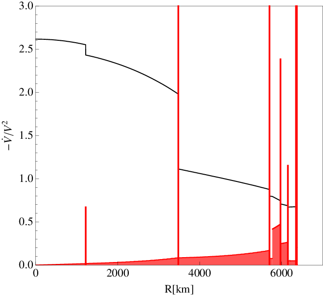
Neutrinos coming from various sources can propagate inside the Earth before reaching a detector. Examples are atmospheric neutrinos, neutrinos coming from WIMP annihilation inside the Earth or the Sun, as well as neutrinos studied in long-baseline accelerator experiments. We will consider here oscillations of high-energy neutrinos in the Earth, for which we take the matter density distribution as described by the PREM profile [11] (Fig. 3). Note that the PREM profile is symmetric with respect to the midpoint of the neutrino trajectory, and therefore the two-flavour transition amplitude obtained as a solution of Eq. (1) is pure imaginary due to the time reversal symmetry of the problem [16].
In Fig. 2 we present the oscillation probability as a function of neutrino energy for two values of the zenith angle of the neutrino trajectory: , when the neutrinos propagate the longest distance inside the Earth, traversing it along its diameter, and , when they do not cross the inner core of the Earth. As in Fig. 1, we compare the approximate solutions, up to the second order (), with the exact solutions found by direct numerical integration of the neutrino evolution equation. In this figure (as well as in Figs. 4 – 6 below) in the left panels we present the oscillation probabilities obtained with the expansion valid below the MSW resonance energy, whereas the right panels show the results found from the expansion valid above the MSW resonance.
It can be seen from Fig. 2 that the zero order probability reproduces accurately the exact one, , only for energies that are outside the resonance region. Indeed, the two solutions nearly coincide for 2.5 GeV and for GeV, but deviate substantially between these energies. As can be seen from the figure, the accuracy of the first order solutions is slightly better in their respective domain of validity: the solutions valid below the resonance (left panels of the figure) allow an accurate description of the probability for slightly higher energies than does, allowing to come closer to the MSW resonance from below; however, they fail badly (not even being bounded by 1) above the resonance. Likewise, the solutions valid above the resonance (right panels) allow to come closer to the MSW resonance from above, but fail below the resonance.
At the same time, the second-order solution gives quite a good approximation to the exact probability for all energies, though the solutions obtained through the expansions in their corresponding domains of validity give a better accuracy in these energy domains. By combining the second-order solutions valid below and above the MSW resonance, one can obtain a very good description of the exact oscillation probability practically at all energies, including the resonance region. We have also checked that for trajectories that do not cross the core of the Earth ( -0.838), for which the matter density profile seen by the neutrinos is relatively smooth, the second order solutions obtained through both expansions essentially coincide with the exact one for all energies.
In Fig. 4 we present the oscillation probability , obtained in different orders in perturbation theory, as a function of the distance travelled by neutrinos inside the Earth for vertically up-going neutrinos () and two values of neutrino energy, GeV and 6 GeV. The figure clearly demonstrates how the accuracy improves with increasing order in perturbation theory; the second order solutions nearly concide with the exact probability along the entire neutrino path.
Fig. 5 illustrates the dependence of the analytic solutions on the zenith angle for two values of the neutrino energy, GeV and 6 GeV. For both energies we show the solutions obtained using the expansions valid below and above the MSW resonance. The results agree with our expectations: the second order solution based on the expansion valid below the resonance reproduces the exact one extremely well for GeV but does not give a good accuracy (especially in the core region) for GeV, while the situation is opposite in the case of the solution corresponding to the expansion valid above the resonance.
Finally, in Fig. 6 we show the dependence of the accuracy of the analytic solutions on the value of the vacuum mixing angle . As one can see by comparing the upper panels with the corresponding lower ones, with decreasing value of the accuracy of our perturbative expansion improves. This is the consequence of the fact that the expansion parameter (27) decreases with decreasing .
5 Discussion and conclusions
We have developed a perturbative approach for two-flavour neutrino oscillations in matter with an arbitrary density profile. The zero-order oscillation amplitude satisfies the equation which can be solved analytically for an arbitrary dependence of the matter density distribution on the coordinate along the neutrino path; higher order amplitudes are then obtained from the lower-order ones through a simple perturabative procedure. We have studied the zeroth, first and second order solutions and compared them with each other and with the exact oscillation probability obtained by numerical integration of the neutrino evolution equation. In all orders except the zeroth one, the expansion scheme depends on whether the neutrino energy is above or below the MSW resonance energy, and one has to consider these two cases separately.
While the zero-order result gives a very good accuracy outside the resonance region, higher order corrections are necessary to achieve an accurate description of the oscillation probability in the vicinity of the MSW resonance. We have demonstrated how these corrections, when taken in their respective energy domains of validity, improve drastically the precision of the approximation.
For the smooth density profiles that we have studied, we found that the second order oscillation probability reproduces the exact one extremely well in the whole interval of energies, including the MSW resonance region, independently of whether the expansion scheme valid below or above the resonance was used. The same is also true for the PREM density profiles in the case when neutrinos cross only the mantle of the Earth, since the density jumps experienced by neutrinos in that case are relatively small. The high accuracy of the second order approximation for smooth density profiles is related to the fact that our expansion parameter, Eq. (27), is proportional to . This parameter is smaller than the expansion parameter of the adiabatic approximation by the factor and therefore our approach gives a better accuracy than the adiabatic expansion when the mixing in matter is small. Note that a different expansion of the same evolution equation (8) was employed in [17].
For energies above the MSW resonance, our expansion parameter is essentially
| (32) |
For the PREM density profile of the Earth, the function is plotted in the right panel of Fig. 3. As can be seen from the figure, in most of the coordinate space the value of this function does not exceed 0.25. The spikes corresponding to the density jumps, though quite high, are very narrow; they do not destroy our approximation because their contributions get suppressed due to the integrations involved in the calculation of the higher-order corrections to the oscillation amplitude (see Eq. (22)). Still, these contributions are not negligible, especially for neutrinos crossing the Earth’s core. As a result, for core-crossing neutrinos with energies close to the MSW resonance ones, even the second-order oscillation probabilities are only adequate when taken in their respective energy domains of validity. By combining the solutions valid below and above the MSW resonance one obtains a very accurate description of neutrino oscillations in matter in the entire energy range.
To conclude, we have derived a simple closed-form analytic expression for the probability of two-flavour neutrino oscillations in a matter with an arbitrary density profile. Our formula is based on a perturbative expansion and allows an easy calculation of higher order corrections. We have applied our formalism to a number of density distributions, including the PREM density profile of the Earth, and demonstrated that the second-order approximation gives a very good accuracy in the entire energy interval.
Acknowledgments
We thank Andreas Hohenegger for the help with numerical calculations and Michele Maltoni for useful discussions.
References
- [1] L. Wolfenstein, Phys. Rev. D17, 2369 (1978).
- [2] S. P. Mikheev and A. Y. Smirnov, Sov. J. Nucl. Phys. 42, 913 (1985).
- [3] P. C. de Holanda, W. Liao, and A. Y. Smirnov, Nucl. Phys. B702, 307 (2004), arXiv: hep-ph/0404042 .
- [4] A. N. Ioannisian and A. Y. Smirnov, Phys. Rev. Lett. 93, 241801 (2004), arXiv: hep-ph/0404060 .
- [5] E. K. Akhmedov, M. A. Tortola, and J. W. F. Valle, JHEP 05, 057 (2004), arXiv: hep-ph/0404083 .
- [6] A. N. Ioannisian, N. A. Kazarian, A. Y. Smirnov, and D. Wyler, Phys. Rev. D71, 033006 (2005), arXiv: hep-ph/0407138 .
- [7] E. K. Akhmedov, M. Maltoni, and A. Y. Smirnov, Phys. Rev. Lett. 95, 211801 (2005), arXiv: hep-ph/0506064 .
- [8] W. Liao, Phys. Rev. D77, 053002 (2008), arXiv: 0710.1492 .
- [9] A. D. Supanitsky, J. C. D’Olivo, and G. Medina-Tanco (2007), arXiv: 0708.0629 .
- [10] A. N. Ioannisian and A. Y. Smirnov (2008), arXiv: 0803.1967 .
- [11] A. M. Dziewonski and D. L. Anderson, Phys. Earth Planet. Interiors 25, 297 (1981).
- [12] E. K. Akhmedov, Sov. J. Nucl. Phys. 47, 301 (1988).
- [13] V. K. Ermilova, V. A. Tsarev, and V. A. Chechin, JETP Lett. 43, 453 (1986).
- [14] D. Notzold, Phys. Rev. D36, 1625 (1987).
- [15] A. S. Dighe and A. Y. Smirnov, Phys. Rev. D62, 033007 (2000), arXiv: hep-ph/9907423 .
- [16] E. K. Akhmedov, P. Huber, M. Lindner, and T. Ohlsson, Nucl. Phys. B608, 394 (2001), arXiv: hep-ph/0105029 .
- [17] A. B. Balantekin, S. H. Fricke, and P. J. Hatchell, Phys. Rev. D38, 935 (1988).
 |
 |
 |
 |
 |
 |
 |
 |
 |
 |
 |
 |
 |
 |
 |
 |
 |
 |
 |
 |