Dissections, orientations, and trees,
with applications to
optimal mesh encoding
and to random sampling
Abstract
We present a bijection between some quadrangular dissections of an hexagon and unrooted binary trees, with interesting consequences for enumeration, mesh compression and graph sampling. Our bijection yields an efficient uniform random sampler for 3-connected planar graphs, which turns out to be determinant for the quadratic complexity of the current best known uniform random sampler for labelled planar graphs [Fusy, Analysis of Algorithms 2005]. It also provides an encoding for the set of -edge 3-connected planar graphs that matches the entropy bound bits per edge (bpe). This solves a theoretical problem recently raised in mesh compression, as these graphs abstract the combinatorial part of meshes with spherical topology. We also achieve the optimal parametric rate bpe for graphs of with vertices and faces, matching in particular the optimal rate for triangulations. Our encoding relies on a linear time algorithm to compute an orientation associated to the minimal Schnyder wood of a 3-connected planar map. This algorithm is of independent interest, and it is for instance a key ingredient in a recent straight line drawing algorithm for 3-connected planar graphs [Bonichon et al., Graph Drawing 2005].
Keywords:
Algorithmscategory
G.2.1 Discrete Mathematics Combinatorial algorithmskeywords
Bijection, Counting, Coding, Random generation1 Introduction
One origin of this work can be traced back to an article of Ed Bender in the American Mathematical Monthly [4], where he asked for a simple explanation of the remarkable asymptotic formula
| (1) |
for the cardinality of the set of 3-connected (unlabelled) planar graphs with vertices, faces and edges, going to infinity. By a theorem of \citeNWhitney33, these graphs have essentially a unique embedding on the sphere up to homeomorphisms, so that their study amounts to that of rooted 3-connected maps, where a map is a graph embedded in the plane and rooted means with a marked oriented edge.
1.1 Graphs, dissections and trees
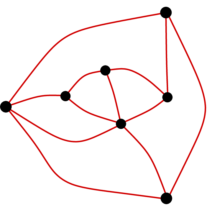
Another known property of 3-connected planar graphs with edges is the fact that they are in direct one-to-one correspondence with dissections of the sphere into quadrangles that have no non-facial 4-cycle. The heart of our paper lies in a further one-to-one correspondence.
Theorem 1.1
There is a one-to-one correspondence between unrooted binary trees with nodes and unrooted quadrangular dissections of an hexagon with interior vertices and no non-facial 4-cycle.
The mapping from binary trees to dissections, which we call the closure, is easily described and resembles constructions that were recently proposed for simpler kinds of maps [37, 8, 35]. The proof that the mapping is a bijection is instead rather sophisticated, relying on new properties of constrained orientations [33], related to Schnyder woods of triangulations and 3-connected planar maps [39, 3, 16] .
Conversely, the reconstruction of the tree from the dissection relies on a linear time algorithm to compute the minimal Schnyder woods of a 3-connected map (or equivalently, the minimal -orientation of the associated derived map, see Section 9). This problem is of independant interest and our algorithm has for example applications in the graph drawing context [6]. It is akin to Kant’s canonical ordering [25, 13, 7, 11], but again the proof of correctness is quite involved.
Theorem 1.1 leads directly to the implicit representation of the numbers —counting rooted 3-connected maps with edges— due to \citeNTu63), and its refinement as discussed in Section 5 yields that of the number of rooted 3-connected maps with vertices and faces (due to \citeNMu) from which Formula (1) follows. It partially explains the combinatorics of the occurrence of the cross product of binomials, since these are typical of binary tree enumerations. Let us mention that the one-to-one correspondence specializes particularly nicely to count plane triangulations (i.e., 3-connected maps with all faces of degree 3), leading to the first bijective derivation of the counting formula for unrooted plane triangulations with vertices, originally found by \citeNBr using algebraic methods.
1.2 Random sampling
A second byproduct of Theorem 1.1 is an efficient uniform random sampler for rooted 3-connected maps, i.e., an algorithm that, given , outputs a random element in the set of rooted 3-connected maps with edges with equal chances for all elements. The same principles yield a uniform sampler for .
The uniform random generation of classes of maps like triangulations or 3-connected graphs was first considered in mathematical physics (see references in [2, 35]), and various types of random planar graphs are commonly used for testing graph drawing algorithms (see \citeAtaxiplan).
The best previously known algorithm [38] had expected complexity for , and was much less efficient for , having even exponential complexity for or tending to 2 (due to Euler’s formula these ratio are bounded above by 2 for 3-connected maps). In Section 6, we show that our generator for or performs in linear time except if or tends to 2 where it becomes at most cubic.
From the theoretical point of view, it is also desirable to work with the uniform distribution on planar graphs. However, random (labelled) planar graphs appear to be challenging mathematical objects [34, 29]. A Markov chain converging to the uniform distribution on planar graphs with vertices was given by \citeNDVW96, but it resists known approaches for perfect sampling [45], and has unknown mixing time. As opposed to this, a recursive scheme to sample planar graphs was proposed by \citeNBGK03, with amortized complexity . This result is based on a recursive decomposition of planar graphs: a planar graph can be decomposed into a tree-structure whose nodes are occupied by rooted 3-connected maps. Generating a planar graph reduces to computing branching probabilities so as to generate the decomposition tree with suitable probability; then a random rooted 3-connected map is generated for each node of the decomposition tree. \citeNBGK03 use the so-called recursive method [32, 18, 44] to take advantage of the recursive decomposition of planar graphs. Our new random generator for rooted 3-connected maps reduces their amortized cost to . Finally a new uniform random generator for planar graphs was recently developped by one of the authors [20], that avoids the expensive preprocessing computations of [5]. The recursive scheme is similar to the one used in [5], but the method to translate it to a random generator relies on Boltzmann samplers, a new general framework for the random generation recently developed in [15]. Thanks to our random generator for rooted 3-connected maps, the algorithm of [20] has a time-complexity of for exact size uniform sampling and even performs in linear time for approximate size uniform sampling.
1.3 Succinct encoding
A third byproduct of Theorem 1.1 is the possibility to encode in linear time a 3-connected planar graph with edges by a binary tree with nodes. In turn the tree can be encoded by a balanced parenthesis word of bits. This code is optimal in the information theoretic sense: the entropy per edge of this class of graphs, i.e., the quantity , tends to 2 when goes to infinity, so that a code for cannot give a better guarantee on the compression rate.
Applications calling for compact storage and fast transmission of 3D geometrical meshes have recently motivated a huge literature on compression, in particular for the combinatorial part of the meshes. The first compression algorithms dealt only with triangular faces [36, 40], but many meshes include larger faces, so that polygonal meshes have become prominent (see [1] for a recent survey).
The question of optimality of coders was raised in relation with exception codes produced by several heuristics when dealing with meshes with spherical topology [22, 26]. Since these meshes are exactly triangulations (for triangular meshes) and 3-connected planar graphs (for polyhedral ones), the coders in [35] and in the present paper respectively prove that traversal based algorithms can achieve optimality.
On the other hand, in the context of succinct data structures, almost optimal algorithms have been proposed [24, 28], that are based on separator theorems. However these algorithms are not truly optimal (they get close to the entropy but at the cost of an uncontrolled increase of the constants in the linear complexity). Moreover, although they rely on a sophisticated recursive structure, they do not support efficient adjacency requests.
As opposed to that, our algorithm shares with [23, 7] the property that it produces essentially the code of a spanning tree. More precisely it is just the balanced parenthesis code of a binary tree, and adjacencies of the initial dissection that are not present in the tree can be recovered from the code by a simple variation on the interpretation of the symbols. Adjacency queries can thus be dealt with in time proportional to the degree of vertices [12] using the approach of [31, 23].
Finally we show that the code can be modified to be optimal on the class . Since the entropy of this class is strictly smaller than that of as soon as , the resulting parametric coder is more efficient in this range. In particular in the case our new algorithm specializes to an optimal coder for triangulations.
1.4 Outline of the paper
The paper starts with two sections of preliminaries: definitions of the maps and trees involved (Section 2), and some basic correspondences between them (Section 3). Then comes our main result (Section 4), the mapping between binary trees and some dissections of the hexagon by quadrangular faces. The fact that this mapping is a bijection follows from the existence and uniqueness of a certain tri-orientation of our dissections. The proof of this auxiliary theorem, which requires the introduction of the so-called derived maps and their -orientations, is delayed to Section 8, that is, after the three sections dedicated to applications of our main result: in these sections we successively discuss counting (Section 5), sampling (Section 6) and coding (Section 7) rooted 3-connected maps. The third application leads us to our second important result: in Section 9 we present a linear time algorithm to compute the minimal -orientation of the derived map of a 3-connected planar map (which also corresponds to the minimal Schnyder woods alluded to above). Finally, Section 10 is dedicated to the correctness proof of this orientation algorithm. Figure 1 summarizes the connections between the different families of objects we consider.
0,-3)(20,14) iterative algorithm transposition operations 0)opening 1)closure rejection Whitney folklore
2 Definitions
2.1 Planar maps
A planar map is a proper embedding of an unlabelled connected graph in the plane, where proper means that edges are smooth simple arcs that do not meet but at their endpoints. A planar map is said to be rooted if one edge of the outer face, called the root-edge, is marked and oriented such that the outer face lays on its right. The origin of the root-edge is called root-vertex. Vertices and edges are said to be outer or inner depending on whether they are incident to the outer face or not.
A planar map is 3-connected if it has at least 4 edges and can not be disconnected by the removal of two vertices. The first 3-connected planar map is the tetrahedron, which has 6 edges. We denote by (respectively ) the set of rooted 3-connected planar maps with edges (resp. vertices and faces). A 3-connected planar map is outer-triangular if its outer face is triangular.
2.2 Plane trees, and half-edges
Plane trees are planar maps with a single face —the outer one. A vertex is called a leaf if it has degree 1, and node otherwise. Edges incident to a leaf are called stems, and the other are called entire edges. Observe that plane trees are unrooted trees.
Binary trees are plane trees whose nodes have degree 3. By convention we shall require that a rooted binary tree has a root-edge that is a stem. The root-edge of a rooted binary tree thus connects a node, called the root-node, to a leaf, called the root-leaf. With this definition of rooted binary tree, upon drawing the tree in a top down manner starting with the root-leaf, every node (including the root-node) has a father, a left son and a right son. This (very minor) variation on the usual definition of rooted binary trees will be convenient later on. For , we denote respectively by and the sets of binary and rooted binary trees with nodes (they have leaves, as proved by induction on ). These rooted trees are well known to be counted by the Catalan numbers: .
The vertices of a binary tree can be greedily bicolored —say in black or white— so that adjacent vertices have distinct colors. The bicoloration is unique up to the choice of the color of the first node. As a consequence, rooted bicolored binary trees are either black-rooted or white-rooted, depending on the color of the root node. The sets of black-rooted (resp. white-rooted) binary trees with black nodes and white nodes is denoted by (resp. by ); and the total set of rooted bicolored binary trees with black nodes and white nodes is denoted by .
It will be convenient to view each entire edge of a tree as a pair of opposite half-edges —each one incident to one extremity of the edge— and to view each stem as a single half-edge —incident to the node holding the stem. More generally we shall consider maps that have entire edges (made of two half-edges) and stems (made of only one half-edge). It is then also natural to associate one face to each half-edge, say, the face on its right. In the case of trees, there is only the outer face, so that all half-edges get the same associated face.
2.3 Quadrangulations and dissections
A quadrangulation is a planar map whose faces (including the outer one) have degree 4. A dissection of the hexagon by quadrangular faces is a planar map whose outer face has degree 6 and inner faces have degree 4.
Cycles that do not delimit a face are said to be separating. A quadrangulation or a dissection of the hexagon by quadrangular faces is said to be irreducible if it has at least 4 faces and has no separating 4-cycle. The first irreducible quadrangulation is the cube, which has 6 faces. We denote by the set of rooted irreducible quadrangulations with faces, including the outer one. Euler’s relation ensures that these quadrangulations have vertices. We denote by () the set of (rooted, respectively) irreducible dissections of the hexagon with inner vertices. These have quadrangular faces, according to Euler’s relation. From now on, irreducible dissections of the hexagon by quadrangular faces will simply be called irreducible dissections. The classes of rooted irreducible quadrangulations and of rooted irreducible dissections are respectively denoted by and .
As faces of dissections and quadrangulations have even degree, the vertices of these maps can be greedily bicolored, say, in black and white, so that each edge connects a black vertex to a white one. Such a bicoloration is unique up to the choice of the colors. We denote by the set of rooted bicolored irreducible quadrangulations with black vertices and white vertices and such that the root-vertex is black; and by the set of rooted bicolored irreducible dissections with black inner vertices and white inner vertices and such that the root-vertex is black.
A bicolored irreducible dissection is complete if the three outer white vertices of the hexagon have degree exactly 2. Hence, these three vertices are incident to two adjacent edges on the hexagon.
3 Correspondences between families of planar maps
This section recalls a folklore bijection between irreducible quadrangulations and 3-connected maps, hereafter called angular mapping, see [30], and its adaptation to outer-triangular 3-connected maps.
3.1 3-connected maps and irreducible quadrangulations
Let us first recall how the angular mapping works. Given a rooted quadrangulation endowed with its vertex bicoloration, let be the rooted map obtained by linking, for each face of (even the outer face), the two diagonally opposed black vertices of ; the root of is chosen to be the edge corresponding to the outer face of , oriented so that and have same root-vertex, see Figure 2. The map is often called the primal map of . A similar construction using white vertices instead of black ones would give its dual map (i.e., the map with a vertex in each face of and edge-set corresponding to the adjacencies between vertices and faces of ).


The construction of the primal map is easily invertible. Given any rooted map , the inverse construction consists in adding a vertex called a face-vertex in each face (even the outer one) of and linking a vertex and a face-vertex by an edge if is incident to the face corresponding to . Keeping only these face-vertex incidence edges yields a quadrangulation. The root is chosen as the edge that follows the root of in counter-clockwise order around its origin.
The following theorem is a classical result in the theory of maps.
Theorem 3.1 ((Angular mapping))
The angular mapping is a bijection between and and more precisely a bijection between and .
3.2 Outer-triangular 3-connected maps and bicolored complete irreducible dissections
The same principle yields a bijection, also called angular mapping, between outer-triangular 3-connected maps and bicolored complete irreducible dissections, which will prove very useful in Sections 7 and 8. This mapping is very similar to the angular mapping: given a complete dissection , associate to the map obtained by linking the two black vertices of each inner face of by a new edge, see Figure 3. The map is called the primal map of .
Theorem 3.2 ((Angular mapping with border))
The angular mapping, formulated for complete dissections, is a bijection between bicolored complete irreducible dissections with black vertices and white vertices and outer-triangular 3-connected maps with vertices and inner faces.



3.3 Derived maps
In its version for complete dissections, the angular mapping can also be formulated using the concept of derived map, which will be very useful throughout this article (in particular when dealing with orientations).
Let be an outer-triangular 3-connected map, and let be the map obtained from the dual of by removing the dual vertex corresponding to the outer face of . Then the derived map of is the superimposition of and , where each outer vertex receives an additional half-edge directed toward the outer face. For example, Figure 3(d) shows the derived map of the map given in Figure 3(c). The map is called the primal map of and the map is called the dual map of . Observe that the superimposition of and creates a vertex of degree 4 for each edge of , due to the intersection of with its dual edge. These vertices of are called edge-vertices. An edge of either corresponds to an half-edge of when it connects an edge-vertex and a primal vertex, or to an half-edge of when it connects an edge-vertex and a dual vertex.
Similarly, one defines derived maps of complete irreducible dissections. Given a bicolored complete irreducible dissection , the derived map of is constructed as follows; for each inner face of , link the two black vertices incident to by a primal edge, and the two white ones by a dual edge. These two edges, which are the two diagonals of , intersect at a new vertex called an edge-vertex. The derived map is then obtained by keeping the primal and dual edges and all vertices except the three outer white ones and their incident edges. Finally, for the sake of regularity, each of the six outer vertices of receives an additional half-edge directed toward the outer face. For example, the derived map of the dissection of Figure 3(a) is shown in Figure 3(d). Black vertices are called primal vertices and white vertices are called dual vertices of the derived map . The submap () of consisting of the primal vertices and primal edges (resp. the dual vertices and dual edges) is called the primal map (resp. the dual map) of the derived map. Clearly, has a triangular outer face; and, by construction, a bicolored complete irreducible dissection and its primal map have the same derived map.
4 Bijection between binary trees and irreducible dissections
4.1 Closure mapping: from trees to dissections
Local and partial closure
Given a map with entire edges and stems (for instance a tree), we define a local closure operation, which is based on a counter-clockwise walk around the map: this walk alongside the boundary of the outer map visits a succession of stems and entire edges, or more precisely, a sequence of half-edges having the outer face on their right-hand side. When a stem is immediately followed in this walk by three entire edges, its local closure consists in the creation of an opposite half-edge for this stem, which is attached to farthest endpoint of the third entire edge: this amounts to completing the stem into an entire edge, so as to create —or close— a quadrangular face. This operation is illustrated in Figure 4(b).
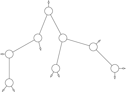

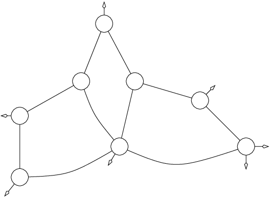
Given a binary tree , the local closure can be performed greedily until no more local closure is possible. Each local closure creates a new entire edge, maybe making a new local closure possible. It is easy to see that the final map, called the partial closure of , does not depend on the order of the local closures. Indeed, a cyclic parenthesis word is associated to the counter-clockwise boundary of the tree, with an opening parenthesis of weight 3 for a stem and a closing parenthesis for a side of entire edge; then the future local closures correspond to matchings of the parenthesis word. An example of partial closure is shown in Figure 4(c).
Complete closure
Let us now complete the partial closure operation to obtain a dissection of the hexagon with quadrangular faces. An outer entire half-edge is an half-edge belonging to an entire edge and incident to the outer face. Observe that a binary tree with nodes has stems and outer entire half-edges. Each local closure decreases by 1 the number of stems and by 2 the number of outer entire half-edges. Hence, if denotes the number of (unmatched) stems in the partial closure of , there are outer entire half-edges. Moreover, stems delimit intervals of inner half-edges on the contour of the outer face; these intervals have length at most 2, otherwise a local closure would be possible. Let be the number of such intervals of length 1 and be the number of such intervals of length 0 (that is, the number of nodes incident to two unmatched stems). Then and are clearly related by the relation .
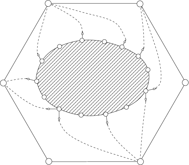

The complete closure consists in completing all unmatched stems with half-edges incident to vertices of the hexagon in the unique way (up to rotation of the hexagon) that creates only quadrangular bounded faces. Figure 5(a) illustrates the complete closure for the case , and a particular example is given in Figure 5(b).
Lemma 4.1
The closure of a binary tree is an irreducible dissection of the hexagon.
Proof.
Assume that there exists a separating 4-cycle in the closure of . Let be the number of vertices in the interior of . Then there are edges in the interior of according to Euler’s relation. Let be a vertex of that belongs to the interior of after the closure. Consider the orientation of edges of away from (only for the sake of this proof). Then nodes of have outdegree 2, except , which has outdegree 3. This orientation naturally induces an orientation of edges of the closure-dissection with the same property (except that vertices of the hexagon have outdegree 0). Hence there are at least edges in the interior of , a contradiction. ∎∎
4.2 Tri-orientations and opening
Tri-orientations
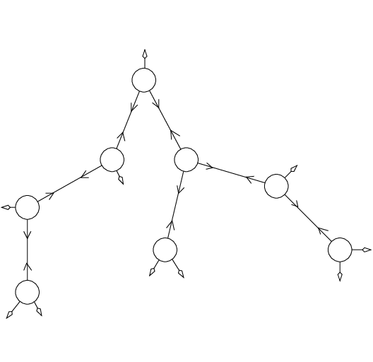
In order to define the mapping inverse to the closure, we need a better description of the structure induced on the closure map by the original tree. Let us consider orientations of the half-edges of a map (in contrast to the usual notion of orientation, where edges are oriented). An half-edge is said to be inward if it is oriented toward its origin and outward if it is oriented out of its origin. If a map is endowed with an orientation of its half-edges, the outdegree of a vertex is naturally defined as the number of its incident half-edges oriented outward. The (unique) tri-orientation of a binary tree is defined as the orientation of its half-edges such that any node has outdegree 3, see Figure 6(a) for an example. A tri-orientation of a dissection is an orientation of its inner half-edges (i.e., half-edges belonging to inner edges) such that outer and inner vertices have respectively outdegree 0 and 3, and such that two half-edges of a same inner edge can not both be oriented inward, see Figure 6(b). An edge is said to be simply oriented if its two half-edges have same direction (that is, one is oriented inward and the other one outward), and bi-oriented if they are both oriented outward.

Let be an irreducible dissection endowed with a tri-orientation. A clockwise circuit of is a simple cycle consisting of edges that are either bi-oriented or simply oriented with the interior of on their right.
Lemma 4.2
Let be an irreducible dissection with inner vertices. Then a tri-orientation of has bi-oriented edges and simply oriented edges.
If a tri-orientation of a dissection has no clockwise circuit, then its bi-oriented edges form a tree spanning the inner vertices of the dissection.
Proof.
Let and denote the numbers of simply and bi-oriented edges of . According to Euler’s relation (using the degrees of the faces), has inner edges, i.e., . Moreover, as all inner vertices have outdegree 3, . Hence and .
If the tri-orientation has no clockwise circuit, the subgraph induced by the bi-oriented edges has edges, no cycle (otherwise the cycle could be traversed clockwise, as all its edges are bi-oriented), and is incident to at most vertices, which are the inner vertices of . According to a classical result of graph theory, is a tree spanning the inner vertices of . ∎∎
Closure-tri-orientation of a dissection
Let be a dissection obtained as the closure of a binary tree . The tri-orientation of clearly induces via the closure a tri-orientation of , called closure-tri-orientation. On this tri-orientation, bi-oriented edges correspond to inner edges of the original binary tree, see Figure 6(b).
Lemma 4.3
A closure-tri-orientation has no clockwise circuit.
Proof.
Since vertices of the hexagon have outdegree 0, they can not belong to any circuit. Hence clockwise circuits may only be created during a local closure. However closure edges are simply oriented with the outer face on their right, hence may only create counterclockwise circuits. ∎∎
This property is indeed quite strong: the following theorem ensures that the property of having no clockwise circuit characterizes the closure-tri-orientation and that a tri-orientation without clockwise circuit exists for any irreducible dissection. The proof of this theorem is delayed to Section 8.
Theorem 4.4
Any irreducible dissection has a unique tri-orientation without clockwise circuit.
Recovering the tree: the opening mapping
Lemma 4.2 and the present section give all necessary elements to describe the inverse mapping of the closure, which is called the opening: let be an irreducible dissection endowed with its (unique by Theorem 4.4) tri-orientation without clockwise circuit. The opening of is the binary tree obtained from by deleting outer vertices, outer edges, and all inward half-edges.
4.3 The closure is a bijection
In this section, we show that the opening is inverse to the closure. By construction of the opening, the following lemma is straightforward:
Lemma 4.5
Let be an irreducible dissection obtained as the closure of a binary tree . Then the opening of is .
Conversely, the following also holds:
Lemma 4.6
Let be a binary tree obtained as the opening of an irreducible dissection . Then the closure of is .
Proof.
The proof relies on the definition of an order for removing inward half-edges. Start with the half-edges incident to outer vertices (that are all oriented inward): this clearly inverses the completion step of the closure. Each further removal must correspond to a local closure, that is, the removed half-edge must have the outer face on its right.
Let be the submap of the dissection induced by remaining half-edges after removals. Then covers the inner vertices, and, as long as some inward half-edge remains, it has at least entire edges (see Lemma 4.2). Hence, there is at least one cycle, and a simple one can be extracted from the boundary of the outer face of . Since there is no clockwise circuit, at least one edge of is simply oriented with the interior of on its left; the corresponding inward half-edge can be selected for the next removal. ∎∎
Theorem 4.7
For each , the closure mapping is a bijection between the set of binary trees with nodes and the set of irreducible dissections with inner vertices.
For each integer pair with , the closure mapping is a bijection between the set of bicolored binary trees with black nodes and white nodes, and the set of bicolored irreducible dissections with black inner vertices and white inner vertices.
The inverse mapping of the closure is the opening.
We can state three analogous versions of Theorem 4.7 for rooted objects:
Theorem 4.8
The closure mapping induces the following correspondences between sets of rooted objects:
Proof.
We define a bi-rooted irreducible dissection as a rooted irreducible dissection endowed with its tri-orientation without clockwise circuit and where a simply oriented edge is marked. We write for the set of bi-rooted irreducible dissections with inner vertices. Opening and rerooting on the stem corresponding to the marked edge defines a surjection from onto , for which each element of has clearly six preimages, since the dissection could have been rooted at any edge of the hexagon. Moreover, erasing the mark clearly defines a surjection from to , for which each element of has preimages according to Lemma 4.2. Hence, the closure defines a -to-6 mapping between and . The proof of the -to-3 correspondence between and is the same.
The -to-3 correspondence between and induced by the closure can be proved similarly, with the difference that the marked simply oriented edge has to have a black vertex as origin. Then the result follows from the fact that an object of endowed with its tri-orientation without clockwise circuit has simply oriented edges whose origin is a black vertex. ∎∎
Let us mention that the -to-3 correspondence between and is a key ingredient to the planar graph generators presented in [20].
The coefficient is well-known to be the -th Catalan number , and refinements of the standard proofs yield , as detailed below in Section 4.5. Theorem 4.8 thus implies the following enumerative results:
Corollary 4.9
The coefficients counting rooted irreducible dissections have the following expressions,
| (2) |
| (3) |
These enumerative results have already been obtained by \citeNMu using algebraic methods. Our method provides a direct bijective proof.
Notice that the cardinality of is where is the -th super-Catalan number of order . (These numbers are discussed by \citeNGe.) Our bijection gives an interpretation of these numbers for .
4.4 Specialization to triangulations
A nice feature of the closure mapping is that it specializes to a bijection between plane triangulations and a simple subfamily of binary trees. In this way, we get the first bijective proof for the formula giving the number of unrooted plane triangulations with vertices, found by \citeNBr, and recover the counting formula for rooted triangulations, already obtained by \citeNT62 and by \citeNPS03b using a different bijection.
Theorem 4.10
The closure mapping is a bijection between the set of (unrooted) plane triangulations with inner vertices and the set of bicolored binary trees with black nodes and no stem (i.e., leaf) incident to a black node.
The closure mapping induces the following correspondence between the set of rooted triangulations with inner vertices and the set of trees in rooted at a stem:
Proof.
Plane triangulations are exactly 3-connected planar maps where all faces have degree 3. Hence, the angular mapping with border (Theorem 3.2) induces a bijection between and the set of complete bicolored irreducible dissections with inner black vertices and all inner white vertices of degree 3. In a tri-orientation, the indegree of each inner white vertex is and the indegree of each outer white vertex is , hence the dissections considered here have no ingoing half-edge incident to a white vertex. Hence the opening of the dissection (by removing ingoing half-edges) is a binary tree with no stem incident to a black node. Conversely, starting from such a binary tree, the half-edges created during the closure mapping are opposite to a stem. As all stems are incident to white vertices, the half-edges created are incident to black vertices. Hence the degree of each white vertex does not increase during the closure mapping, i.e., remains equal to 3 for inner white vertices and equal to 2 for outer white vertices. This concludes the proof of the bijection .
The bijection follows easily (see the proof of Theorem 4.8), using the fact that a tree of has leaves. ∎ ∎


This bijection, illustrated in Figure 7, makes it possible to count plane unrooted and rooted triangulations, as the subfamily of binary trees involved is easily enumerated.
Corollary 4.11
For , the number of rooted triangulations with inner vertices is
The number of unrooted plane triangulations with inner vertices is
Proof.
Let be the class of rooted binary trees with no leaf incident to a black node and let be the class of rooted binary trees where the root leaf is incident to a black node and all other leaves are incident to white nodes. Let and be the generating functions of and with respect to the number of black nodes. Clearly the two subtrees pending from the (white) root node of a tree of are either empty or in . Hence . Similarly, a tree in decomposes at the root node into two trees in , so that . Hence, is equal to the generating function of quaternary trees, and is equal to the generating function of pairs of quaternary trees (the empty tree being allowed). Using a Lukaciewicz encoding and the cyclic lemma, the number of pairs of quaternary trees with a total of nodes is easily shown to be . This expression of and the -to-3 correspondence between and yield the expression of .
Let us now prove the formula for . Clearly, the only possible symmetry for a bicolored binary tree is a rotation of order 3. Let be the set of trees of with a rotation symmetry and let be the set of trees of with no symmetry. Let and be the sets of trees of and that are rooted at a leaf. It is easily shown that a tree of has leaves. Clearly the tree gives rise to rooted trees if it is asymmetric and gives rise to rooted trees if it is symmetric. Hence and . Using and , we obtain
The centre of rotation of a tree in is either a black node, in which case for some integer , or is a white node, in which case for some integer . In the first case, a tree is obtained by attaching to a black node 3 copies of a tree in . Hence . In the second case, a tree is obtained by attaching to a white node 3 copies of a tree in . Hence . The result follows. ∎ ∎
4.5 Counting, coding and sampling rooted bicolored binary trees


4.5.1 From a bicolored tree to a pair of words
There exist general methods to encode a family of trees specified by several parameters. This section makes such methods explicit for the family of bicolored binary trees. Let be a black-rooted bicolored binary tree with black nodes and white nodes. Doing a depth-first traversal of from left to right, we obtain a word of length on the alphabet represented in Figure 8(a), see Figure 9 for an example, the mapping being denoted by . Classically, the sum of the weights of the letters of any strict prefix of is nonnegative and the sum of the weights of the letters of is equal to -1. In addition, is the unique word in its cyclic equivalence-class that has these two properties.
The second step is to map to a pair of words such that: {longitem}
is a word of length on the alphabet shown in Figure 8(b) with black-node-letters.
is a word of length on the alphabet shown in Figure 8(c) with white-node-letters. Figure 9 illustrates the mapping on an example.
4.5.2 Inverse mapping: from a pair of words to a tree
Conversely, let be a pair of words such that is of length on and has black-node-letters, and is of length on and has white-node-letters. First, to the pair we associate a word of length on by doing the inverse of the mapping shown in the right part of Figure 9. The word has the property that the sum of the weights of its letters is equal to -1. There is a unique word in the cyclic equivalence-class of such that the sum of the weights of the letters of any strict prefix is nonnegative. We associate to the binary tree of obtained by doing the inverse of the mapping shown in Figure 9.
This method allows us to sample uniformly objects of in linear time and ensures that
| (4) |
5 Application: counting rooted 3-connected maps
5.1 Generating functions of rooted dissections
Even if the counting formulas obtained in Corollary 4.9 are simple, it proves useful to have an expression of the corresponding generating functions. Indeed, the decomposition-method we develop is suitably handled by generating functions.
Let and be the series of black-rooted and white-rooted bicolored binary trees. By decomposition at the root, and are the solutions of the system:
| (5) |
Define an edge-marked bicolored binary tree as a bicolored binary tree with a marked inner edge. Let be the set of edge-marked bicolored binary trees with black nodes and white nodes. Cutting the marked edge of such a tree yields a pair made of a black-rooted and a white-rooted binary tree. As a consequence, the generating function counting edge-marked bicolored binary trees is , i.e., .
Let us consider bi-rooted objects as in the proof of Theorem 4.8; since any object of has white leaves (connected to a black node) and black leaves (connected to a white node),
Similarly, counting in two ways the objects of having a marked edge yields
Thus, we have (using (3)), so that
| (6) |
Substituting and by , we obtain:
| (7) |
where is the generating function of binary trees according to the number of inner nodes.
5.2 Generating function of rooted 3-connected maps
Injection from to
Let us consider the mapping defined on rooted quadrangulations by the removal of the root-edge and rerooting on the next edge in counterclockwise order around the root-vertex; is clearly injective, and for any quadrangulation , has only quadrangular faces but the outer one, which is hexagonal. In addition, can not have more separating 4-cycles than . Hence the restriction of to is an injection from to , more precisely from to and from to .
It is however not a bijection, since the inverse edge-adding operation , performed on an irreducible dissection, can create a separating 4-cycle on the obtained quadrangulation. Precisely, given a rooted irreducible dissection —with the root-vertex and the vertex of the hexagon opposite to — a path of length 3 between and is called a decomposition path. The two paths of edges of the hexagon connecting to are called outer decomposition paths, and the other ones, if any, are called inner decomposition paths of .
Observe that inner decomposition paths of are in one-to-one correspondence with separating 4-cycles of the quadrangulation (i.e., the quadrangulation obtained from by adding a root-edge between and oriented out of ).
A rooted irreducible dissection without inner decomposition path is said to be undecomposable. The corresponding class is denoted by . The discussion on decomposition paths yields the following result.
Lemma 5.1
Denote by the set of rooted undecomposable dissections with inner vertices and by the set of rooted undecomposable dissections with inner black vertices and inner white vertices. Then is in bijection with and is in bijection with .
Proof.
A rooted irreducible quadrangulation is mapped by to a rooted dissection such that the inverse edge-adding operation does not create a separating 4-cycle, i.e., an undecomposable dissection. Moreover, Euler’s relation ensures that the image of a quadrangulation with faces has inner vertices. By injectivity, is bijective to its image, i.e., is a bijection between and ; and a bijection between and . The result follows, as and are respectively in bijection with and via the angular mapping (Theorem 3.1). ∎ ∎
Thanks to Lemma 5.1, enumerating rooted 3-connected maps reduces to enumerating rooted undecomposable dissections.
Decomposition of rooted irreducible dissections
Since irreducible dissections do not have multiple edges nor cycles of odd length, decomposition paths satisfy the following properties:
Lemma 5.2
Let be a rooted irreducible dissection, and let and be two different decomposition paths of . Then: {longitem}
either , in which case and are said to be internally disjoint;
or there exists one inner vertex such that , in which case and are said to be upper or lower joint whether is adjacent to or .
Lemma 5.2 implies in particular that two decomposition paths can not cross each other. Hence the decomposition paths of an irreducible dissection follow a left-to-right order, from the outer decomposition path containing the root —called left outer path— to the other outer decomposition path —called right outer path.
Lemma 5.3
Let be a rooted irreducible dissection, and let and be two upper joint (resp. lower joint) decomposition paths of . Then the interior of the area delimited by and consists of a unique face incident to (resp. to ).
Proof.
Follows from the fact that the interior of each 4-cycle of is a face. ∎ ∎
Decomposition word of an irreducible dissection
Let and let be the sequence of decomposition paths of ordered from left to right. Let us consider the alphabet ; the decomposition word of is the word of length on such that, for any : if and are upper joint, then ; if and are lower joint, then ; if and are internally disjoint, then , where is the undecomposable dissection delimited by and , rooted at the first edge of and with as root-vertex, see Figure 10. This encoding is injective, an easy consequence of Lemma 5.3.
-5,-4)(24,4)
Characterization of decomposition words of elements of
The fact that has no separating 4-cycle easily implies that its decomposition word has no factor nor , and these are the only forbidden factors. Moreover, as a dissection has at least one inner vertex, a decomposition word can neither be the empty word, nor the one-letter words and , nor the two-letter words and . It is easily seen that all other words encode irreducible dissections of the hexagon.
This leads to the following equation linking the generating functions and counting and according to the number of inner vertices,
| (8) |
Similarly, let and . Then the characterization of the coding words gives
| (9) |
Theorem 5.4
Let be the number of rooted 3-connected maps with edges and the number of rooted 3-connected maps with vertices and faces. Then
where , and
| (10) |
where .
6 Application: sampling rooted 3-connected maps
6.1 Sampling rooted 3-connected maps with edges
Theorem 4.8 (first identity) ensures that the following algorithm samples rooted 3-connected maps with edges uniformly at random:
- 1.
Sample an object uniformly (e.g. using parenthesis words).
- 2.
Perform the closure of to obtain an irreducible dissection with vertices. Choose randomly one of the six edges of the hexagon of to carry the root. If is not undecomposable, then reject and restart.
- 3.
Connect by a new edge the root-vertex of to the opposite outer vertex. Take as root edge, with the same root-vertex as in . This gives a rooted irreducible quadrangulation with faces.
- 4.
Return the rooted 3-connected map in associated to by the angular mapping.
Proposition 6.1
The success probability of the sampler at each trial is equal to , which satisfies
Hence, the number of rejections follows a geometric law whose mean is asymptotically . As the closure mapping has linear-time complexity, the sampling algorithm has expected linear-time complexity.
6.2 Sampling rooted 3-connected maps with vertices and faces
Similarly, Theorem 4.8 (third identity), ensures that the following algorithm samples rooted 3-connected maps with vertices and faces uniformly at random:
- 1.
Sample an object uniformly at random. A simple method is described in Section 4.5.2.
- 2.
Perform the closure of to obtain an irreducible dissection with inner black vertices and inner white vertices. Choose randomly the root-vertex among the three black vertices of the hexagon. If the dissection is not undecomposable, then reject and restart.
- 3.
Connect by a new edge the root-vertex of to the opposite outer vertex. Take as root edge, with the same root-vertex as in . This gives a rooted irreducible quadrangulation with black vertices and white vertices.
- 4.
Return the rooted 3-connected map in associated to by the angular mapping.
Proposition 6.2
The success probability of the sampler at each trial is equal to . Let ; if and are correlated by as , then
Hence, when , the number of rejections follows a geometric law whose mean is asymptotically . Under these conditions, the sampling algorithm has an expected linear-time complexity, the linearity factor being asymptotically proportional to .
Moreover, in the worst case of triangulations where , the mean number of rejections is quadratic, so that the sampling complexity is cubic.
7 Application: coding 3-connected maps
This section introduces an algorithm, derived from the inverse of the closure mapping, to encode a 3-connected map. Precisely, the algorithm encodes an outer-triangular 3-connected map, but it is then easily extended to encode any 3-connected map. Indeed, if the outer face of is not triangular, fix three consecutive vertices , and incident to the outer face of and link and by an edge to obtain an outer-triangular 3-connected planar map ; the coding of is obtained as the coding of plus one bit indicating if an edge-addition has been done.
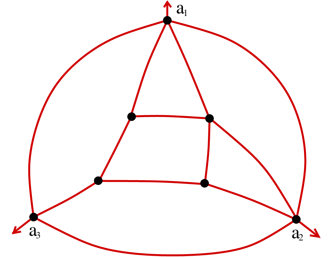
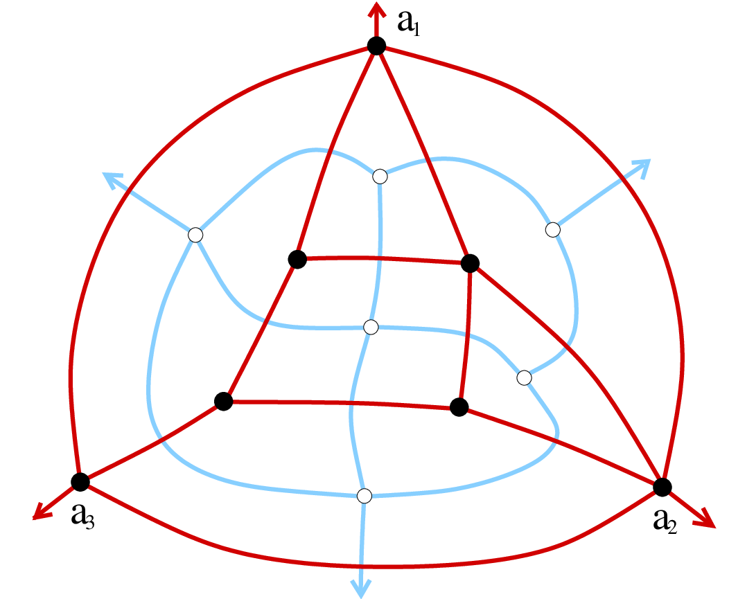
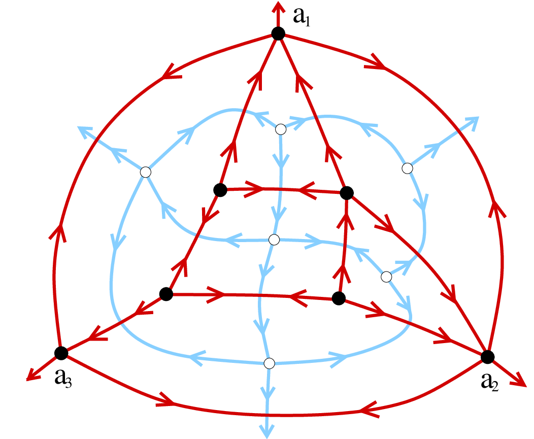

7.1 Description of the coding algorithm
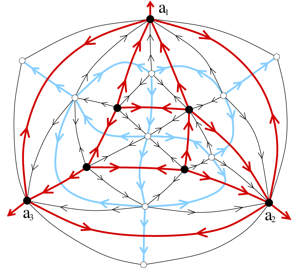
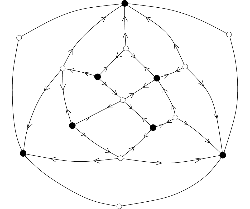
Let be an outer-triangular 3-connected map and let be its derived map, as defined in Section 3.2. The coding algorithm relies on the following steps, illustrated in Figure 11.
7.1.1 Compute a particular orientation of the derived map (Fig. 11(b)-(c))
The first step of the algorithm is to compute a specific orientation of the edges of the derived map , such that has no clockwise circuit, each primal or dual vertex has outdegree 3 and each edge-vertex has outdegree 1. Such an orientation of exists and is unique, as we will see in Theorem 8.1. A linear time algorithm to compute is given in Section 9.
7.1.2 Compute the irreducible dissection associated to (Fig. 11(d))
Consider the bicolored complete irreducible dissection associated to by the bijection presented in Section 3.2 (and reformulated in Section 3.3), i.e., the dissection having the same derived map as . Notice that has inner faces if has edges. Hence, according to Euler’s relation, has inner vertices. Similarly, if has vertices and inner faces, then has black vertices and white vertices.
7.1.3 Compute the tri-orientation of without clockwise circuit (Fig. 11(d))
We orient each half-edge of belonging to an inner edge as follows: is directed inward if its incident vertex belongs to the hexagon; otherwise, receives the orientation of the cw-following edge of . As shown in Section 8 (more precisely in Lemma 8.13, composed with the correspondence of Figure 13), this process yields the unique tri-orientation of without clockwise circuit.
7.1.4 Open the dissection into a binary tree (Fig. 11(f))
Once the tri-orientation without clockwise circuit is computed, is opened into a binary tree , by deleting outer vertices, outer edges, and all ingoing half-edges (see Section 4.2).
7.1.5 Encode the tree
First, choose an arbitrary leaf of , root at this leaf, and encode the obtained rooted binary tree using a parenthesis word (also called Dyck word). The opening of a 3-connected map with edges is a binary tree with inner nodes, yielding an encoding Dyck word of length .
Similarly, the opening of a 3-connected map with vertices and inner faces is a black-rooted bicolored binary tree with black nodes and white nodes. A black-rooted bicolored binary trees with a given number of black and white nodes is encoded by a pair of words, as explained in Section 4.5.1. Then the two words can be asymptotically optimally encoded in linear time, according to [7, Lem.7].
Theorem 7.1
The coding algorithm has linear-time complexity and is asymptotically optimal: the number of bits per edge of the code of a map in (resp. in ) is asymptotically equal to the binary entropy per edge, defined as (resp. ).
Proof.
It is clear that the encoding algorithm has linear-time complexity, provided the algorithm computing the constrained orientation without clockwise circuit of the derived map has linear-time complexity (which will be proved in Section 9 and Section 10).
According to Corollary 4.9, Proposition 6.1 and 6.2, and are bounded by fixed polynomials. Hence, the entropy per edge of and are asymptotically equal, and the binary entropy per edge of and are asymptotically equal. As the encoding of objects of () using parenthesis words is asymptotically optimal, the encoding of objects of (, respectively) is also asymptotically optimal. ∎∎
8 Proof of Theorem 4.4
This section is devoted to the proof of Theorem 4.4, which states that each irreducible dissection has a unique tri-orientation without clockwise circuit.
8.1 -orientations and outline of the proof
Definition
Let be a planar map. Consider a function . An -orientation of is an orientation of the edges of such that the outdegree of each vertex of is . If an -orientation exists, then the function is said to be feasible for .
Existence and uniqueness of -orientations
Theorem 8.1 (([17]))
Given a planar map and a feasible function , there exists a unique -orientation of without clockwise circuit. This -orientation is called the minimal 11 1 The term minimal refers to the fact that the set of all -orientations of forms a distributive lattice, the “flip” operation being a circuit reversion. -orientation of .
Given the derived map of an outer-triangular 3-connected planar map, the function such that for all primal and dual vertices and for all edge-vertices is a feasible function.
Theorem 8.1 ensures uniqueness of the orientation without clockwise circuit of a graph with prescribed outdegree for each vertex. However, this property does not directly imply uniqueness in Theorem 4.4, because a tri-orientation has bi-oriented edges.
To use Theorem 8.1, we work with the derived map of an irreducible dissection , as defined in Section 3.3. We have defined derived maps only for a subset of irreducible dissections, namely for bicolored complete irreducible dissections (recall that these are bicolored dissections such that the 3 outer white vertices have degree 2). As a consequence, a first step toward proving Theorem 4.4 is to reduce its proof to the proof of existence and uniqueness of a so-called complete-tri-orientation (a slight adaptation of the definition of tri-orientation) without clockwise circuit for any bicolored complete irreducible dissection.
We prove that a complete-tri-orientation without clockwise circuit of a bicolored complete irreducible dissection is transposed injectively into an -orientation without clockwise circuit of its derived map . By injectivity and by uniqueness of the -orientation without clockwise circuit of , this implies uniqueness of a tri-orientation without clockwise circuit for .
The final step will be to prove that an -orientation without clockwise circuit of is transposed into a complete-tri-orientation without clockwise circuit of . By existence of an -orientation without clockwise circuit for (Theorem 8.1), this implies the existence of a complete-tri-orientation without clockwise circuit of .
8.2 Reduction to the case of bicolored complete dissections
Introduction
The aim of this section is to reduce the proof of Theorem 4.4 to the class of complete bicolored irreducible dissections. We state the following proposition where the term “complete-tri-orientation”, to be defined later, is a slight adaptation of the notion of tri-orientation.
Proposition 8.2
The existence and uniqueness of a complete-tri-orientation without clockwise circuit for any bicolored complete irreducible dissection implies the existence and uniqueness of a tri-orientation without clockwise circuit for any irreducible dissection, i.e., implies Theorem 4.4.
The rest of this subsection is devoted to the proof of Proposition 8.2. The proof is done in two steps. First, reduce the proof of Theorem 4.4 to the existence and uniqueness of a tri-orientation without clockwise circuit for any bicolored complete irreducible dissection. Then, prove that this reduces to the existence and uniqueness of a complete-tri-orientation without clockwise circuit for any bicolored complete irreducible dissection.
Completion of a bicolored irreducible dissection
For any bicolored irreducible dissection , we define its completed dissection as follows . For each white vertex of the hexagon, we denote by () the outer edge starting from with the interior of the hexagon on the left (right, respectively) and denote by and the neighbours of incident to and to . We perform the following operation: if has degree at least 3, a new white vertex is created outside of the hexagon and is linked to and to by two new edges and , see Figure 12. The vertex is said to cover the vertex .
The dissection obtained is a bicolored dissection of the hexagon such that the three white vertices of the hexagon have two incident edges, see the transition between Figure 13(a) and Figure 13(b) (ignore here the orientation of edges).
Lemma 8.3
The completion of a bicolored irreducible dissection is a bicolored complete irreducible dissection.
Proof.
The outer white vertices of have degree 2 by construction. Hence, we just have to prove that is irreducible. As is irreducible, if a separating 4-cycle appears in when the completion is performed, then it must contain a white vertex of the hexagon of added during the completion, so as to cover an outer white vertex of degree greater than 2. Two edges of are the edges and incident to in . The two other edges and of form a path of length 2 connecting the vertices and and passing by the interior of (otherwise, would enclose a face). As is irreducible, the 4-cycle of consisting of the edges , , and delimits a face. Hence and are incident to the same inner face of , which implies that has degree 2, a contradiction. ∎∎
Tri-orientations
Let be a bicolored irreducible dissection and let be its completed bicolored dissection. We define a mapping from the tri-orientations of to the tri-orientations of . Given a tri-orientation of , we remove the edges that have been added to obtain from , erase the orientation of the edges of the hexagon of , and orient inward all inner half-edges incident to an outer vertex of . We obtain thus a tri-orientation of , see the transition between Figure 13(b) and Figure 13(a).
Lemma 8.4
Let be a tri-orientation of without clockwise circuit. Then the tri-orientation of has no clockwise circuit.
For each tri-orientation of without clockwise circuit, there exists a tri-orientation of without clockwise circuit such that .
Proof.
The first point is trivial, as the tri-orientation is just obtained by removing some edges and some orientations of half-edges.
For the second point, the preimage is constructed as follows. Consider each white vertex of the hexagon of which has degree at least 3. Let ( be the series of half-edges incident to in in counter-clockwise order around , with and belonging respectively to the edges and . As , the vertex gives rise to a covering vertex with two incident edges and such that the edges , , and form a new face . The edges and become inner edges of when is added, and have thus to be directed.
We orient the two half-edges of and respectively toward and toward , see Figure 12. The vertex receives thus two outgoing half-edges, and we have to give to a third outgoing half-edge. The suitable choice to avoid the appearance of a clockwise circuit is to orient outward, see Figure 12. Indeed, assume a contrario that a simple clockwise circuit is created. Then the circuit must pass by . It goes into using one of the half-edges directed toward , i.e., . Moreover, it must go out of using the half-edge (indeed, if the circuit uses or to go out of , then it reaches an outer vertex, which has outdegree 0). Hence, the interior of the clockwise circuit must contain all faces incident to that are on the right of when we traverse from and go out using . Hence, the interior of must contain the new face of , see Figure 12. But is incident to outer edges of , hence the clockwise circuit must pass by outer edges of , which are not oriented, a contradiction. Thus, we have constructed a tri-orientation of without clockwise circuit and such that . An example of this construction can be seen as the transition between Figure 13(a) and Figure 13(b). ∎ ∎


Lemma 8.5
The existence and uniqueness of a tri-orientation without clockwise circuit for any bicolored complete irreducible dissection implies the existence and uniqueness of a tri-orientation without clockwise circuit for any irreducible dissection, i.e., implies Theorem 4.4.
Complete-tri-orientations
A complete-tri-orientation of a bicolored complete irreducible dissection is an orientation of the half-edges of that satisfies the following conditions (very similar to the conditions of a tri-orientation): all black vertices and all inner white vertices of have outdegree 3, the three white vertices of the hexagon have outdegree 0, and the two half-edges of an edge of can not both be oriented inward. The difference with the definition of tri-orientation is that the half-edges of the hexagon are oriented, with prescribed outdegree for the outer vertices. Similarly as in a tri-orientation, edges of are distinguished into simply-oriented edges and bi-oriented edges.
Lemma 8.6
Let be a bicolored complete irreducible dissection endowed with a complete-tri-orientation without clockwise circuit. Then the subgraph of consisting of the bi-oriented edges of is a tree incident to all vertices of except the three outer white vertices.
Proof.
We reason similarly as in Lemma 4.2. Let and be the numbers of bi-oriented and simply oriented edges of . From Euler’s relation (using the degrees of the faces of ), has edges, i.e., . In addition, the inner vertices and the three black (resp. white) vertices of the hexagon of have outdegree 3 (resp. 0). Hence, . Thus, and . Hence, the subgraph has edges, has no cycle (otherwise, a clockwise circuit of would exist), and is incident to at most vertices, which are the inner vertices and the three outer black vertices of . A classical result of graph theory ensures that is a tree spanning these vertices. ∎ ∎
Lemma 8.7
Let be a bicolored complete irreducible dissection endowed with a complete-tri-orientation without clockwise circuit. Then, for each outer black vertex of , the unique outgoing inner half-edge incident to belongs to a bi-oriented edge.
Proof.
The subgraph consisting of the bi-oriented edges of is a tree spanning all vertices of except the three outer white vertices. Hence, there is a bi-oriented edge incident to each black vertex of the hexagon and this edge consitutes the third outgoing edge of . ∎ ∎
Let be a bicolored complete irreducible dissection and be a complete-tri-orientation of without clockwise circuit. We associate to a tri-orientation as follows: erase the orientation of the edges of the hexagon of ; for each black vertex of the hexagon, change the orientation of the unique outgoing inner half-edge of . According to Lemma 8.7, belongs to a bi-oriented edge , so that the change of orientation of turns into an edge simply oriented toward . Thus, the obtained orientation is a tri-orientation.
Lemma 8.8
Let be a bicolored complete irreducible dissection. Let be a complete-tri-orientation of without clockwise circuit. Then the tri-orientation of has no clockwise circuit.
For each tri-orientation of without clockwise circuit, there exists a complete-tri-orientation of without clockwise circuit such that .
Proof.
The first point is trivial. For the second point, we reason similarly as in Lemma 8.4. For each black vertex of the hexagon of , let ( be the sequence of half-edges of incident to in counter-clockwise order around , with and belonging to the two outer edges and of that are incident to . To construct the preimage of , we make the edges and simply oriented toward their incident white vertex. The third outgoing half-edge is chosen to be , which is the “leftmost” inner half-edge of . An argument similar as in the proof of the second point of Lemma 8.4 ensures that this choice is judicious to avoid the creation of a clockwise circuit. An example of this construction is shown in Figure 13(b)-(c). ∎ ∎
8.3 Transposition rules for orientations
Let be a bicolored complete irreducible dissection and let be the derived map of . We associate to a complete-tri-orientation of an orientation of the edges of of as follows, see Figure 14: each edge —with the primal/dual vertex and the edge-vertex— receives the direction of the half-edge of following in ccw order around .


Lemma 8.9
Let be a bicolored complete irreducible dissection endowed with a complete-tri-orientation without clockwise circuit. Then the orientation of the derived map of obtained using the transposition rules has the following properties:
- •
each primal or dual vertex of has outdegree 3.
- •
each edge-vertex of has outdegree 1.
In other words, the orientation of obtained by applying the transposition rules is an -orientation.
Proof.
The first point is trivial. For the second point, let be an inner face of and the associated edge-vertex of (we recall that is the intersection of the two diagonals of ). The transposition rules for orientation ensures that the outdegree of in is the number of inward half-edges of incident to . Hence, to prove that each edge-vertex of has outdegree 1, we have to prove that for each inner face of . Observe that is a positive number, otherwise the contour of would be a clockwise circuit. Let be the number of inner vertices of . Euler’s relation implies that has inner faces and half-edges. By definition of a complete-tri-orientation, half-edges are outgoing. Hence, half-edges are ingoing. Among these ingoing half-edges, exactly three are incident to the outer face (see Figure 13(c)). Hence, has half-edges incident to an inner face, so that . As is a sum of positive numbers adding to , the pigeonhole’s principle ensures that for each inner face of . ∎ ∎
8.4 Uniqueness of a tri-orientation without clockwise circuit
The following lemma is the companion of Lemma 8.9 and is crucial to establish the uniqueness of a tri-orientation without clockwise circuit for any irreducible dissection.
Lemma 8.10
Let be a bicolored complete irreducible dissection endowed with a complete-tri-orientation without clockwise circuit. Let be the derived map of . Then the -orientation of obtained from by the transposition rules has no clockwise circuit.
Proof.
Assume that has a clockwise circuit . Each edge of connects an edge-vertex and a vertex of the original dissection . Hence, the circuit consists of a sequence of pairs of consecutive edges of such that goes from a vertex of the dissection toward an edge-vertex of and goes from toward a vertex of the dissection. Let be the sequence of edges of between and in clockwise order around , so that ; and and let be their respective extremities, so that and . Notice that .
As each edge-vertex has outdegree 1 in and as is going out of , the edges are directed toward . Hence, the transposition rules for orientations ensure that the edges , for , are all bi-oriented or oriented from to in the complete-tri-orientation of . Hence, we can go from to passing by the exterior of and using only edges of , see Figure 15 for an example, where .
Concatenating the paths of edges of associated to each pair of , we obtain a closed oriented path of edges of enclosing the interior of on its right. Clearly, a simple clockwise circuit can be extracted from this closed path, see Figure 16. As the complete-tri-orientation has no clockwise circuit, this yields a contradiction. ∎ ∎
Proposition 8.11
Each irreducible dissection has at most one tri-orientation without clockwise circuit.
Proof.
Let be a bicolored complete irreducible dissection and its derived map. A first important remark is that the transposition rules for orientations clearly define an injective mapping. In addition, Lemma 8.10 ensures that the image of a complete-tri-orientation of without clockwise circuit is an -orientation of without clockwise circuit. Hence, injectivity of the mapping and uniqueness of an -orientation without clockwise circuit of (Theorem 8.1) ensure that has at most one complete-tri-orientation without clockwise circuit. Hence, Proposition 8.2 implies that each irreducible dissection has at most one tri-orientation without clockwise circuit. ∎ ∎
8.5 Existence of a tri-orientation without clockwise circuit
Inverse of the transposition rules
Let be a bicolored complete irreducible dissection and its derived map. Given an -orientation of , we associate to this orientation an orientation of the half-edges of by performing the inverse of the transposition rules: each half-edge of receives the orientation of the edge of that follows in clockwise order around its incident vertex, see Figure 14(b).
Lemma 8.12
Let be an irreducible dissection and the derived map of , endowed with its minimal -orientation. Then the inverse of the transposition rules for orientations yields a complete-tri-orientation of .
Proof.
The inverse of the transposition rules is clearly such that a vertex has the same outdegree in the orientation of as in the -orientation of . Hence, each vertex of has outdegree 3 except the 3 outer white vertices that have outdegree 0, see Figure 14(b).
To prove that the orientation of is a complete-tri-orientation, it remains to show that the two half-edges of an edge of can not both be oriented inward. Assume a contrario that there exists such an edge . The transposition rules for orientation and the fact that each edge-vertex of has outdegree 1 imply that the boundary of the face of associated to is a clockwise circuit, see Figure 17. This yields a contradiction with the minimality of the -orientation. ∎ ∎
Lemma 8.13
Let be a bicolored complete irreducible dissection and let be its derived map. Then the complete-tri-orientation of associated with the minimal -orientation of has no cw circuit.
Proof.
Let be the minimal -orientation of and let be the associated complete-tri-orientation of . Assume that has a clockwise circuit . For each vertex on , we denote by the half-edge of starting from with the interior of on its right, and we denote by the edge of that follows in clockwise order around . As is a clockwise circuit for , is going out of . Hence, by definition of the transposition rules, is going out of . Observe that, in the interior of , is the most counter-clockwise edge of incident to .
We use this observation to build iteratively a clockwise circuit of , yielding a contradiction. First we state the following result proved in [17]: “for each vertex there exists a simple oriented path in , called the straight path of , which starts at and ends at a vertex incident to the outer face of ". Let be a vertex on , and be the straight path starting at for the orientation . Then has to reach at a vertex different from . Denote by the part of between and , by the part of the clockwise circuit between and , and by the cycle enclosed by the concatenation of and . Let be the straight path starting at . The fact that is the most counterclockwise incident edge of in the interior of ensures that starts in the interior of . Then, the path has to reach at a vertex . We denote by the part of the path between and . If belongs to , then the concatenation of the part of between and and of the part of between and is a clockwise circuit, a contradiction. Hence, is on strictly between and . We denote by the concatenation of and , and by the part of going from to . As is strictly between and , is strictly included in . Finally, we denote by the cycle made of the concatenation of and . Hence, similarly as for the path , the straight path starting at must start in the interior of .
Then we continue iteratively, see Figure 18. At each step , we consider the straight path starting at . This path starts in the interior of the cycle , and reaches at another vertex . This vertex can not belong to , otherwise a clockwise circuit of would be created. Hence, is on strictly between and . In particular the path going from to on , is strictly included in the path going from to on , i.e., shrinks strictly at each step. Thus, there must be a step when reaches at a vertex on , creating a clockwise circuit of , a contradiction. ∎ ∎
Proposition 8.14
For each irreducible dissection, there exists a tri-orientation without clockwise circuit.
Proof.
Lemma 8.13 ensures that each bicolored complete irreducible dissection has a complete-tri-orientation without clockwise circuit; and Proposition 8.2 ensures that the existence of a complete-tri-orientation without clockwise circuit for any bicolored complete irreducible dissection implies the existence of a tri-orientation without clockwise circuit for any irreducible dissection. ∎ ∎
9 Computing the minimal -orientation of a derived map
We describe in this section a linear-time algorithm to compute the minimal -orientation of the derived map of an outer-triangular 3-connected plane graph. This result is crucial for the encoding algorithm of Section 7 to have linear time complexity (see the transition between Figure 11(b) and Figure 11(c)).
As discussed in [17], given a 3-connected map and its derived map , an -orientations of corresponds to a so-called Schnyder wood of . These Schnyder woods of 3-connected maps are the right generalisations of Schnyder woods of triangulations [39]. Quite naturally, our algorithm is a generalization of the algorithm to compute the minimal Schnyder wood of a triangulation [9]. The ideas for the extension to 3-connected maps have already been introduced by [25] and [3]. The algorithm of [3] outputs a Schnyder wood of a 3-connected map; which can be subsequently made minimal by iterated circuit reversions with a linear overall complexity, as easily follows from ideas presented in [27]. Our algorithm relies on similar principles, suitably modified so as to ouput directly the minimal Schnyder wood (i.e., the Schnyder wood associated with the minimal -orientation), also in linear time. In itself our algorithm for 3-connected maps is only slightly more involved than the algorithm for triangulations, as opposed to the correctness proof, which is much harder (see the discussion at the beginning of Section 10). Because of this we give a rather proof-oriented description of the algorithm.
Our algorithm is also of independent interest in connection with Schnyder woods, and it has applications in the context of graph drawing. Indeed, the minimal Schnyder wood orientation is also a key ingredient for the straight-line drawing algorithm presented in [6]. This algorithm relies on operations of edge-deletion, embedding of the obtained graph, and then embedding of the deleted edges. The grid size is guaranteed to be bounded by —equalling at least Schnyder’s algorithm [39]— provided the Schnyder wood used is the one associated to the minimal -orientation. An implementation of this drawing algorithm including our orientation algorithm has been made available by Bonichon in [19].
9.1 Principle of the algorithm
Let be an outer-triangular 3-connected planar graph and let be its derived map and its dual map. We denote by , and the outer vertices of in clockwise order. We describe here a linear-time iterative algorithm to compute the minimal -orientation of . The idea is to maintain a simple cycle of edges of ; at each step , the cycle, denoted by , is shrinked by choosing a so-called eligible vertex on , and by removing from the interior of all faces incident to . The eligible vertex is always different from and , so that the edge , called base-edge, is always on . The edges of ceasing to be on or in the interior of are oriented so that the following invariants remain satisfied.
Orientation invariants: {longitem}
For each edge of outside , the 4 edges of incident to the edge-vertex associated to have been oriented at a step and has outdegree 1.
All other edges of are not yet oriented. Moreover, the edges that correspond to half-edges of also receive a label in , so that the following invariants for labels remain satisfied:
Labelling invariants: {longitem}
At each step , every vertex of outside of has one outgoing half-edge for each label 1, 2 and 3 and these outgoing edges appear in clockwise order around . In addition, all edges between the outgoing edges with labels and are incoming with label , see Figure 19(a).
Let be a vertex of on having at least one incident edge of outside of . Then exactly one of these edges, denoted by , is going out of . In addition it has label 1. The edges of incident to and between and its left neighbour on are incoming with label 2; and the edges incident to in between and its right neighbour on are incoming with label 3, see Figure 19(b).
For each edge of outside of , let be the unique outgoing edge of its associated edge-vertex . Two cases can occur: {longitem}
If is an half-edge of then the two edges of incident to and forming the edge are identically labelled. This corresponds to the case where is “simply oriented”.
If is an half-edge of , we denote by the label of the edge of following in clockwise order around . Then the edge of following in counter-clockwise order around is labelled , see Figure 19(c). This corresponds to the case where is “bi-oriented”.
Actually, the labels are not needed to compute the orientation, but they will be very useful to prove that the algorithm outputs the minimal -orientation. These labels are in fact the ones of the Schnyder woods of , as discussed in [17].
In the following, we write for the submap of obtained by removing all vertices and edges outside of (at step ). In addition, we order the vertices of from left to right according to the order induced by the path , with as left extremity and as right extremity. In other words, a vertex is on the left of a vertex if the path of going from to without passing by the edge has the interior of on its right.


9.2 Description of the main iteration
Let us now describe the -th step of the algorithm, during which the cycle is shrinked so that the invariants for orientation and labelling remain satisfied. The description requires some definitions.
Definitions
A vertex of is said to be active if it is incident to at least one edge of . Otherwise, the vertex is passive. By convention, before the first step of the algorithm, the vertex is considered as active and its incident half-edge directed toward the outer face is labelled 1.
For each pair of vertices of —with is on the left of —, the path on going from to without passing by the edge is denoted by . We also write for deprived from the endvertices and .
A pair of vertices of is separating if there exists an inner face of such that and are incident to but the edges of are not all incident to . Such a face is called a separating face and the triple is called a separator. The (closed) area delimited by the path and by the path of edges of going from to with the interior of on its right is called the separated area of and is denoted by .
A vertex on is said to be blocked if it belongs to a separating pair. It is easily checked that a vertex is blocked iff it is incident to a separating face of . In particular, a non blocked vertex does not belong to any separating pair of vertices. By convention, the vertices and are always considered as blocked. A vertex on is eligible if it is active and not blocked.
Finally, for each vertex of , we define its left-connection vertex as the leftmost vertex on such that the vertices of all have degree 2 in . The path is called the left-chain of and the first edge of is called the left-connection edge of . Similarly, we define the right-connection vertex, the right-chain, and the right-connection edge of . Notice that all vertices of and of are active, as each vertex of a 3-connected graph has degree at least 3.
Operations at step
First, we choose the rightmost eligible vertex of and we call this vertex. (We will prove in Lemma 9.2 that there always exists an eligible vertex on as long as is not reduced to the edge .) Notice that this eligible vertex can not be nor because and are blocked.
We denote by the bounded faces of incident to from right to left, and by the edges of incident to from right to left. Hence, for each , corresponds to the sector between and .
An important remark is that the right-chain of is reduced to one edge. Indeed, if there exists a vertex in , then is active, as discussed above. In addition, is incident to only one inner face of , namely . As is incident to and as is non blocked, is not separating. Hence is not blocked. Thus is eligible and is on the right of , in contradiction with the fact that is the rightmost eligible vertex on .
We label and orient the edges of incident to the edge-vertices on the left-chain of and on the edges , see Figure 20:
Inner edges: For each edge with , we denote by the corresponding edge-vertex of . Orient the two edges of forming toward and give label 1 to these two edges. Orient the two other incident edges of toward , so that has outdegree 1.
Left-chain: For each edge of the left-chain of —traversed from to — different from the left-connection edge, bi-orient and give label 3 (resp. label 2) to the first (resp. second) traversed half-edge. Choose the unique outgoing edge of the edge-vertex associated to to be the edge going out of toward the interior of
Left-connection edge: If is passive, bi-orient the left-connection edge of , give label 1 to the half-edge incident to and label 3 to the other half-edge, and choose the unique outgoing edge of the edge-vertex to be the edge going out of toward the exterior of . If is active, label 3 and orient toward the two edges of forming , and orient the two dual edges incident to toward .
Right-connection edge: The edge , which is the right-connection edge of , is treated symmetrically as the left-connection edge. If is passive, bi-orient , give label 1 to the half-edge incident to and label 2 to the other half-edge, and choose the unique outgoing edge of the edge-vertex to be the edge going out of toward the exterior of . If is active, label 2 and orient toward the two edges of forming , and orient the two dual edges incident to toward .
After these operations, all faces incident to are removed from the interior of , producing a (shrinked) cycle . As and are blocked on , still contains the edge . In addition, if is not reduced to , the property of 3-connectivity of and the fact that the chosen vertex is not incident to any separating face easily ensure that is a simple cycle, i.e., it does not contain any separating vertex.
It is also easy to get convinced from Figure 19 and Figure 20 that the operations performed at step maintain the invariants of orientation and labelling.
The purpose of the next two lemmas is to prove that the algorithm terminates.
Lemma 9.1
Let be a separator on . Then there exists an eligible vertex in .
Proof.
Consider the (non empty) set of separators whose separated area is included or equal to the separated area of , and let be such a separator minimal w.r.t. the inclusion of the separated areas. Observe that and are in .
Assume that no vertex of is active. Then the removal of and disconnects from . This is in contradiction with 3-connectivity of , because these two sets are easily proved to contain at least one vertex different from and .
Hence, there exists an active vertex in , also in . If was incident to a separating face, this face would be included in the separated area of , which is impossible by minimality of . Hence, the active vertex is not blocked, i.e., is eligible. ∎ ∎
Lemma 9.2
As long as is not reduced to , there exists an eligible vertex on .
Proof.
Assume that there exists no separating pair of vertices on . In this case, an active vertex on different from and is eligible. Hence we just have to prove the existence of such a vertex. At the first step of the algorithm, there exists an active vertex on because is active by convention. At any other step, there exists an active vertex on , otherwise the removal of and would disconnect from , in contradiction with the 3-connectivity of .
If there exists at least one separator , Lemma 9.1 ensures that there exists an eligible vertex in . ∎ ∎
Last step of the algorithm
Lemma 9.2 implies that, at the end of the iterations, only the edge remains. To complete the orientation, bi-orient and label 3 (resp. label 2) the half-edge of whose origin is (resp. ); the outgoing edge of the edge-vertex (associated to ) is chosen to be the edge going out of toward the outer face. We also label respectively 2 and 3 the half-edges incident to and and directed toward the outer face.
Figure 21 illustrates the execution of the algorithm on an example, where the edges of are black and bolder. In addition, the active vertices are surrounded and the rightmost eligible vertex is doubly surrounded.

Theorem 9.3
The algorithm outputs the minimal -orientation of the derived map.
Section 10 is dedicated to the proof of this theorem.
Remark
As stated in Theorem 9.3, our orientation algorithm outputs a particular -orientation, namely the minimal one. The absence of clockwise circuit is due to the fact that among all eligible vertices, the rightmost one is chosen at each step. The algorithm is easily adapted to other choices of eligible vertices: the only difference is that the right-connection chain of the chosen eligible vertex might not be reduced to an edge, in which case it must be dealt with in a symmetric way as the left-connection chain (that is, 2 becomes 3 and left becomes right in the description of edge labelling and orientation). This yields a “generic” algorithm that can produce any -orientations of . Indeed, given a particular -orientation of , it is easy to compute a scenario (i.e., a suitable choice of the eligible vertex at each step) that outputs . Such a scenario corresponds to a so-called canonical ordering for treating the vertices, see [25].
Implementation
Following [25] (see also [9] for the case of triangulations), an efficient implementation is obtained by maintaining, for each vertex , the number of separating faces incident to . Thus, a vertex is blocked iff . Notice that a face is separating iff the numbers and of vertices and edges (except ) of belonging to satisfy . Thus, it is easy to test if a face is separating, so that the parameters are also easily maintained. The data structure we use is the half-edge structure, which allows us to navigate efficiently on the graph. The pointer is initially on , which is the rightmost eligible vertex at the first step. During the execution, once the vertex is treated, the pointer is moved to the right neighbour of on . The crucial point is that, if is blocked, then no vertex on the right of can be eligible (because of the nested structure of separating faces). Thus, in this case, the pointer is moved to the left until an eligible vertex is encountered. Notice also that is active after is treated. Thus, if is not blocked, then is eligible at step . In this case, the nested structure of separating faces ensures that the rightmost eligible vertex at step , if not , is either the right-connection vertex of , or the left neighbour of on (in the case where is not eligible). Notice that, in the case where is not blocked, the pointer is moved to the right but the edges traversed will be immediately treated (i.e., removed from ) at step . This ensures that an edge can be traversed at most twice by the pointer: once from right to left and subsequently once from left to right. Thus, the complexity is linear.
10 Proof of Theorem 9.3
Let be an outer-triangular 3-connected map, and let be the orientation of the derived map computed by the orientation algorithm. This section is dedicated to proving that is the minimal -orientation of .
Our proof is inspired by the proof by \citeNBre02 that ensures that, for a triangulation, the choice of the rightmost eligible vertex at each step yields the Schnyder woods without clockwise circuit. The argument is the following: the presence of a clockwise circuit implies the presence of an “inclusion-minimal” clockwise circuit which is, in the case of a triangulation, a 3-cycle . Then the clockwise orientation of determines unambiguously (up to rotation) the labels of the 3 edges of . These labels determine an order of treatment of the 3 vertices , and that is not compatible with the fact that the eligible vertex chosen at each step is the rightmost one.
In the general case of 3-connected maps, which we consider here, the proof is more involved but follows the same lines. This time there is a finite set of minimal patterns (for a triangulation this set is restricted to the triangle), such that a minimal clockwise circuit in the orientation of the derived map can only correspond to one of these patterns (the list is shown in Figure 26). A common characteristic is that the presence of a clockwise circuit for each of these patterns implies the presence of three paths , , of edges of whose concatenation forms a simple cycle in (in the case of a triangulation, the three paths are reduced to one edge). In addition, the fact that is clockwise determines unambiguously the labels and orientations of the edges of , and . Writing , and for the respective origins of these three paths, our proof (as in the case of triangulations, but with quite an amount of technical details) relies on the fact that the labels of , , imply an order for processing that is not compatible with the fact that the eligible vertex chosen at each step is the rightmost one.
10.1 The algorithm outputs an -orientation
By construction of the orientation, each primal vertex of the derived map has one outgoing edge in each label 1, 2 and 3, hence it has outdegree 3. By construction also, each edge-vertex of has outdegree 1. Hence, to prove that is an -orientation, it just remains to prove that each dual vertex of has outdegree 3 in .
Let be an inner face of and the corresponding dual vertex in . Let be the step during which is merged with the outer face of . At this step, a sequence of consecutive edges of has been removed. This path of removed consecutive edges is called the upper path of . The path of edges of that are not in the upper path of is called the lower path of . By construction of the orientation (see Figure 20), exactly two edges of connecting to an edge-vertex of the upper path of are going out of : these are the edge-vertices corresponding to the two extremal edges of the upper path.
Hence it just remains to prove that exactly one edge of connecting to an edge-vertex of the lower path of is going out of . First, observe that the lower path of is a non empty path of edges on , such that the two extremities and of the path are active and all vertices of are passive on , see Figure 20. The fact that exactly one edge of connecting to an edge-vertex of is going out of is a direct consequence of the following lemma, see Figure 22.
Lemma 10.1
At a step of the algorithm, let and be two active vertices on such that all vertices of are passive. Then the path on is partitioned into {longitem}
a (possibly empty) path whose edges are bi-oriented in the finally computed orientation , the left half-edge having label 2 and the right half-edge label 1,
an edge either simply oriented with label 2 from to , or simply oriented with label 3 from to , or bi-oriented, with label 2 on the half-edge incident to and label 3 on the half-edge incident to ,
a (possibly empty) path such that, each edge of is bi-oriented, with label 1 on the left half-edge and label 3 on the right half-edge.
Proof.
The proof is by induction on the length of . Assume that . Then is reduced to an edge. If is removed at an earlier step than , then the edge is simply oriented with label 2 from to . If is removed at an earlier step than , then the edge is simply oriented with label 3 from to . If and are removed at the same step, then is bi-oriented, with label 2 on ’s side and label 3 on ’s side, see Figure 20.
Assume that . Observe that the outer path remains unchanged as long as none of or is removed. This remark follows from the fact that all vertices of are passive, so that no vertex of can be treated as long as none of or is treated.
Then, two cases can arise: if is removed before , the right neighbour of becomes active and the edge is bi-oriented, with label 2 on ’s side and label 1 on ’s side, see Figure 20. Similarly if is removed before , the left neighour of becomes active and the edge is bi-oriented with label 3 on ’s side and label 1 on ’s side.
The result follows by induction on , with a recursive call to the path in the first case and to the path in the second case. ∎ ∎
10.2 The algorithm outputs the minimal -orientation of the derived map
10.2.1 Definitions and preliminary lemmas
Maximal bilabelled paths
Let be a vertex of . For , the -path of is the unique path of edges of starting at and such that each edge is the outgoing edge of with label (i.e., the edge of containing the outgoing half-edge of with label ). Acyclicity properties of Schnyder woods ensure that ends at the outer vertex , see [17]. For and with , we define the maximal path starting at as follows. Let be the maximal index such that the subpath of only consists of bi-oriented edges with labels . Then the maximal path starting at is defined to be the path and is denoted by .
At a step , let be the chosen vertex, i.e., the rightmost eligible vertex on . First, observe that there exists an active vertex on the right of . Indeed, the rightmost vertex is active as soon as . In addition is non eligible on because it is blocked, so that is different from . Hence, is an active vertex on the right of .
We define the next active vertex on the right of as the unique vertex on the right of on such that all vertices of are passive.
Lemma 10.2
At a step , let be the chosen vertex. Let be the next active vertex on the right of . Let be the left neighbour of on . Then, in the orientation finally computed, each edge of is bi-oriented, with label 2 on its left side and label 1 on its right side. The edge is either simply oriented with label 2 from to or bi-oriented, with label 2 on ’s side and label 3 on ’s side. In other words, and the outgoing edge of with label 2 is .
Proof.
To prove this lemma, using the result of Lemma 10.1, we just have to prove that is neither bi-oriented with label 1 on ’s side and label 3 on ’s side, nor simply oriented with label 3 from to , see Figure 22.
First, as the active vertex is on the right of , it can not be eligible, so that is blocked. As a consequence there exists a vertex and a face such that is a separator. Lemma 9.1 ensures that there exists an eligible vertex in . Hence the vertex is on the left of on , otherwise would not be the rightmost eligible vertex. Let be the path on the boundary of going from to with on its left. Two cases can arise: {longenum}
the first edge of is different from , so that is above , see Figure 23(a). Clearly, remains blocked as long as all vertices above have not been treated. Hence, will be treated at an earlier step that . As is active, it implies (see Figure 20) that is simply oriented with label 2 from to .
the first edge of is , see Figure 23(b). Observe that can not be equal to . Indeed is on the right of , so that is on the right or equal to , whereas is on the left of . Hence, has length greater than 1. As a consequence, when will cease to be separating, will only be incident to . Figure 20 ensures that, when such a vertex is treated, the edge connecting this vertex to its right neighbour is always bi-oriented and bi-labelled 2-3, which concludes the proof. ∎ ∎
Lemma 10.3
At a step , let be the rightmost eligible vertex and the next active vertex on the right of . Let be the extremity of in and the outgoing edge of with label 3. If is bi-oriented, it is bi-labelled 3-1 and we define . Otherwise is simply oriented, we define as the extremity of .
Then belongs to and is on the left of .
Proof.
First, observe that each vertex such that the pair is separating is on the left of , otherwise, Lemma 9.1 ensures that there exists an eligible vertex in , in contradiction with the fact that is the rightmost eligible vertex.
Observe also that the set of separators involving and endowed with the inclusion-relation for the separated areas is not only a partial order but a total order. In particular, for two separators and , if is on the left of , then the separated area of is strictly included in the separated area of . In addition, is non empty because is the next active vertex on the right of , hence is blocked.
Let be the maximal separator for the totally ordered set . Then the separated area of contains all separating faces incident to except . Let be the path of edges on the boundary of going from to with the interior of on its left, and let be the separated area of . Let be the submap of obtained by removing from , and let be the boundary of .
We claim that is not separating in . Otherwise, there would exist a vertex on the right of such that is a separator or there would exist a vertex on the left of such that is a separator: the first case is in contradiction with the fact that all separators involving are such that is on the right of . The second case is in contradiction with the fact that is the maximal separator involving .
We claim that only vertices of will be removed from step on, until all vertices of are removed. Indeed, all separating faces incident to vertices on the right of are faces of , hence they will remain separating as long as not all vertices of are removed. As all vertices on the right of are either blocked or passive, it is easy to see inductively that all these vertices will keep the same status until all vertices of are removed.
Let be the first step where all vertices of have been removed. Then . Hence is not separating anymore on , but all other faces of that are separating at step are still separating at step . We have seen that the separating faces incident to at step are the face and faces in . In addition, all faces of , except , have kept their separating-status between step and step . Hence is eligible on , and the rightmost eligible vertex at step is a vertex incident to . It is either or a vertex of on the right of (on ) such that only consists of edges incident to (otherwise would be separating), see Figure 24, where is the right neighbour of .
Moreover, the left-connection vertex of is . Otherwise there would be a vertex of on and on the left of . This vertex would also be on (because only vertices of are removed to obtain from ), in contradiction with the fact that is the maximal separator of involving .
Then two cases can arise whether is passive or active on : {longenum}
is passive on . Then is not incident to any edge of . In particular is not incident to any edge of . Hence the right neighbour of on and on are the same vertex, that is, the vertex preceding on . Observe that is on the left of on , indeed, can not be equal to at step because is incident to , which is separating at this step. By definition of and by construction of the orientation (see Figure 20), is equal to taken from right to left, and is bi-oriented bi-labelled from to . As at step , , so that is equal to taken from right to left. As is bi-oriented bi-labelled from to , this concludes the proof for the first case (i.e., ).
is active on . In this case, upon taking to be the vertex , a similar argument as for the previous paragraph applies: indeed is a vertex on on the left of , and is the path on going from to the right neighbour of on , and the edge connecting the right neighbour of to is simply oriented with label 3 toward (see Figure 20). ∎ ∎
Lemma 10.4
The vertices , and can not belong to any clockwise circuit.
Proof.
Let us consider (the cases of and can be dealt with identically). The outgoing edge of with label 1 is directed toward the outer face. The outgoing edges of with labels 2 and 3 connect respectively to two edge-vertices whose unique outgoing edge is directed toward the outer face. Hence each directed path starting at finishes immediately in the outer face. ∎ ∎
10.2.2 Possible configurations for a minimal clockwise circuit of
Lemma 10.5
Let be an inner face of . Then the boundary of is not a clockwise circuit in .
Proof.
Assume that the contour of is a clockwise circuit. We recall that the contour of has two edge-vertices, one dual vertex, and one primal vertex . Let be the label of the edge of going out of . The edge is the first half-edge of an edge of . We denote by the edge-vertex of associated to and by the vertex of such that . As the contour of is a clockwise circuit, the unique outgoing edge of follows the edge in ccw order around . Hence, according to Figure 19(c), the edge is bi-oriented and the second half-edge of has label . We denote by the edge of following in clockwise order around . The edge of following in clockwise order around is the edge of directed toward . Hence, the rules of labelling (Figure 19(a)) ensure that has label . As is the second half-edge of , this ensures that is simply oriented with label toward .
We now deal separately with the three possible cases :
Case : The edge is bi-labelled 1-2 from to and is simply oriented with label 3 toward , see Figure 25(a). Let be the step of the algorithm during which the vertex is treated. Figure 20 ensures that, if is not equal to the rightmost eligible vertex , then the outgoing edge with label 2 of is bi-oriented with label 3 on the other half-edge, which is not the case here. Hence .
In addition, as is bi-labelled 2-1 from to , the vertex is passive on . Hence, writing for the edge of whose left extremity is , there is no edge of between and in clockwise order around , so that .
We claim that . Otherwise would be equal to . As is bi-labelled 1-2 from to , would be equal to . But according to Lemma 10.4, can not belong to any clockwise circuit.
Hence and we can use Lemma 10.2. In particular, this lemma ensures that is the outgoing edge of with label 2. We obtain here a contradiction with the fact that is going toward with label 3 and .
Case : The edge is bi-labelled 2-3 from to and is simply oriented with label 1 toward . Let be the step during which is treated. By construction of the orientation (see Figure 20), at step the vertex belongs to and is the outgoing edge of with label 3. This is in contradiction with the fact that is simply oriented toward with label 1.
Case : The edge is bi-labelled 3-1 from to and is simply oriented with label 2 toward , see Figure 25(b). Let be the origin of and let be the step during which is removed from . As is simply oriented with label 2 from to , we have and . Lemma 10.2 ensures that is the next active vertex on the right of on . In addition, , otherwise , in contradiction with the fact that the outgoing edge of with label 2 is bi-oriented. Hence, we can use Lemma 10.3: here, the next active vertex on the right of is and the path is empty because the outgoing edge with label 3 of is bi-labelled 3-1. Hence the vertex denoted by in the statement of Lemma 10.3 is here . Lemma 10.3 ensures that is a vertex of on the left of , in contradiction with the fact that is the right neighbour of on . ∎ ∎
Lemma 10.6 ([17])
The possible configurations of an essential circuit of are illustrated in Figure 26, where (resp. ) denotes the numbers of edge-vertices on the circuit that have respectively 3 (resp. 4) incident edges on or inside the circuit.
Proof.
[Lem.17]Fe03 shows that an essential circuit of an -orientation has no edge in its interior whose origin is on . In addition, if is not the boundary of a face, he shows that all edge-vertices have either one incident edge or two incident edges inside , which implies that the length of is 6, 8, 10, or 12. The only possible configurations are those listed in Figure 26. As has no clockwise circuit of length 4 according to Lemma 10.5, this concludes the proof. ∎ ∎


10.2.3 No configuration of Figure 26 can be a clockwise circuit in
We have restricted the number of possible configurations for a clockwise circuit of to the list represented in Figure 26. In this section, we describe a method ensuring that the presence of a clockwise circuit for each configuration of Figure 26 yields a contradiction. The method relies on Lemma 10.2, Lemma 10.3, and on the following lemma:
Lemma 10.7
At a step , let and be two vertices on such that is on the left of . Assume that there exists a path of edges of such that , , and for each , the edge is the outgoing edge of with label 1 in . Then on and all edges of are bi-oriented bilabelled 1-3.
Proof.
Proving that comes down to proving that all edges of are on . By construction of the orientation (see Figure 20), for each vertex of , the extremity of the outgoing edge of with label 1 is removed at an earlier step than . Moreover, a vertex in is removed at a step . Hence, if is in , then is also in . Hence, if passes by a vertex outside of , it can not reach again. By definition of an active vertex of , the extremity of its outgoing edge with label 1 is a vertex of . Hence none of the vertices can be active, otherwise would pass by a vertex outside of and could not reach again.
Hence, all vertices of encountered by before reaching are passive. It just remains to prove that the outgoing edge with label 1 of each passive vertex of is an edge of and will be bi-oriented and bilabelled 1-3 in .
Let be a passive vertex of and let and be respectively the left and the right neighbour of on . We claim that the outgoing edge of with label 1 is the edge if will be removed before and is the edge if will be removed before . Indeed, as long as none of or is removed, remains passive and keeps and as left and right neighbour. Let be the first step where or is removed. By construction of the orientation, two vertices and on the boundary of such that contains a passive vertex can not be removed at the same step. Hence, at step , either or is removed. Assume that the removed vertex at step is . Then, at step , is given a bi-orientation and receives label 1 on ’s side and label 2 on ’s side, see Figure 20. Similarly, if the removed vertex is then, at step , is bi-orientated and receives label 1 on ’s side and label 3 on ’s side.
Finally, it is easy to see that only this second case can happen in the path , because the starting vertex of is on the left of the end vertex of on . ∎∎
Lemma 10.8
None of the configurations of Figure 26 can be the boundary of a clockwise circuit in .
Proof.
We take here the example of the third configuration of the case of Figure 26 and show why this configuration can not be a clockwise circuit in . Let be a clockwise circuit corresponding to such a configuration. Then contains two successive dual edges and —in counter-clockwise order around — and a unique primal vertex which we denote by . Let be the submap of obtained by removing all edges and vertices outside of . Let be the submap of obtained by keeping only the edges whose associated edge-vertex belongs to and by keeping the vertices incident to these edges. As is an essential circuit, no edge inside has its origin on , see [17, Lem.17]. The rules of labelling (see Figure 19), the fact that all edge-vertices have outdegree 1, and the fact that no edge goes from a vertex of toward the interior of determine unambiguously the labels and orientations of all the edges on the boundary of in , up to the label of the outgoing edge of on . Figures 27(a), 27(b) and 27(c) represent the respective configurations when the label of the outgoing edge of on is 1, 2 or 3.
First, we deal with the case of Figure 27(a). Let (resp. ) be the primal vertex outside of and adjacent to the edge-vertex associated to (resp. ). Let be the primal vertex inside of and adjacent to the edge-vertex associated to . Let be the step at which is treated. As already explained in preceding proofs (for example in the proof of Lemma 10.5), it is easy to see that and that is the chosen vertex . Hence we can use Lemma 10.2 and Lemma 10.3. Lemma 10.2 and the configuration of Figure 27(a) ensure that is the right neighbour of on and that is the next active vertex on the right of on . Moreover, the configuration of Figure 27(a) ensures that corresponds to the vertex in the statement of Lemma 10.3. Hence Lemma 10.3 ensures that is on on the left of . We see on Figure 27(a) that there is an oriented path going from to such that each edge of the path is leaving with label 1. Lemma 10.7 ensures that all edges of are bilabelled 1-3, in contradiction with the fact that is bilabelled 1-2.
We deal with the case of Figure 27(b) similarly. We define and denote by the primal vertex outside of and adjacent to the edge-vertex associated to . We denote by the primal vertex inside of and adjacent to the edge-vertex associated to . Let be the step where is removed. Then it is easy to see that and . Hence we can use Lemma 10.2 and Lemma 10.3. Lemma 10.2 and the configuration of Figure 27(b) ensure that is the next active vertex on the right of on . We see on Figure 27(b) that the vertex corresponds to the vertex in the statement of Lemma 10.3. Hence, Lemma 10.3 ensures that is on on the left of . We see on Figure 27(b) that there exists an oriented path going from to such that each edge of leaves with label 1; but the last edge of is simply oriented, in contradiction with Lemma 10.7.
Finally, Theorem 9.3 follows from Lemma 10.8 and from the fact that all possible configurations for a clockwise circuit of are listed in Figure 26.
N. Bonichon and L. Castelli Aleardi are thanked for fruitful discussions.
References
- Alliez and Gotsman (2003) Alliez, P. and Gotsman, C. 2003. Recent advances in compression of 3D meshes. In Proc. of the Symp. on Multiresolution in Geometric Modeling. Cambridge. Available at http://www.inria.fr/rrrt/rr-4966.
- Ambjørn et al. (1994) Ambjørn, J., Białas, P., Burda, Z., Jurkiewicz, J., and Petersson, B. 1994. Sampling of random surfaces by baby universe surgery. Phys. Lett. B 325, 337–346.
- di Battista et al. (1999) di Battista, G., Tamassia, R., and Vismara, L. 1999. Output-sensitive reporting of disjoint paths. Algorithmica 23, 3, 302–340.
- Bender (1987) Bender, E. A. 1987. The number of three-dimensional convex polyhedra. Amer. Math. Monthly 94, 1, 7–21.
- Bodirsky et al. (2003) Bodirsky, M., Gröpl, C., and Kang, M. 2003. Generating labeled planar graphs uniformly at random. In Proceedings of ICALP’03, Eindhoven, The Netherlands. LNCS. Springer Verlag, 1095–1107.
- Bonichon et al. (2007) Bonichon, N., Felsner, S., and Mosbah, M. 2007. Convex drawings of 3-connected planar graphs. Algorithmica 47(4), 399–420.
- Bonichon et al. (2003) Bonichon, N., Gavoille, C., and Hanusse, N. 2003. An information-theoretic upper bound of planar graphs using triangulations. In Proceedings of STACS’03, Berlin. LNCS. Springer Verlag, 499–510.
- Bouttier et al. (2002) Bouttier, J., di Francesco, P., and Guitter, E. 2002. Census of planar maps: from the one-matrix solution to a combinatorial proof. Nucl. Phys. B 645, 477–499.
- Brehm (2000) Brehm, E. 2000. 3-orientations and Schnyder 3-tree-decompositions. M.S. thesis, Freie Universität Berlin. http://www.tu-berlin.de/ ˜felsner/Diplomarbeiten/brehm.ps.gz.
- Brown (1964) Brown, W. 1964. Enumeration of triangulations of the disk. Proceedings of the London Mathematical Society, 746–768.
- Castelli-Aleardi and Devillers (2004) Castelli-Aleardi, L. and Devillers, O. 2004. Canonical triangulation of a graph, with a coding application. 24pp, available at http://www.inria.fr/rrrt/rr-5231.html.
- Castelli-Aleardi et al. (2006) Castelli-Aleardi, L., Devillers, O., and Schaeffer, G. 2006. Optimal succinct representations of planar maps. In Proceedings of SoCG’06, Sedona (Arizona). ACM Press, 309–318.
- Chuang et al. (1998) Chuang, R. C.-N., Garg, A., He, X., Kao, M.-Y., and Lu, H.-I. 1998. Compact encodings of planar graphs via canonical orderings. In Proceedings of ICALP’98, Aalborg, Denmark. LNCS. Springer Verlag, 118–129.
- Denise et al. (1996) Denise, A., Vasconcellos, M., and Welsh, D. J. A. 1996. The random planar graph. Congr. Numer. 113, 61–79. Festschrift for C. St. J. A. Nash-Williams.
- Duchon et al. (2004) Duchon, P., Flajolet, P., Louchard, G., and Schaeffer, G. 2004. Boltzmann samplers for the random generation of combinatorial structures. Combinatorics, Probability and Computing 13, 4–5, 577–625. Special issue on Analysis of Algorithms.
- Felsner (2001) Felsner, S. 2001. Convex drawings of planar graphs and the order dimension of 3-polytopes. Order 18, 19–37.
- Felsner (2004) Felsner, S. 2004. Lattice structures for planar graphs. Electron. J. Comb. 11, 1, Research paper R15, 24p.
- Flajolet et al. (1994) Flajolet, P., Zimmermann, P., and Van Cutsem, B. 1994. A calculus for random generation of combinatorial structures. Theoret. Comput. Sci. 132, 2, 1–35.
- de Fraysseix et al. () de Fraysseix, H., Ossona de Mendez, P., and Rosenstiehl, P. Pigale, Automatic Graph Drawing. cams, EHESS, Paris. http://sourceforge.org/pigale/.
- Fusy (2005) Fusy, É. 2005. Quadratic exact size and linear approximate size random generation of planar graphs. Discrete Mathematics and Theoretical Computer Science AD, 125–138.
- Gessel (1992) Gessel, I. 1992. Super ballot numbers. J. Symbolic Comput. 14, 2/3, 179–194.
- Gotsman (2003) Gotsman, C. 2003. On the optimality of valence-based connectivity coding. Computer Graphics Forum, 99–102.
- He et al. (1999) He, X., Kao, M.-Y., and Lu, H.-I. 1999. Linear-time succinct encodings of planar graphs via canonical orderings. SIAM J. on Disc. Math. 12, 3, 317–325.
- He et al. (2000) He, X., Kao, M.-Y., and Lu, H.-I. 2000. A fast general methodology for information-theoretically optimal encodings of graphs. SIAM J. Comput 30, 3, 838–846.
- Kant (1996) Kant, G. 1996. Drawing planar graphs using the canonical ordering. Algorithmica 16, 4–32. (also FOCS’92).
- Khodakovsky et al. (2002) Khodakovsky, A., Alliez, P., Desbrun, M., and Schröder, P. 2002. Near-optimal connectivity encoding of polygon meshes. Graphical Model 64, 3–4.
- Khuller et al. (1993) Khuller, S., Naor, J., and Klein, P. N. 1993. The lattice structure of flow in planar graphs. SIAM J. Discrete Math. 6(3), 477–490.
- Lu (2002) Lu, H.-I. 2002. Linear-time compression of bounded-genus graphs into information-theoretically optimal number of bits. In Proceedings of SODA’02, San Francisco, California. ACM Press, 223–224.
- McDiarmid et al. (2005) McDiarmid, C., Steger, A., and Welsh, D. 2005. Random planar graphs. J. Combin. Theory, Series B 93, 187–205.
- Mullin and Schellenberg (1968) Mullin, R. and Schellenberg, P. 1968. The enumeration of c-nets via quadrangulations. J. Combin. Theory 4, 259–276.
- Munro and Raman (1997) Munro, J. I. and Raman, V. 1997. Succinct representation of balanced parentheses, static trees and planar graphs. In Proceedings of FOCS’97, Miami, Florida. ACM Press, 118–126.
- Nijenhuis and Wilf (1978) Nijenhuis, A. and Wilf, H. S. 1978. Combinatorial Algorithms, Second ed. Academic Press.
- Ossona de Mendez (1994) Ossona de Mendez, P. 1994. Orientations bipolaires. Ph.D. thesis, Ecole des Hautes Etudes en Sciences Sociales, Paris.
- Osthus et al. (2003) Osthus, D., Prömel, H. J., and Taraz, A. 2003. On random planar graphs, their number and their triangulations. J. Combin. Theory Ser. B 88, 1, 119–134.
- Poulalhon and Schaeffer (2006) Poulalhon, D. and Schaeffer, G. 2006. Optimal coding and sampling of triangulations. Algorithmica 46(3-4), 505–527.
- Rossignac (1999) Rossignac, J. 1999. Edgebreaker: Connectivity compression for triangle meshes. IEEE Transactions on Visualization and Computer Graphics 5, 1, 47–61.
- Schaeffer (1997) Schaeffer, G. 1997. Bijective census and random generation of Eulerian planar maps with prescribed vertex degrees. Electron. J. Combin. 4, 1, # 20, 14 pp.
- Schaeffer (1999) Schaeffer, G. 1999. Random sampling of large planar maps and convex polyhedra. In Proceedings of STOC’99, Atlanta. ACM Press, 760–769.
- Schnyder (1990) Schnyder, W. 1990. Embedding planar graphs on the grid. In Proceedings of SODA’90, San Francisco, California. ACM Press, 138–148.
- Touma and Gotsman (1998) Touma, C. and Gotsman, C. 1998. Triangle mesh compression. In Graphic Interface Conf. 26–34.
- Tutte (1962) Tutte, W. T. 1962. A census of planar triangulations. Canad. J. Math. 14, 21–38.
- Tutte (1963) Tutte, W. T. 1963. A census of planar maps. Canad. J. Math. 15, 249–271.
- Whitney (1933) Whitney, H. 1933. 2-isomorphic graphs. Amer. J. Math. 54, 245–254.
- Wilson (1997) Wilson, D. B. 1997. Determinant algorithms for random planar structures. In Proceedings of SODA’97, New Orleans, Louisiana. ACM Press, 258–267.
- Wilson (2004) Wilson, D. B. 2004. An annotated bibliography of perfectly random sampling with markov chains. Maintained on http://dimacs.rutgers.edu/˜dbwilson/exact.