Upper critical fields and thermally-activated transport of Nd(O_0.7F_0.3)FeAs single crystal.

The crystal was made by the flux method using NaCl as the flux. First the starting Nd (purity 99.95 %) and As (purity 99.99 %) were mixed in 1:1 ratio, ground and pressed into a pellet shape. Then it was sealed in an evacuated quartz tube and reacted at 800 ^∘C for 10 hours. The resultant pellet was ground together with a stoichiometric powder mixture of NdF₃ (purity 99.95 %), Fe₂O₃ (purity 99.9 %) and Fe (purity 99.9%) resulting in Nd(O_0.7F_0.3)FeAs compound. Again it was pressed into a pellet and put together with NaCl powder of mass ratio (NaCl : Nd(O,F)FeAs = 10:1) and sealed in an evacuated quartz tube and reacted at about 1050 ^∘C for 10 days. Then it was cooled down at a rate of 3 ^∘C/hour to 850 ^∘C, followed by a quick cooling to room temperature by shutting off the power of the furnace. The resulting product contains mainly plate-like small crystals with lateral dimensions of 5–50 $\mu$m and $\sim 1$ $\mu$m thickness.

Previous extensive transport [33, 34, 35] and heat capacity [36] studies on Nd(O_0.82F_0.18)FeAs single crystal revealed the onset of superconductivity at $T_{c}\approx 47$ K, the upper critical fields $H_{c2}^{\|}(0)=304$ T and $H_{c2}^{\perp}(0)=62-70$ T extrapolated from the Werthamer-Helfand-Hohenberg (WHH) formula[37]. These samples also have a relatively small mass anisotropy parameter $\gamma=(m_{c}/m_{a})^{1/2}\lesssim 5$ where $m_{a}$ and $m_{c}$ are the effective masses along the ab plane and the c-axis, respectively. However, the above studies were performed in magnetic fields not exceeding 9 T, where most of the multi-band effects would not manifest themselves in the $H_{c2}(T)$ curves.

For our experiment we used three different high-field magnets at the National High Magnetic Field Laboratory (NHMFL): 35 T DC resistive and 45 T hybrid magnets at Florida State University and 65 T pulsed field magnet at Los Alamos National Laboratory. The inset to Fig. 1(a) shows the scanning electron micrograph of the Nd(O,F)FeAs sample with six Pt contacts fabricated by the focused ion beam (FIB) technique. The distance between voltage contacts is $\sim 13$ $\mu$m, and the sample thickness is $\sim 1.4$ $\mu$m. The sample was glued to a conductive silicon substrate to ensure good thermalization during measurement, and to prevent electric charge build-up during the FIB procedure. The sample was placed on a rotating platform, which allows us to change its orientation with respect to the magnetic field in situ. The longitudinal resistivity $\rho_{xx}$ and the Hall coefficient $R_{H}$ in high magnetic fields were measured using a lock-in technique with AC excitation current below 0.3 mA at frequency 22 Hz. Pulsed field measurements were conducted using in-house synchronous digital lock-in technique at frequency of 16 kHz and similar levels of current.

Figure 1 shows $\rho_{xx}(T)$ as a function of temperature $T$ at $H=0$ and $35$ T for different sample orientations. The magnetic field perpendicular to the ab plane shifts the superconducting transitions to lower $T$, reducing $T_{c}$ (from 46 K to 21 K at $H=35$ T) without significant change of the shape of $\rho_{xx}(T)$. This behavior is reminiscent of magnetotransport in low-$T$ superconductors. In contrast, fields applied parallel to the ab plane change the shape of the resistive transitions more than they do for $H||c$, but less than what was observed on polycrystalline Nd(O,F)FeAs [8]. Figure 1 shows that the $\rho_{xx}(T)$ dependence is sublinear at higher $T$ but superlinear below $T\lesssim 100$ K. Over the same temperature range, the Hall resistivity $\rho_{xy}(T)$ shown in Fig. 2 has a relatively strong temperature dependence for such an optimally doped material. This dependence is much stronger than was observed on a polycrystalline sample with much lower doping, $x=6$ % [8], with $\rho_{xy}(T)$ exhibiting a kink around $T\approx 100$ K. Such temperature dependencies of the transport coefficients near $\sim 100$ K may result from a multiband conductivity or a structural transition. The inset to Fig. 2 shows $\rho_{xy}(H)$ at selected temperatures. On this field scale, $\rho_{xy}(H)$ does not exhibit field nonlinearities, at $40<T<300$K, similarly to polycrystalline samples [8]. However, a strong dependence of $R_{H}(H)$ is observed in this single crystal at lower temperatures as will be discussed later.

Figures 3–6 show the detailed field and temperature dependencies of $\rho_{xx}(T,H)$, from which the upper critical fields parallel and perpendicular to the ab planes were extracted. Here $H_{c2}$ for both field orientations was measured at the onset of the superconductivity transition defined by the intersection point from linear extrapolations of $\rho_{xx}(T,H)$ at $T<T_{c}$ and $\rho_{n}(T,H)$ at $T>T_{c}$, as shown in Fig.  4. Here $\rho_{n}(T,H)$ is the resistivity in the normal state. We also extracted the mid transition field $H_{50}(T)$ and the resistivity onset fields $H_{10}(T)$ and $H_{0.5}(T)$ defined by $\rho_{xx}(T,H)=0.5\rho_{n}(T,H)$, $\rho_{xx}(T,H)=0.1\rho_{n}(T,H)$, and $\rho_{xx}(T,H)=0.05\rho_{n}(T,H)$, respectively. The fields $H_{0.5}(T)$ are close to the irreversibility field $H^{*}$, which quantifies the onset of vortex critical state. The resulting temperature dependencies of all these fields are summarized in Figs. 8 and 9. Notice that the $R(T)$ curves shown in Figs.  3–6 exhibit a small peak just before the transition which disappears at $H>4$T for ${\bf H}||c$ and $H>6$T for ${\bf H}||ab$. Such resistance peak anomaly has been observed in other superconductors and is usually ascribed to the effect of paramagnetic ions, sample inhomogeneities, contact arrangements, etc. [38, 39, 40, 41]. Since the mechanism of this anomaly is still not completely understood, we did not take it into account when extracting $H_{c2}$ from the data shown in Figs.  3–6.

Figure 7(a) shows the magnetoresistance (MR) at $T=50$ K, just above the onset of superconductivity. The MR is positive for $H||$c and negative for for $H||$ab. The difference could be attributed to orbital origin of this MR. As shown in Fig. 7(b), the magnetoresistance, $(\rho_{xx}(H)-\rho_{xx}(0))/\rho_{xx}(0)\propto H^{2}$ for both field orientations and $H\gtrsim 15$ T exhibits a quadratic field dependence. However, if this quadratic contributions are removed, a weak remanent positive MR is observed at low fields $H\lesssim 15$ T, as shown in Fig. 7(c). This remanent MR is identical for both field orientations, which in turn suggests a spin mechanism behind this positive MR component. Interestingly, such a spin dependent positive MR is ubiquitous in diluted magnetic semiconductors (DMS) in the paramagnetic phase [42, 43, 44]. It originates from the giant spin-splitting $\Delta_{s}$ of the electron states, which considerably affects quantum corrections to the conductivity brought about by the effect of disorder modified electron-electron interactions [45]. Since $\Delta_{s}$ in DMSs is proportional to the magnetization $M$ of the localized spins, this positive MR scales with $B$ and $T$ like the Brillouin function. Importantly, this positive MR is absent in a ferromagnetic phase, when localized moments are already aligned at $H=0$. This mechanism can also produce MR in Nd(O,F)FeAs, provided that at least some of localized magnetic moments $\mu$ (most likely of Nd³⁺ ions with $\mu=3.6\mu_{B}$) are in a paramagnetic phase. At the same time, as shown in Fig. 7(d), the Hall coefficient $R_{H}$ strongly depends on $H$ at low field. Such a dependence could also result from quantum corrections to $\rho_{xy}$ from electron-electron interactions, but maybe a result of multiband conductivity, as well.

Based on the results shown in Figs. 8 and 9, the following points can be made:

1. The 100–200 T field scale of $H_{c2}$ in Nd(O_0.7F${}_{0.3})$FeAs is comparable to that of high-$T_{c}$ cuprates.

2. $H_{c2}^{\perp}(T)$ perpendicular to the ab plane exhibits a pronounced upward curvature similar to what was first reported for polycrystalline La(O,F)FeAs [7]. This is very different from the one-band WHH behavior and appears to be an intrinsic property of oxypnictides rather than manifestations of the vortex melting or the onset of pinning at $H=H^{*}(T)$.

3. The slopes $H_{c2}^{\prime\|}=|dH_{c2}^{\|}/dT|$ and $H_{c2}^{\prime\perp}=|dH_{c2}^{\perp}/dT|$ for both field orientations increase significantly just a few Kelvins below $T_{c}$. Thus, low-field $H<9$ T measurements may underestimate the actual values of $H_{c2}^{\prime\perp}=\phi_{0}/2\pi\xi_{a0}^{2}T_{c}$ and $H_{c2}^{\prime\|}=\phi_{0}/2\pi\xi_{a0}\xi_{c0}T_{c}$ at $T\approx T_{c}$, from which the coherence lengths $\xi_{a}(T)=(1-T/T_{c})^{-1/2}\xi_{a0}$ and $\xi_{c}(T)=(1-T/T_{c})^{-1/2}\xi_{c0}$ in the ab plane and along the c-axis can be extracted. As it is evident from Figs. 8 and 9, the high-temperature slopes $H_{c2}^{\prime\perp}$ and $H_{c2}^{\prime\|}$ attain different values above $\simeq 10$ T, so the use of high magnetic fields becomes decisive for revealing the true intrinsic superconducting parameters of Nd(O${}_{0.7}F_{0.3})$FeAs single crystals. This may also explain why low-field measurements [33, 34, 35] show lower values of $dH_{c2}^{\|}/dT$ and $dH_{c2}^{\perp}/dT$.

Shown in Figs 10 and 11 are the temperature dependencies of the ohmic resistivity $\rho_{xx}(T,H)$ measured above the irreversibility field, $H^{*}<H<H_{c2}$ for both field orientations. These data can be described well by the Arrhenius dependence

characteristic of thermally-activated flux flow (TAFF) of vortices, which has been studied extensively on high-$T_{c}$ cuprates. Here $E_{a}(T,B)=-\partial\ln\rho_{xx}/\partial(1/T)$ is the activation energy determined by hopping of vortex bundles in the pinning potential. Several features of the data shown in Figs. 10 and 11 should be pointed out.

1. The Arrhenius dependence holds over 4-5 decades of $\rho_{xx}$, down to the limit of sensitivity of our transport measurements. This indicates that thermally-activated vortex hopping in Nd(O_0.7F${}_{0.3})$FeAs is similar to that of high-$T_{c}$ cuprates and is much more pronounced than in lower-$T_{c}$ pnictides like La(O_1-xF${}_{x})$FeAs. The good linear behavior evident from Figs 10 and 11 also indicates that the low-temperature dependence of $E_{a}(T)$ is approximately linear, $E_{a}(T)=E_{m}(1-T/T_{m})$, where $T_{m}$ is a parameter with the dimensionality of temperature. In this case the term $T/T_{m}$ can be eliminated by re-defining $\rho_{0}\to\rho_{0}\exp(E_{m}/T_{m})$ in Eq. (1) without changing any observed characteristics.

2. The higher temperature $\log\rho_{xx}(T)$ data level off at a field independent value corresponding to the normal state resistivity $\rho_{n}$.

3. The $\log\rho_{xx}(T)$ lines for different $H||c$ extrapolate to the same temperature, $\approx T_{c}$, indicating that $T_{m}=T_{c}$, $\rho_{0}\approx\rho_{n}\exp(E_{m}T_{c})$ and $E_{m}$ is practically independent of $H$. However, for the parallel field orientation, this is not the case because of the field dependence of $E_{m}$, as shown below.

From the low-temperature slope of $\log\rho_{xx}$ the field dependencies of the activation energy $E_{a}=-d\mbox{ln}\rho_{xx}/d(1/T)$ can be obtained. The results presented in Fig. 12 for both field orientations show that $E_{a}\simeq(3-4)\times 10^{3}$ K at low fields. The activation energy $E_{a}\simeq 2\times 10^{4}$ K for a polycrystaline Nd(O,F)FeAs measured previously [8] is higher than for the single crystals studied in this work (similar thermally-activated resistivity was recently observed on polycrystalline Nd(O_0.82F_0.18)FeAs [6]). The field dependencies of $E_{a}(B)$ for $H||$c and $H\perp$c are also markedly different. $E_{a}(H)$ for $H||$c exhibits a rather conventional field dependence characteristic of thermally-activated transport: a constant value at low fields $H<3$ T where single-vortex pinning dominates, followed by a power law decrease $E_{m}\propto H^{-1.1}$ characteristic of collective creep at higher fields, $H>3$ T [46]. By contrast, the activation energy for $H||ab$ exhibits a rather weak power law decrease $E_{m}\propto H^{-0.17}$ in the entire field interval where $\rho_{xx}(T,H)$ was measured.

The field and temperature dependencies of $E_{a}(T,H)$ can be described by the following scaling function

where $H_{0}$ quantifies the field above which vortex dynamics is determined by collective effects of vortex interaction [46]. From the data presented above, we obtain $H_{0}\simeq 3$ T, $\alpha\approx 1$, and $\beta\approx 1.1$ for ${\bf H}\|c$ and $\beta\approx 0.17$ for ${\bf H}\|ab$.

The TAFF resistivity $\rho_{xx}(T,H,\theta)$ was measured at different angles $\theta$ between $\bf{H}$ and the ab plane, as illustrated by a representative example shown in Fig. 13. The angular dependencies of $H_{c2}(\theta)$ extracted from the $\rho_{xx}(T,H,\theta)$ at 90 %, 50 %, and 10 % of $\rho_{n}(T,H)$ are shown in Fig. 14.

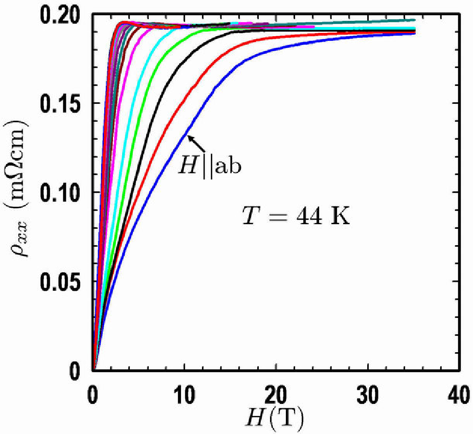
It is clearly seen that the anisotropy as $\gamma=H_{c2}^{\|}/H_{c2}^{\perp}$ decreases when calculated at lower resistive transitions. At the same time $H_{c2}^{90\%}(\theta)$ shown in Fig. 14 notably departures from the standard Ginzburg-Landau formula:

where $\gamma=(m_{c}/m_{a})^{1/2}$ is defined by the ratio of effective masses along the ab plane and the c-axis. The fit to Eq. (3) yields $\gamma\approx 8.9$ in this case. Data taken at 50 % and 10 % departure from Eq. (3) even stronger, which may result from increasing contribution of TAFF transport at lower resistivities.

The temperature dependencies of $\gamma(T)$ obtained from the $H_{c2}$ data shown in Figs. 8 and 9 for $H_{10}$, $H_{50}$ and $H_{c2}$ are shown in Fig. 15. Contrary to the standard one-band behavior, $\gamma$ turns out to be temperature dependent, the values of $\gamma_{10}(T)$, $\gamma_{50}(T)$ and $\gamma(T)$ being rather different, especially just below $T_{c}$. While the parameter of $H_{c2}$ anisotropy, $\gamma(T)=H_{c2}^{||}/H_{c2}^{\perp}$ decreases from $\approx 9$ at $T_{c}$ to $\approx 5$ at 34 K, the field $H_{10}$ becomes more anisotropic upon decreasing $T$. Below $T\approx 38$ K, however, these values of $\gamma(T)$ converge.

To understand how different pairing scenarios could manifest themselves in the observed temperature dependencies of $H_{c2}(T)$, we use the two-band BCS theory in which $T_{c}$ for interband scattering is given by [47, 48]

where $\lambda_{\pm}=\lambda_{11}\pm\lambda_{22}$, $w=\lambda_{11}\lambda_{22}-\lambda_{12}\lambda_{21}$, $s=\mbox{sign}(w)$, and $\lambda_{0}=(\lambda_{-}^{2}+4\lambda_{12}\lambda_{21})^{1/2}$, $\lambda_{12}$ and $\lambda_{22}$ are pairing constants in bands 1 and 2, and $\lambda_{12}$ and $\lambda_{21}$ quantify interband coupling. For s-wave pairing, intraband impurity scattering does not affect $T_{c0}$, while weak interband scattering reduces $T_{c}$ according to [50, 49, 26]

where $\gamma_{\pm}=\gamma_{12}\pm\gamma_{21}$, and $\gamma_{12}$ and $\gamma_{21}$ are scattering rates between bands 1 and 2, $N_{1}\gamma_{12}=N_{2}\gamma_{21}$ and $N_{1}\lambda_{12}=N_{2}\lambda_{21}$, where $N_{1}$ and $N_{2}$ are partial densities of states in bands 1 and 2, respectively. In the following we discuss two scenarios: 1. Conventional s-wave pairing dominated by strong intraband coupling, $w>0$. 2. Strong interband pairing $w<0$ which can result in the $\pi$ shift between the order parameters on two bands for interband repulsion $\lambda_{12}<0$ ($s^{\pm}$ pairing [15]).

As follows from Eq. (5), interband repulsion with $\lambda_{12}<0$ and $\lambda_{21}<0$ enhances $T_{c}$ depression due to interband impurity scattering between different pieces of the Fermi surface with opposite signs of the order parameter. This suppression may be reduced by strong coupling effects [51]. By contrast, for strong interband attraction, $4\lambda_{12}\lambda_{21}\gg\lambda_{-}^{2}$, Eq. (5) yields

Here $T_{c}$ suppression is much weaker than for the $s^{\pm}$ pairing because the factor $(1-\sqrt{N_{1}/N_{2}})^{2}$ reduces the effect of interband scattering, making $T_{c}$ independent of $\gamma_{12}$ in the special case of $N_{1}=N_{2}$. For instance, for $N_{1}=1.2N_{2}$, Eq. (6) gives a rather weak suppression of $T_{c}\simeq T_{c0}(1-0.02g)$ even in the dirty limit, $g=\gamma_{12}/2\pi T_{c0}>1$.

In the dirty limit, the equation for $H_{c2}$, which takes into account both orbital and Zeeman pairbreaking for negligible interband scattering, can be written in the following parametric form [26]:

where $t=T/T_{c0}$, and the functions $U_{1,2}$ are defined by

$\psi(x)$ is the di-gamma function, $D_{1}$ and $D_{2}$ are diffusivities in band 1 and 2, $D_{0}=\hbar/2m$, and the parameter $h$ runs from $0$ to $\infty$ as $T$ varies from $T_{c}$ to 0. For equal diffusivities, $\eta=D_{2}/D_{1}=1$, and negligible Zeeman pairbreaking, $D_{0}\ll D_{1,2}$, Eq. (8) simplifies to the one-band de-Gennes-Maki equation, $\ln t+U(h)=0$. If the magnetic field H is inclined by the angle $\theta$ with respect to the ab planes, Eqs. (8)-(9) also describe the angular dependence of $H_{c2}(\theta)$ if the intraband diffusivities are replaced by their angular-dependent values:

where $m=1,2$, and $D_{m}^{(a)}$ and $D_{m}^{(c)}$ are the in-plane and the c-axis principal values of $D_{m}^{\alpha\beta}$.

$H_{c2}(T)$ curves shown in Fig. 8 and 9 exhibit pronounced upward curvature for the field along the c-axis, and the downward curvature for the field along the ab plane, similar to the behavior of $H_{c2}(T)$ first observed on polycrystalline LaO_0.89F_0.11FeAs [7]. Such temperature dependence of $H_{c2}(T)$ has been often observed on MgB₂, suggesting that the two-band theory in which two bands have different diffusivities can also be used to describe $H_{c2}(T)$ in oxypnictides (the superconducting gaps on the disconnected pieces of the Fermi surface can be either different or the same). If interband scattering is negligible, neither $T_{c}$ nor $H_{c2}$ depend on the sign of $\lambda_{12}$, so we consider two different cases: 1. dominant intraband coupling, $w=\lambda_{11}\lambda_{22}-\lambda_{12}\lambda_{21}>0$ and 2. dominant interband coupling, $w=\lambda_{11}\lambda_{22}-\lambda_{12}\lambda_{21}<0$.

Shown in Fig. 16(a) is an example of the fit of Eq. (8)-(9) to the data for case 1 with $\lambda_{11}=\lambda_{22}=0.5$, and $\lambda_{12}=\lambda_{21}=0.25$, in which case $T_{c}=\Omega\exp[-1/(\lambda_{11}+\lambda_{12})]=50$K corresponds to $\Omega\simeq 190$K. Fig. 16(a) shows the fit without taking paramagnetic effects into account for $D_{2}=0.08D_{1}$, which suggests that scattering in one band is significantly stronger than in the other. We do not discuss here microscopic mechanisms behind such band disparity; instead we focus on the set of parameters which fit the data and the extent to which these parameters are different for the case of $w>0$ and $w<0$. Extrapolations of $H_{c2}^{\|}(T)$ to $T=0$ based on the observed slope at $T_{c}$ suggests $H_{c2}^{\|}(0)\sim\mathrm{\mathrm{\mathrm{}}}220$T, well above the weak coupling BCS paramagnetic limit $H_{p}[$T$]=1.84T_{c}[$K$]\simeq 90$T.

Fig. 16(a) shows the fit in the case of strong interband pairing $\lambda_{12}\lambda_{21}>\lambda_{11}\lambda_{21}$ for $\lambda_{11}=\lambda_{22}=0.49$, $\lambda_{12}=\lambda_{21}=0.5$ and $D_{2}^{a}=0.007D_{1}^{a}$. Reproducing the observed upward curvature of $H_{c2}^{\perp}(T)$ for this case requires a much greater disparity of the band diffusivities than for the previous case. Reducing $\lambda_{11}$ and $\lambda_{22}$ shifts the region of upward curvature to lower temperatures, which makes fitting the data even more difficult. These features may put serious constraints on the $s^{\pm}$ pairing scenario.

Given the very high extrapolated values of $H_{c2}^{\|}(0)$ in Fig. 16(a), the role of paramagnetic effects becomes very important. Shown in Fig. 16(c) is the fit for the same parameters as in Fig. 16(a) but with the account of the Zeeman pairbreaking for $D_{1}^{(a)}=10D_{0}$ and $[D_{2}^{(a)}D_{2}^{(c)}/D_{1}^{(a)}D_{1}^{(c)}]^{1/2}=0.7D_{0}$. In this case the values of $H_{c2}(T)$ at low temperatures are significantly reduced as compared to what may be expected from the fit in Fig. 16(a), which ignores the paramagnetic effects.

Several remarks should be made regarding the fits in Fig. 16(a-c). First, applying weak coupling Eqs. (8)-(9) for a superconductors with $T_{c}=50$ K obviously neglects the strong coupling renormalization effects of the Eliashberg theory. However given the lack of microscopic theory of superconductivity in oxypnictides, the use of the BCS-type approach may have its own merits given that the shape of the $H_{c2}(T)$ curve described by Eqs. (8)-(9) depends only on the ratio of the constants $\lambda_{mn}$ but it is basically insensitive to the particular s-wave pairing mechanisms. The usual way of treating strong coupling effects in Eqs. (8)-(9) is to express them in terms of experimentally observed parameters [52] such as $T_{c}$ and $D_{1}$ and $D_{2}$ extracted from normal state transport measurements and the observed slopes $dH_{c2}/dT$. The second remark is that the actual paramagnetic limit $H_{p}\simeq(1+\lambda)H_{p}^{BCS}$ is significantly enhanced by strong coupling effects as compared to the BCS value [53]. Here $\lambda\sim 1$ is a characteristic bare coupling constant for the relevant exchange boson, so $H_{c2}(T)$ values may significantly exceed $H_{p}^{BCS}$ as has been observed in other superconductors, for example PbMo₆S₈ [54, 55]. Thus, Eqs. (8)-(9) may capture the qualitative behavior of $H_{c2}(T)$ as functions of materials parameters if they are expressed in terms of the observed quantities, and the Zeeman terms are renormalized by strong coupling effects.

Our high-field data obtained on a Nd(O_1-xF_x)FeAs single crystals show extremely high $H_{c2}$ values, consistent with previous low-field measurements on single crystals [3, 36, 34, 33, 35] and high-field measurements on polycrystals [7, 8]. Our values of the temperature-dependent $H_{c2}$ slopes, $H_{c2}^{\prime\|}\approx 8-10$ T/K and $H_{c2}^{\prime\perp}\approx 1.2-5$ T/K measured from the resistivity onset of superconductivity are considerably higher than the values of $H_{c2}$ extracted from calorimetry measurements on Nd(O_1-xF_x)FeAs single crystals [36], which may be affected by strong paramagnetism of Nd³⁺ ions at high fields [10]. We should also mention several issues, which may complicate accurate extraction of the anisotropy in Nd(O_1-xF_x)FeAs single crystals grown by the flux method, which usually results in intergrowths and stacking faults parallel to the ab plane. Such planar defects may increase the apparent anisotropy parameter $\gamma$ and give rise to the local modulations of order parameter along the c-axis. The latter may broaden the resistive transition at $T_{c}$ and the upward curvature of $H_{c2}(T)$ near $T_{c}$, which could mask the two-band effects.

Because of very high values of $H_{c2}^{\prime\|}$ and $H_{c2}^{\prime\perp}$, our high field measurements up to 60 T are still mostly limited to the temperatures not too far from $T_{c}$, particularly for the field parallel to the ab plane. As a result, it is hard to unambiguously evaluate the values $H_{c2}(0)$, as Figs. 16(a-c) illustrate. Yet we can evaluate the in-plane and the c-axis GL coherence lengths, $\xi_{a}=(\phi_{0}/2\pi H_{c2}^{\prime\perp}T_{c})^{1/2}\simeq 2.3$ nm and $\xi_{c}=\xi_{a}/\gamma=0.26$ nm for $\gamma=9$, $H_{c2\perp}^{\prime}=1.2$ T/K and $T_{c}=50$ K. These values of $\xi_{a}$ and $\xi_{c}$ are not too different from those for YBa₂Cu₃O_7-x. The fits shown in Figs. 16(a-c) also indicate the importance of paramagnetic effects in $H_{c2}(T)$, particularly the fact that extrapolations of $H_{c2}$ to low temperatures based on the measured slope $H_{c2}^{\prime}$ and the WHH formula $H_{c2}\simeq 0.7T_{c}H_{c2}^{\prime}$ [5] may grossly overestimate $H_{c2}(0)$. At the same time, the importance of paramagnetic effects in oxypnictides might open up possibilities of observing first order phase transitions or perhaps the Fulde-Ferrel-Larkin-Ovchinnikov inhomogeneous states at very high magnetic fields.

The temperature dependence of $H_{c2}^{\perp}(T)$ shown in Fig. 9 is rather different from the conventional one-band WHH behavior, which may be characteristic of many oxypnictides. This confirms our earlier qualitative conclusion inferred from indirect measurements of $H_{c2}^{\perp}(T)$ on polycrystalline oxypnictides [7]. One possibility to explain the significant upward curvature of $H_{c2}^{\perp}(T)$ is based on the two-band model. This conclusion is also consistent with the temperature dependent mass anisotropy parameter, $\gamma(T)$, reminiscent of the behavior of MgB₂ [26, 56]. Yet many important points remains controversial. First, to explain the observed upward curvature of $H_{c2}^{\perp}(T)$, we had to assume a rather high difference in the intraband diffusivities, $D_{2}\sim(0.1-0.01)D_{1}$ (depending on the pairing scenario), considerably higher than the effective mass difference for $\Gamma$ and $M$ electron pockets predicted by ab-initio calculations [16, 17, 18, 19]. One has therefore to assume that scattering on impurities or strong magnetic excitations may produce such big differences in $D_{1}$ and $D_{2}$.

Our data enable us to make further qualitative conclusions regarding the s-wave two-band pairing scenarios with and without the interband $\pi$ shift. The first one is less susceptible to the pairbreaking effect of interband impurity scattering, as follows from Eqs. (5) and (6). Indeed, the fact that our Nd(O,F)FeAs single crystal has the same $T_{c}$ as sintered multiphase polycrystals, seems to suggest that the impurity scattering does not suppress $T_{c}$ much. The latter may also indicate that oxypnictides are effectively in the clean limit just because of their short coherence lengths, $\xi_{a}<\ell$, where $\ell$ is the mean free path. Yet $s^{\pm}$ pairing is certainly more susceptible to the pairbreaking interband impurity scattering. Another indication that the s-wave pairing without the interband $\pi$ shift appears to fit our data better comes from the fact that, in order to explain the observed upward curvature of $H_{c2}^{\perp}(T)$ in Fig. 16(b) in the $s^{\pm}$ model, we have to assume the ratio $D_{1}/D_{2}$ to be about an order of magnitude smaller that $D_{2}/D_{1}\sim 0.1$ required for the more traditional model of strong intraband pairing and weaker interband pairing. These constraints may reduce the number of possible scenarios of superconductivity in the oxypnictides.

As far as vortex dynamics in Nb(F,O)FeAs is concerned, our data presented in Figs. 3 and 4 show that high magnetic fields parallel to the c-axis mostly shift the resistive transition without significant broadening of the $\rho_{xx}(T)$ curves, while $H$ parallel to the ab plane changes the shape of $\rho_{xx}(T)$, but certainly not as strong as for high-$T_{c}$ cuprates [46]. This suggests that despite the rather high values of $\gamma$, thermal fluctuation of vortices in Nb(F,O)FeAs single crystals are weaker than in most anisotropic layered cuprates, like Bi-2212. This conclusion is consistent with the data of other groups [57] and with the relatively high activation energy $E_{0}\sim 3\times 10^{3}$ K extracted from our transport measurements. The effect of thermal fluctuations is also quantified by the Ginzburg parameter, $Gi=(2\pi k_{B}T_{c}\mu_{0}\Lambda_{0}^{2}/\phi_{0}^{2}\xi_{c})^{2}/2$, where $\Lambda_{0}$ is the in-plane London penetration depth. Taking $\Lambda_{0}=200$ nm, $\xi_{c}=0.26$ nm and $T_{c}=49$ K, we obtain $Gi\simeq 10^{-2}$, of the order of the typical Ginzburg number for YBCO. For two-band superconductors, the above estimates of $Gi$ remain qualitatively the same if $\gamma$ and $\xi$ are taken for the band with the minimum effective mass or maximum electron mobility [26]. By contrast, $Gi$ in La(O,F)FeAs is close to $Gi$ in MgB₂, about 30 times smaller than $Gi$ in Nd(O,F)FeAs [7, 8].

In conclusion, our high-field magneto-transport measurements on single crystal Nd(O_0.70F_0.30)FeAs have revealed very high upper critical fields and their anomalous temperature dependencies. We also observe a pronounced thermally-activated flux flow resistivity which may indicate rich vortex dynamics in single layer oxypnictides.

The work at NHMFL was supported by the NSF Cooperative Agreement No. DMR-0084173, by the State of Florida, by the DOE, by the NHMFL IHRP program (FH), and by AFOSR grant FA9550-06-1-0474 (AG and DCL).

References

- [1] Y. Kamihara, T. Watanabe, M. Hirano, and H. Hosono. J. Am. Chem. Soc. 130, 3296 (2008).
- [2] H. Takahashi, K. Igawa, K. Arii, Y. Kamihara, M. Hirano, and H. Hosono. Nature 453, 376 (2008).
- [3] C. Martin, R. T. Gordon, M. A. Tanatar, M. D. Vannette, M. E. Tillman, E. D. Mun, P. C. Canfield, V. G. Kogan, G. D. Samolyuk, J. Schmalian, et al. (2008), arXiv.org:0807.0876.
- [4] J. D. Moore, K. Morrison, K. A. Yates, A. D. Caplin, Y. Yeshurun, L. F. Cohen, J. M. Perkins, C. M. McGilvery, D. W. McComb, Z. A. Ren, et al. Supercond. Sci. Technol. 21, 092004 (2008).
- [5] C. Senatore, R. Flükiger, M. Cantoni, G. Wu, R. H. Liu, and X. H. Chen. Phys. Rev. B 78, 054514 (2008).
- [6] X. L. Wang, S. R. Ghorbani, S. X. Dou, X.-L. Shen, W. Yi, Z.-C. Li, and Z.-A. Ren (2008), arXiv.org:0806.1318, unpublished.
- [7] F. Hunte, J. Jaroszynski, A. Gurevich, D. C. Larbalestier, R. Jin, A. S. Sefat, M. A. McGuire, B. C. Sales, D. K. Christen, and D. Mandrus. Nature 453, 903 (2008).
- [8] J. Jaroszynski, S. C. Riggs, F. Hunte, A. Gurevich, D. C. Larbalestier, G. S. Beobinger, F. F. Balakirev, A. Migliori, Z. A. Ren, W. Lu, et al. Physical Review B 78, 064511 (2008).
- [9] T. Yildirim. Phys. Rev. Lett. 101 (2008).
- [10] C. Tarantini, A. Gurevich, D. C. Larbalestier, Z. A. Ren, X. L. Dong, W. Lu, and Z. X. Zhao (2008), arXiv.org:0805.4445, unpublished.
- [11] J. Wu, P. Phillips, and A. H. C. Neto. Phys. Rev. Lett. 101, 126401 (2008).
- [12] A. Yamamoto, J. Jiang, C. Tarantini, N. Craig, A. A. Polyanskii, F. Kametani, F. Hunte, J. Jaroszynski, E. E. Hellstrom, D. C. Larbalestier, et al. Appl. Phys. Lett. 92, 252501 (2008a).
- [13] A. Yamamoto, A. Polyanskii, J. Jiang, F. Kametani, C. Tarantini, F. Hunte, J. Jaroszynski, E. Hellstrom, P. Lee, A. Gurevich, et al. Superconductor Science and Technology 21, 095008 (2008b).
- [14] R. Prozorov, M. E. Tillman, E. D. Mun, and P. C. Canfield (2008), arXiv.org:0805.2783, unpublished.
- [15] I. I. Mazin, D. J. Singh, M. D. Johannes, and M. H. Du. Phys. Rev. Lett. 101, 057003 (2008).
- [16] D. J. Singh and M. H. Du. Phys. Rev. Lett. 100 (2008).
- [17] S. Raghu, X.-L. Qi, C.-X. Liu, D. J. Scalapino, and S.-C. Zhang. Phys. Rev. B 77, 220503 (2008).
- [18] S. Graser, G. R. Boyd, C. Cao, H.-P. Cheng, P. J. Hirschfeld, and D. J. Scalapino. Phys. Rev. B 77, 180514 (2008).
- [19] S. Ishibashi, K. Terakura, and H. Hosono. J. Phys. Soc. Jap. 77, 053709 (2008).
- [20] R. H. T. Wilke, S. L. Bud’ko, P. C. Canfield, D. K. Finnemore, R. J. Suplinskas, and S. T. Hannahs. Phys. Rev. Lett. 92, 217003 (2004).
- [21] L. Lyard, P. Szabó, T. Klein, J. Marcus, C. Marcenat, K. H. Kim, B. W. Kang, H. S. Lee, and S. I. Lee. Phys. Rev. Lett. 92, 057001 (2004).
- [22] A. Rydh, U. Welp, A. E. Koshelev, W. K. Kwok, G. W. Crabtree, R. Brusetti, L. Lyard, T. Klein, C. Marcenat, B. Kang, et al. Phys. Rev. B 70, 132503 (2004).
- [23] V. Braccini, A. Gurevich, J. E. Giencke, M. C. Jewell, C. B. Eom, D. C. Larbalestier, A. Pogrebnyakov, Y. Cui, B. T. Liu, Y. F. Hu, et al. Phys. Rev. B 71, 012504 (2005).
- [24] M. Angst, S. L. Bud’ko, R. H. T. Wilke, and P. C. Canfield. Phys. Rev. B 71, 144512 (2005).
- [25] H.-J. Kim, H.-S. Lee, B. Kang, W.-H. Yim, Y. Jo, M.-H. Jung, and S.-I. Lee. Phys. Rev. B 73, 064520 (pages 5) (2006).
- [26] A. Gurevich. Physica C 456, 160 (2007), phys. Rev. B 67, 184515 (2003).
- [27] S. L. Bud’ko and P. C. Canfield. Phys. Rev. B 65, 212501 (2002), S.L. Bud’ko, P.C. Canfield, V.G. Kogan. Physica C 387, 85 (2002).
- [28] V. Ferrando, P. Manfrinetti, D. Marré, M. Putti, I. Sheikin, C. Tarantini, and C. Ferdeghini. Phys. Rev. B 68, 094517 (2003).
- [29] E. Ohmichi, T. Masui, S. Lee, S. Tajima, and T. Osada. J. Phys. Soc. Japan 73, 2065 (2004).
- [30] A. Gurevich, S. Patnaik, V. Braccini, K. H. Kim, C. Mielke, X. Song, L. D. Cooley, S. D. Bu, D. M. Kim, J. H. Choi, et al. Supercond. Sci. Technol. 17, 278 (2004).
- [31] A. V. Pogrebnyakov, X. X. Xi, J. M. Redwing, V. Vaithyanathan, D. G. Schlom, A. Soukiassian, S. B. Mi, C. L. Jia, J. E. Giencke, C. B. Eom, et al. Appl. Phys. Lett. 85, 2017 (2004).
- [32] P. S. P. Samuely, Z. Holanova, S. Budko, and P. Canfield. Physica C 435, 71 (1959).
- [33] Y. Jia, P. Cheng, L. Fang, H. Luo, H. Yang, C. Ren, L. Shan, C. Gu, and H.-H. Wen. Applied Physics Letters 93, 032503 (2008a).
- [34] P. Cheng, H. Yang, Y. Jia, L. Fang, X. Zhu, G. Mu, and H.-H. Wen (2008), arXiv.org:0806.1668, unpublished.
- [35] Y. Jia, P. Cheng, L. Fang, H. Yang, C. Ren, L. Shan, C.-Z. Gu, and H.-H. Wen. Supercond. Sci. Technol. p. 105018 (2008b).
- [36] U. Welp, R. Xie, A. E. Koshelev, W. K. Kwok, P. Cheng, L. Fang, and H. H. Wen (2008), arXiv.org:0807.4196, unpublished.
- [37] N. R. Werthamer, E. Helfand, and P. C. Hohenberg. Phys. Rev. 147, 295 (1966).
- [38] P. Lindqvist, A. Nordström, and O. Rapp. Phys. Rev. Lett. 64, 2941 (1990), Phys. Rev. B 45, 12577–12579 (1992).
- [39] P. Santhanam, C. C. Chi, S. J. Wind, M. J. Brady, and J. J. Bucchignano. Phys. Rev. Lett. 66, 2254 (1991).
- [40] C. Strunk, V. Bruyndoncx, C. Van Haesendonck, V. V. Moshchalkov, Y. Bruynseraede, C.-J. Chien, B. Burk, and V. Chandrasekhar. Phys. Rev. B 57, 10854 (1998).
- [41] R. Vaglio, C. Attanasio, L. Maritato, and A. Ruosi. Phys. Rev. B 47, 15302 (1993), C. Attanasio, S. Barbenera, T. Di Luccio, S.L. Prischepa, R. Russo, M. Salvato, and L. Maritato, J. Phys. Cond. Mat. 13, 3215 (2001).
- [42] M. Sawicki, T. Dietl, J. Kossut, J. Igalson, T. Wojtowicz, and W. Plesiewicz. Phys. Rev. Lett. 56, 508 (1986).
- [43] I. P. Smorchkova, N. Samarth, J. M. Kikkawa, and D. D. Awschalom. Phys. Rev. Lett. 78, 3571 (1997).
- [44] T. Andrearczyk, J. Jaroszyński, G. Grabecki, T. Dietl, T. Fukumura, and M. Kawasaki. Phys. Rev. B 72, 121309 (2005).
- [45] B. L. Al’tshuler and A. G. Aronov, in Electron-Electron Interactions in Disordered Systems, edited by A. L. Efros and M. Pollak (North Holland, Amsterdam, 1985), p. 1, H. Fukuyama, ibid, p. 155; P. A. Lee and T. V. Ramakrishnan, Rev. Mod. Phys. 57, 287 (1985).
- [46] G. Blatter, M. V. Feigel’man, V. B. Geshkenbein, A. I. Larkin, and V. M. Vinokur. Rev. Mod. Phys. 66, 1125 (1994).
- [47] H. Suhl, B. T. Matthias, and L. R. Walker. Phys. Rev. Lett. 3, 552 (1959).
- [48] V. Moskalenko. Fiz. Met. Metalloved. 8, 503 (1959), [Sov. Phys. Met. Metallog. 8, 25 (1959)].
- [49] A. A. Golubov and I. I. Mazin. Phys. Rev. B 55, 15146 (1997).
- [50] N. Schophol and K. Scharnberg. Solid State Comm. 22, 371 (1977).
- [51] Y. Senga and H. Kontani (2008), arXiv.org:0809.0374, unpublished.
- [52] J. A. X. Alexander, T. P. Orlando, D. Rainer, and P. M. Tedrow. Phys. Rev. B 31, 5811 (1985).
- [53] M. Schossmann and J. P. Carbotte. Phys. Rev. B 39, 4210 (1989).
- [54] Ø. Fisher. Appl. Phys. 16, 1 (1978).
- [55] H. J. Niu and D. P. Hampshire. Phys. Rev. B 69, 174503 (2004).
- [56] P. Canfield, S. Bud’ko, and D. Finnemore. Physica C 385, 1 (2003).
- [57] H. Yang, C. Ren, L. Shan, and H.-H. Wen. Phys. Rev. B 78, 092504 (2008).