Two-dimensional spanning webs as (1,2) logarithmic minimal model

We begin with the examination of the determinant expansion of the usual Laplace matrix $\Delta$ for the graph $\mathcal{G}$. Let the vertices of the set $V$ be labeled in arbitrarily order from 1 to $n=|V|=MN$. Then $\Delta$ has the elements ($i,j\in\{1,\ldots,n\}$)

where $z_{i}$ is the order of vertex $i$. Since the matrix $\Delta$ has a zero eigenvalue, its determinant vanishes. On the other hand, the Leibniz formula expresses the determinant of $\Delta$ as a sum over all permutations $\sigma$ of the set $\{1,2,\dots,n\}$:

where $S_{n}$ is the symmetric group, $\mathrm{sgn}(\sigma)=\pm 1$ is the signature of the permutation $\sigma$. The identity permutation $\sigma=\sigma_{\mathrm{id}}$ in (2) yields the term $z_{1}z_{2}\cdots z_{n}$ equal to the number of all possible arrow configurations on $\mathcal{G}$.

In general, each permutation $\sigma\in S_{n}$ can be factored into a product (composition) of disjoint cyclic permutations, say, $\sigma=c_{1}\circ c_{2}\cdots\circ c_{k}$. This representation partitions the set of vertices $V$ into non-empty disjoint subsets - the orbits $\mathcal{O}_{i}$ of the corresponding cycles $c_{i}$, $i=1,\dots,k$. More precisely, if $\mathcal{O}_{i}=\{v_{i,1},v_{i,2},\dots v_{i,l_{i}}\}\subset V$ is the orbit of $c_{i}$, then $\cup_{i=1}^{k}\mathcal{O}_{i}=V$ and $\sum_{i=1}^{k}l_{i}=n$, where $l_{i}$ is the cardinality of the orbit $\mathcal{O}_{i}$, equivalently, the length of the cycle $c_{i}$. The orbits consisting of just one element, if any, constitute the set $S_{fp}(\sigma)$ of fixed points of the permutation: $S_{fp}(\sigma)=\{v=\sigma(v),v\in V\}$. In the case of the identity permutation $\sigma_{\mathrm{id}}\in S_{n}$ all orbits consist of exactly one element, $\mathcal{O}_{i}(\sigma_{\mathrm{id}})=\{v_{i}\}\subset V$, $i=1,\dots,n$, and $S_{fp}(\sigma_{\mathrm{id}})=V$. A cycle $c_{i}$ of length $|c_{i}|=l_{i}\geq 2$ will be called a proper cycle. A proper cycle of length 2 corresponds to two oppositely directed edges which connect a pair of adjacent vertices: $(v_{i,1}\rightarrow v_{i,2})$, $(v_{i,2}\rightarrow v_{i,1})$. Note that the vertices of an orbit $\mathcal{O}_{i}$ of cardinality $l_{i}=|O_{i}(\sigma)|\geq 3$ are connected by a closed path on $\mathcal{G}$ which can be traversed in two opposite directions: if $c_{i}$ is the cycle defined by $v_{i,1}\rightarrow\sigma(v_{i,1})=v_{i,2},\rightarrow\dots\rightarrow\sigma(v_{i,l_{i}})=v_{i,1}$, then the reverse cycle $c^{\prime}_{i}$ can be represented as $v_{i,l_{i}}\rightarrow\sigma(v_{i,l_{i}})=v_{i,l_{i}-1},\rightarrow\dots\rightarrow\sigma(v_{i,1})=v_{i,l_{i}}$.

Now we take into account that the proper cycles on $\mathcal{G}$ are of even length only, hence, the signature of every permutation in the expansion of the determinant depends on the number of proper cycles in its factorization, i.e., if $\sigma=c_{1}\circ c_{2}\cdots\circ c_{p}$, where $|c_{i}|\geq 2$, $i=1,\dots,p$, then $\mathrm{sgn}(\sigma)=(-1)^{p}$. Thus, the terms in Eq. (2) can be rearranged according to the number $p$ of disjoint proper cycles as follows:

Here $c_{i}^{k}$ is the $k$-fold composition of the cyclic permutation $c_{i}$ of even length $l_{i}$, $v_{i}\in\mathcal{O}_{i}(\sigma)$, so that $c_{i}^{k-1}(v_{i})\not=c_{i}^{k}(v_{i})$ and $c_{i}^{l_{i}}(v_{i})=v_{i}$. Note that all non-vanishing off-diagonal elements are equal to $-1$.

The above expansion reveals the following features: (i) As expected, all spanning digraphs on $\mathcal{G}$ have at least one proper cycle; (ii) Each term on the right-hand side with $S_{fp}(\sigma)\not=\emptyset$ represents a set of $\prod_{j\in S_{fp}}z_{j}$ distinct spanning digraphs which have in common the specified cycles $c_{1},\dots,c_{p}$, and differ in the oriented edges outgoing from the vertices $j\in S_{fp}(\sigma)$. These oriented edges may form cycles on their own which do not enter into the list $c_{1},\dots,c_{p}$; (iii) Since the sets $\cup_{i=1}^{p}\mathcal{O}_{i}$ and $S_{fp}(c_{1},\dots,c_{p})$ are disjoint, the proper cycles formed by the oriented edges incident to the fixed points of a given permutation $\sigma=c_{1}\circ c_{2}\circ\cdots\circ c_{p}$ should enter into the enlarged list of cycles $c_{1},c_{2},\dots,c_{p},\dots,c_{p^{\prime}}$, $p^{\prime}>p$, corresponding to the cycle decomposition of another permutation $\sigma^{\prime}$.

For example, consider the determinant of the Laplacian matrix of a cylinder of height 3 and perimeter 4. In the case of closed boundary conditions, the corresponding Leibniz expansion will contain the term

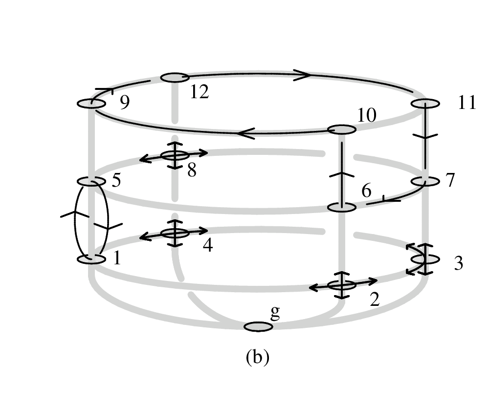
which represents, up to the sign, $z_{2}z_{6}=12$ spanning digraphs on $\mathcal{G}$ with 3 specified cycles and all possible oriented bonds outgoing from the vertices 2 and 6, as illustrated in Fig. 1 (a). One of these 12 spanning digraphs will contain the additional cycle $2\rightarrow 6\rightarrow 2$. In the case of open boundary at the bottom and closed at the top, the term

represents $z_{2}z_{3}z_{4}z_{8}=256$ spanning digraphs on $\mathcal{G}^{\prime}$ with 2 specified cycles and all possible oriented bonds outgoing from the vertices 2, 3, 4 and 8, as illustrated in Fig. 1 (b). The latter bonds will generate three digraphs with one additional cycle of length 2: $2\rightarrow 3\rightarrow 2$, or $3\rightarrow 4\rightarrow 3$, or $4\rightarrow 8\rightarrow 4$, and one digraph with two additional cycles, $2\rightarrow 3\rightarrow 2$ and $4\rightarrow 8\rightarrow 4$.

As noticed first in [19], the expansion (3) parallels in form the inclusion-exclusion principle in combinatorial mathematics. Indeed, let $c_{1},c_{2},\dots,c_{m}$ be the list of all possible proper cycles on $\mathcal{G}$, labeled in an arbitrary order. Define $A_{i}$, $i=1,2,\dots,m$ as the set of all spanning digraphs on $\mathcal{G}$ containing the particular cycle $c_{i}$. Then, expansion (3) can be written in the form of the inclusion-exclusion principle:

which holds for any finite sets $A_{1},A_{2},\dots,A_{m}$, where $|A|$ is the cardinality of the set $A$.

Now we are in the position to define a matrix $D^{(0,0)}$, associated with the graph $\mathcal{G}$, such that $\det D^{(0,0)}$ be the generating function of all spanning digraphs on $\mathcal{G}$ which have no contractible cycles. The elements $D_{ij}^{(0,0)},i,j=1,\dots,n=NM$ of $D^{(0,0)}$ are explicitly given as:

Here $a=\omega^{1/M}e^{-i\pi/M}$, the terms ”left” and ”right” fix the opposite directions of the horizontal edges. Note that all closed paths which do not wrap the cylinder contain an equal number of horizontal edges with either orientations, hence, their weight in $\det D^{(0,0)}$ remains the same as in $\det\Delta$. Therefore, all the configurations which contain such closed paths (contractible cycles) cancel out in the expansion of $\det D^{(0,0)}$. On the other hand, cycles generated by off-diagonal elements that wrap the cylinder change their sign, because they contain horizontal edges oriented in one direction exceeding by $M$ the number of edges in the opposite direction. This amounts to the total factor of $a^{M}=-\omega$, or $a^{-M}=-\omega^{-1}$ depending on the orientation. Therefore, each non-contractible cycle with a given orientation is counted twice, however, with different weight - once it enters into the determinant expansion with unit weight, being generated by diagonal elements of the matrix $D^{(0,0)}$, and second time it enters with a factor $\omega$ or $\omega^{-1}$ (depending on the orientation) as generated by off-diagonal elements of that matrix. Thus, the total number of non-contractible cycles, irrespective of their origin and orientation, is given by the coefficient in front of the corresponding power of $\omega+\omega^{-1}+2\equiv\xi$ in the series expansion of the partition function. The power of $\xi$ is the ”good quantum number” which is a well defined and conserved quantity under the action of the transfer matrix along the cylinder. However, as we shall see below, more convenient expansions of the partition function, which can be directly compared with characters of the Virasoro modules, are given by the power series in $\omega$ itself, or in terms of combinations like $(\omega+\omega^{-1})^{s}$ and $\sum_{k=0}^{s}\omega^{s-2k}$. In general, besides the non-contractible cycles, the spanning digraph contains tree subgraphs connected to them. All branches of the trees can be generated only by the diagonal elements of $D^{(0,0)}$ and, hence, carry unit weight.

The Laplacian matrix $\Delta^{\star}$ for the graph $\mathcal{G}^{\prime}$ corresponding to $(\mu,\nu)=(0,1)$ boundary conditions is a $(n+1)\times(n+1)$ matrix of the same form (1) as far as the notions of degree of a vertex and adjacency are understood in the context of $\mathcal{G}^{\prime}$. However, to make the similarities and dissimilarities with the former case apparent, we retain the notation $z_{i}$ for the degree of vertex $i$, $i=1,\dots,n$, with respect to $\mathcal{G}$, and explicitly introduce the label $g$ for the root with degree $M$ in $\mathcal{G}^{\prime}$, see Fig. (2) b. Thus, for the matrix elements of $\Delta^{\star}$ we have

Here $B$ is the set of bottom boundary vertices adjacent to the root $g$ in $\mathcal{G}^{\prime}$. Now we make use of the fact that by Kirchhoff’s theorem the number $N_{st}$ of spanning trees on $\mathcal{G}^{\prime}$ is equal to any cofactor of $\Delta^{\star}$ and chose for convenience the cofactor $C_{gg}$ of the element $\Delta^{\star}_{gg}$. Then $N_{st}=C_{gg}=\det\Delta^{\prime}$, where $\Delta^{\prime}$ is the $n\times n$ matrix with elements ($i,j=1,\dots,n$):

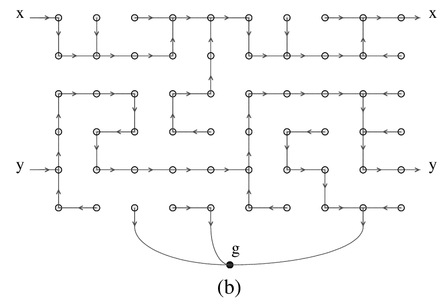
By comparing the above expression with (1) one sees that the only difference is in the diagonal elements: the order of the vertices belonging to the open boundary has been increased by one. Therefore, the same arguments as in the previous section lead us to the matrix $D^{(0,1)}$ with elements

where, as before, $a=\omega^{1/M}e^{-i\pi/M}$. By construction, in the expansion of $\det D^{(0,1)}$ all the arrow configurations with contractible cycles cancel out. Thus $\det D^{(0,1)}$ is the generating function of all the spanning digraphs which are either spanning forests of trees rooted at the open bottom boundary, or contain non-contractible cycles wrapping the cylinder and tree subgraphs rooted at these cycles or at the open boundary. As in the case of closed boundaries, each non-contractible cycle with a given orientation is counted twice with different weights - once with unit weight, being generated by diagonal elements of the matrix $D^{(0,1)}$, and second time with a factor $\omega$ or $\omega^{-1}$ (depending on the orientation) as generated by off-diagonal elements of that matrix.

The case of open-open boundary conditions, $(\mu,\nu)=(1,1)$, can be considered analogously to the previous two cases and we do not describe it separately.

The partition function calculated as the determinant of the Laplacian, $Z^{(\mu,\nu)}_{NM}=\det D^{(\mu,\nu)}$, can be split into a product of two parts,

where $e^{F^{(\mu,\nu)}_{NM}}$ is the nonuniversal part of the partition function, including bulk and boundary free energy $F^{(\mu,\nu)}_{NM}$, and $\bar{Z}^{(\mu,\nu)}_{N}(q,\omega)$ is the universal part which is a polynomial in the aspect ratio parameter $q=e^{-\frac{\pi M}{N}}$ and a Laurent polynomial in $\omega$. The universal part of the partition function can be decomposed into different combinations of $\omega$, for example,

valid for all boundary conditions under consideration, $\mu,\nu=0,1$. Note that the second and third polynomials can be obtained from the first one by using the relations:

Each of the polynomials $C^{(\mu,\nu)}_{i,s}[N](q)$, $i=1,2,3$, has a well defined statistical meaning. For example, $C^{(\mu,\nu)}_{1,s}[N](q)$ is the universal factor in the partition function which is proportional to the number of configurations with $s$ non-contractible cycles of either orientation, generated by off-diagonal elements of the matrix $D^{(\mu,\nu)}$; these configurations may have also any allowed (by the size of the cylinder) number of non-contractible cycles of both orientations, generated by diagonal elements of that matrix. On the other hand, the universal factor $C^{(\mu,\nu)}_{2,s}[N](q)$ is proportional to the number of configurations with fixed to $s$ difference in the numbers of non-contractible cycles with positive and negative orientation, generated by off-diagonal elements of the matrix $D^{(\mu,\nu)}$; the total number of such cycles, as well as the number of non-contractible cycles of either orientation, generated by diagonal elements of the same matrix, may take any allowed values.

In the next section, we shall evaluate the asymptotic form of the coefficients $C^{(\mu,\nu)}_{i,s}[N]$, $i=2,3$, for $M\rightarrow\infty$, $N\rightarrow\infty$ and disclose their relation to the finitized characters of the logarithmic Virasoro modules.

References

- [1] C. Kirchhoff, Ann. Phys. Chem. 72, 497 (1847).
- [2] C. Fan and F. Y. Wu, Phys. Rev. B2, 723 (1970).
- [3] D. Dhar, Phys. Rev. Lett. 64, 1613 (1990).
- [4] P. W. Kasteleyn, Physica 29, 1329 (1963).
- [5] H. Saleur, Nucl. Phys. B 382 486-531 (1992).
- [6] M. Gordon, P. Kapadia, and A. Malakis, J. Phys. A 9, 751 (1976).
- [7] P. W. Kasteleyn, Physica 27, 1209 (1961).
- [8] H. N. V. Temperley and M. E. Fisher, Philos. Mag. 6, 1061 (1961).
- [9] P. Ruelle, Phys. Lett. B 539, 172 (2002).
- [10] G. Piroux and P. Ruelle, Phys. Lett. B 607, 188 (2005).
- [11] M. Jeng, G. Piroux, and P. Ruelle, J. Stat. Mech.: Theor. Exp. P10015 (2006).
- [12] V. S. Poghosyan, S. Y. Grigorev, V. B. Priezzhev, and P.Ruelle, Phys. Lett. B 659, 768 (2008).
- [13] C. M. Fortuin and P. W. Kasteleyn, Physica 57, 536 (1972).
- [14] J. Bouttier, M. Bowick, E. Guitter, and M. Jeng, Phys. Rev. E 76, 041140 (2007).
- [15] V. S. Poghosyan, V. B. Priezzhev, and P. Ruelle, Phys. Rev. E 76, 041130 (2008).
- [16] N. Sh. Izmailian, V. B. Priezzhev, P. Ruelle, and C-K. Hu, Phys. Rev. Lett. 95, 260602 (2005).
- [17] P. A. Pearce, J. Rasmussen, and J-B. Zuber, J. Stat. Mech.: Theor. Exp., P11017 (2006).
- [18] P. A. Pearce and J. Rasmussen, J. Stat. Mech.: Theor. Exp., P02015 (2007).
- [19] V. B. Priezzhev, Sov. Phys. Usp. 28, 1125 (1985).
- [20] B. Feigin, E. Feigin, I. Tipunin, arXiv:0704.2464.
- [21] H.G. Kausch, Nucl. Phys. B 583, 513 (2000), arXiv:hep-th/0003029.
- [22] B. Feigin, I. Tipunin, arXiv:0805.4096.
- [23] R.E. Behrend, P.A. Pearce, V.B. Petkova, J.-B. Zuber, Nucl. Phys. B570 (2000) 525-589; Nucl.Phys. B579 (2000) 707-773; arXiv:hep-th/9908036.
- [24] P. A. Pearce, J. Rasmussen, and P. Ruelle, J. Phys. A: Math. Theor. 41, 295201 (2008).
- [25] S.N. Majumdar and D. Dhar, Physica A 185, 129 (1992).
- [26] G. Piroux, P. Ruelle, Phys. Lett. B 607, 188 (2005).