跳到论文正文
W Papers独立论文阅读器 arXiv:0810.2188 论文正文 计算阅读时间 · 0%
引用这篇论文根据当前论文元数据生成,正式投稿前建议核对。


License: arXiv.org perpetual non-exclusive license
arXiv:0810.2188v2 [math.CV] 10 May 2011

Discrete complex analysis on isoradial graphsThanks: A St.Petersburg Department of Steklov Mathematical Institute (PDMI RAS). Fontanka 27, 191023 St.Petersburg, Russia.Thanks: B Section de Mathématiques, Université de Genève. 2-4 rue du Lièvre, Case postale 64, 1211 Genève 4, Suisse.Thanks: C Chebyshev Laboratory, Department of Mathematics and Mechanics, Saint-Petersburg State University. 14th Line, 29b, 199178 Saint-Petersburg, Russia.Thanks: E-mail addresses: dchelkak@pdmi.ras.ru, Stanislav.Smirnov@unige.ch

Dmitry Chelkaka,c and Stanislav Smirnovb,c
Date: August 24, 2026
Abstract.

We study discrete complex analysis and potential theory on a large family of planar graphs, the so-called isoradial ones. Along with discrete analogues of several classical results, we prove uniform convergence of discrete harmonic measures, Green’s functions and Poisson kernels to their continuous counterparts. Among other applications, the results can be used to establish universality of the critical Ising and other lattice models.

Key words and phrases: 
Discrete harmonic functions, discrete holomorphic functions, discrete potential theory, isoradial graphs, random walk
1991 Mathematics Subject Classification
39A12, 52C20, 60G50

1. Introduction

1.1. Motivation

This paper is concerned with discrete versions of complex analysis and potential theory in the complex plane. There are many discretizations of harmonic and holomorphic functions, which have a long history. Besides proving discrete analogues of the usual complex analysis theorems, one can ask to which extent discrete objects approximate their continuous counterparts. This can be used to give “discrete” proofs of continuous theorems (see, e.g., [L-F55] for such a proof of the Riemann mapping theorem) or to prove convergence of discrete objects to continuous ones. One of the goals of our paper is to provide tools for establishing convergence of critical 2D lattice models to conformally invariant scaling limits.

There are no “canonical” discretizations of Laplace and Cauchy-Riemann operators, the most studied ones (and perhaps the most convenient) are for the square grid. There are also definitions for other regular lattices, as well as generalizations to larger families of embedded into ℂ{\mathbb{C}} planar graphs (see [Smi10b] and references therein).

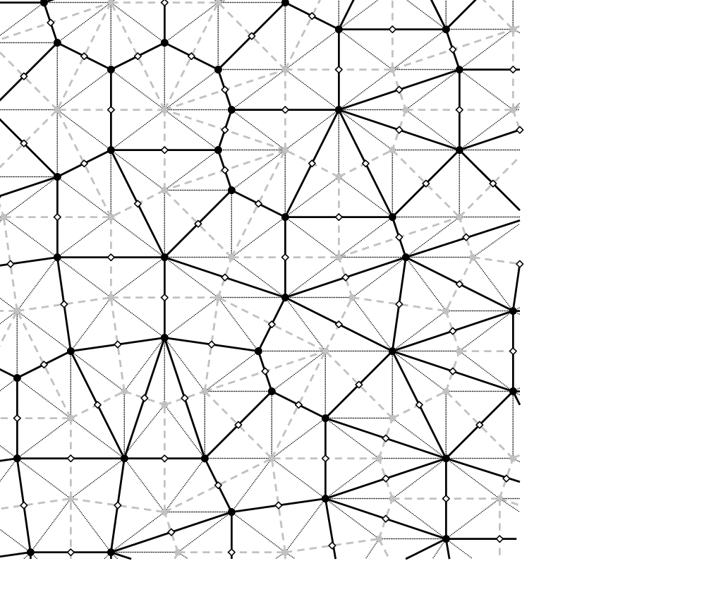
We will work with isoradial graphs (or, equivalently, rhombic lattices) where all faces can be inscribed into circles of equal radii. Rhombic lattices were introduced by R. J. Duffin [Duf68] in late sixties as (perhaps) the largest family of graphs for which the Cauchy-Riemann operator admits a nice discretization, similar to that for the square lattice. They reappeared recently as isoradial graphs in the work of Ch. Mercat [Mer01] and R. Kenyon [Ken02], as the largest family of graphs where certain 2D statistical mechanical models (notably the Ising and dimer models) preserve some integrability properties. Note that isoradial graphs can be quite irregular – see e.g. Fig. 1A. It was shown by R. Kenyon and J.-M. Schlenker [KS04] that many planar graphs admit isoradial embeddings – in fact, there are only two topological obstructions. Also isoradial graphs have a well-defined mesh size δ\delta – the common radius of the circumscribed circles.

It is thus natural to consider this family of graphs in the context of universality for 2D models with (conjecturally) conformally invariant scaling limits (as the mesh tends to zero).

The primary goal of our paper is to provide a “toolbox” of discrete versions of continuous results (particularly “hard” estimates) sufficient to perform a passage to the scaling limit. Of particular interest to us is the critical Ising model, and this paper starts a series devoted to its universality (which means that the scaling limit is independent of the shape of the lattice). See [Smi06], [CS08] for the strategy of our proof, [CS09] for the convergence of certain discrete holomorphic observables and [Smi10a] for the square lattice case.

Our results can also be applied to other lattice models. The uniform convergence of the discrete Poisson kernel (1.3) already implies universality for the loop-erased random walks on isoradial graphs. Namely, our paper together with [LSW04] implies that their trajectories converge to SLE(2)(2) curves (see Sect. 3.2, especially Remark 3.6, in [LSW04]). There are several other fields where discrete harmonic and discrete holomorphic functions defined on isoradial graphs play essential role and hence where our results may be useful: approximation of conformal maps [Bück08]; discrete integrable systems [BMS05]; and the theory of discrete Riemann surfaces [Mer07].

Local convergence of discrete harmonic (holomorphic) functions to continuous harmonic (holomorphic) functions is a rather simple fact. Moreover, it was shown by Ch. Mercat [Mer02] that each continuous holomorphic function can be approximated by discrete ones. Thus, the discrete theory is close to the continuous theory “locally.” Nevertheless, until recently almost nothing was known about the “global” convergence of the functions defined in discrete domains as the solutions of some discrete boundary value problems to their continuous counterparts. This setup goes back to the seminal paper by R. Courant, K. Friedrichs and H. Lewy [CFL28], where convergence is established for harmonic functions with smooth Dirichlet boundary conditions in smooth domains, discretized by the square lattice, but not much progress has occurred since. For us it is important to consider discrete domains with possibly very rough boundaries and to establish convergence without any regularity assumptions about them. Besides being of independent interest, this is indispensable for establishing convergence to Oded Schramm’s SLEs, since the latter curves are fractal.
Refer to caption

(A)

Refer to caption

(B)

Figure 1. (A) An isoradial graph Γ\Gamma (black vertices, solid lines), its dual isoradial graph Γ∗\Gamma^{*} (gray vertices, dashed lines), the corresponding rhombic lattice or quad-graph (vertices Λ=Γ∪Γ∗\Lambda=\Gamma\cup\Gamma^{*}, thin lines, rhombic faces) and the set ♢=Λ∗\diamondsuit=\Lambda^{*} of rhombi centers (diamond-shaped points). (B) Local notations near u∈Γu\in\Gamma. The dual face W⁡(u)W(u) is shaded.

1.2. Preliminary definitions.

The planar graph Γ\Gamma embedded in ℂ{\mathbb{C}} is called isoradial iff each face is inscribed into a circle of a common radius δ\delta. If all circle centers are inside the corresponding faces, then one can naturally embed the dual graph Γ∗\Gamma^{*} in ℂ{\mathbb{C}} isoradially with the same δ\delta, taking the circle centers as vertices of Γ∗\Gamma^{*}. The name rhombic lattice is due to the fact that all quadrilateral faces of the corresponding bipartite graph Λ\Lambda (having the vertex set Γ∪Γ∗\Gamma\cup\Gamma^{*}) are rhombi with sides of length δ\delta (see Fig. 1A). We will often work with rhombi half-angles, denoted by θ\theta, for which we also require the following mild but indispensable and widely used assumption (see, e.g., [Cia78], pp. 124 and 130, where the similar assumption is called Zlámal’s condition):

(♠\spadesuit) the rhombi half-angles are uniformly bounded from 00 and 12​π\frac{1}{2}\pi (in other words, all these angles belong to [η,12​π−η][\eta,\frac{1}{2}\pi-\eta] for some fixed η>0\eta>0), i.e., there are no “too flat” rhombi in Λ\Lambda.

Note that condition (♠\spadesuit)  implies that for each u1,u2∈Γu_{1},u_{2}\in\Gamma the Euclidean distance |u2−u1||u_{2}-u_{1}| and the combinatorial distance δ⋅dΓ​(u1,u2)\delta\cdot d_{\Gamma}(u_{1},u_{2}) (where dΓ​(u1,u2)d_{\Gamma}(u_{1},u_{2}) is the minimal number of vertices in the path connecting u1u_{1} and u2u_{2} in Γ\Gamma) are comparable. Below we often use the notation const for absolute positive constants that does not depend on the mesh δ\delta or the graph structure but, in principle, may depend on η\eta.

The function H:ΩΓδ→ℝH:\Omega^{\delta}_{\Gamma}\to{\mathbb{R}} defined on some subset (discrete domain) ΩΓδ\Omega^{\delta}_{\Gamma} of Γ\Gamma is called discrete harmonic, if

∑s=1ntan⁡θs⋅(H⁡(us)−H⁡(u))=0\sum_{s=1}^{n}\tan\theta_{s}\cdot(H(u_{s})\!-\!H(u))=0 (1.1)

at all u∈ΩΓδu\in\Omega^{\delta}_{\Gamma} where the left-hand side makes sense. Here θs\theta_{s} denotes the half-angles of the corresponding rhombi, see also Fig. 1B for notations. As usual, this definition is closely related to the random walk on Γ\Gamma such that the probability to make the next step from uu to uku_{k} is proportional to tan⁡θk\tan\theta_{k}. Namely, RW⁡(t+1)=RW⁡(t)+ξRW⁡(t)(t)\mathrm{RW}(t+1)=\mathrm{RW}(t)+\xi^{(t)}_{\mathrm{RW}(t)}, where the increments ξ(t)\xi^{(t)} are independent with distributions

𝐏⁡(ξu=uk−u)=tan⁡θk∑s=1ntan⁡θsfork=1,..,n.{\bf P}(\xi_{u}=u_{k}-u)=\frac{\tan\theta_{k}}{\sum_{s=1}^{n}\tan\theta_{s}}\hskip 10.00002pt\mathrm{for}\ \ k=1,..,n.

Under our assumption all these probabilities are uniformly bounded from 00. Note that the choice of tan⁡θs\tan\theta_{s} as the edge weights in (1.1) gives

𝐄⁡[Reξu]=𝐄⁡[Imξu]=0and𝐄⁡[(Reξu)2]=𝐄⁡[(Imξu)2]=Tu,𝐄⁡[Reξu​Imξu]=0,{\bf E}[\mathop{\mathrm{Re}}\nolimits\xi_{u}]={\bf E}[\mathop{\mathrm{Im}}\nolimits\xi_{u}]=0\hskip 10.00002pt\mathrm{and}\hskip 10.00002pt\begin{array}[]{l}\displaystyle{\bf E}[(\mathop{\mathrm{Re}}\nolimits\xi_{u})^{2}]={\bf E}[(\mathop{\mathrm{Im}}\nolimits\xi_{u})^{2}]=T_{u},\cr{\bf E}[\mathop{\mathrm{Re}}\nolimits\xi_{u}\mathop{\mathrm{Im}}\nolimits\xi_{u}]=0\vphantom{\big|^{|}},\end{array} (1.2)

where Tu=δ2⋅∑s=1nsin⁡2​θs/∑s=1ntan⁡θsT_{u}=\delta^{2}\cdot{\sum_{s=1}^{n}\sin 2\theta_{s}}\big/{\sum_{s=1}^{n}\tan\theta_{s}} (see Lemma 2.2). Our results may be directly interpreted as the convergence of the hitting probabilities for this random walk. Moreover, condition (♠\spadesuit)  implies that quadratic variations satisfy 0<const⋅δ2⩽Tu⩽2δ20<\mathop{\mathrm{const}}\nolimits\cdot\delta^{2}\leqslant T_{u}\leqslant 2\delta^{2}, and so one can define a proper lazy random walk (or make a time re-parametrization) according to (1.2) so that it converges to standard 2D Brownian motion.

1.3. Main results

Let ΩΓδ⊂Γ\Omega^{\delta}_{\Gamma}\subset\Gamma be some bounded, simply connected discrete domain and IntΩΓδ\mathop{\mathrm{Int}}\nolimits\Omega^{\delta}_{\Gamma}, ∂ΩΓδ\partial\Omega^{\delta}_{\Gamma} denote the sets of interior and boundary vertices, respectively (see Sect. 2.1 for more accurate definitions). For u∈IntΩΓδu\in\mathop{\mathrm{Int}}\nolimits\Omega^{\delta}_{\Gamma} and E⊂∂ΩΓδE\subset\partial\Omega^{\delta}_{\Gamma} the discrete harmonic measure ωδ​(u,E,ΩΓδ)\omega^{\delta}(u;E;\Omega^{\delta}_{\Gamma}) is the probability of the event that the random walk on Γ\Gamma starting at uu first exits ΩΓδ\Omega^{\delta}_{\Gamma} through EE. Equivalently, ωδ​(⋅,E,ΩΓδ)\omega^{\delta}(\cdot;E;\Omega^{\delta}_{\Gamma}) is the unique solution of the following discrete Dirichlet boundary value problem:

  • •

    ωδ​(⋅,E,ΩΓδ)\omega^{\delta}(\,\cdot\,;E;\Omega^{\delta}_{\Gamma}) is discrete harmonic everywhere in ΩΓδ\Omega^{\delta}_{\Gamma};

  • •

    ωδ​(a,E,ΩΓδ)=1\omega^{\delta}(a;E;\Omega^{\delta}_{\Gamma})=1 for a∈Ea\in E and ωδ​(a,E,ΩΓδ)=0\omega^{\delta}(a;E;\Omega^{\delta}_{\Gamma})=0 for a∈∂ΩΓδ∖Ea\in\partial\Omega^{\delta}_{\Gamma}\setminus E.

We prove uniform (with respect to the shape ΩΓδ\Omega^{\delta}_{\Gamma} and the structure of the underlying isoradial graph) convergence of the basic objects of the discrete potential theory and their discrete gradients (which are discrete holomorphic functions defined on subsets of ♢=Λ∗\diamondsuit=\Lambda^{*}, see Sect. 2.4 and Definition 3.7 for further details) to continuous counterparts. Namely, we consider

  • •

    solution of the discrete Dirichlet problem with continuous boundary values;

  • •

    discrete harmonic measure ωδ​(⋅,aδ​bδ,ΩΓδ)\omega^{\delta}(\,\cdot\,;a^{\delta}b^{\delta};\Omega^{\delta}_{\Gamma}) of boundary arcs aδ​bδ⊂∂ΩΓδa^{\delta}b^{\delta}\subset\partial\Omega^{\delta}_{\Gamma};

  • •

    discrete Green’s function GΩΓδδ​(⋅,vδ)G^{\delta}_{\Omega^{\delta}_{\Gamma}}(\,\cdot\,;v^{\delta}), vδ∈IntΩΓδv^{\delta}\in\mathop{\mathrm{Int}}\nolimits\Omega^{\delta}_{\Gamma};

  • •

    discrete Poisson kernel

    Pδ​(⋅,vδ,aδ,ΩΓδ):=ωδ​(⋅,{aδ},ΩΓδ)ωδ​(vδ,{aδ},ΩΓδ),aδ∈∂ΩΓδ,P^{\delta}(\,\cdot\,;v^{\delta};a^{\delta};\Omega^{\delta}_{\Gamma}):=\frac{\omega^{\delta}(\,\cdot\,;\{a^{\delta}\};\Omega^{\delta}_{\Gamma})}{\omega^{\delta}(v^{\delta};\{a^{\delta}\};\Omega^{\delta}_{\Gamma})},\hskip 10.00002pta^{\delta}\in\partial\Omega^{\delta}_{\Gamma}, (1.3)

    normalized at the interior point vδ∈IntΩΓδv^{\delta}\in\mathop{\mathrm{Int}}\nolimits\Omega^{\delta}_{\Gamma};

  • •

    discrete Poisson kernel Poδδ​(⋅,aδ,ΩΓδ)P^{\delta}_{o^{\delta}}(\,\cdot\,;a^{\delta};\Omega^{\delta}_{\Gamma}), aδ∈∂ΩΓδa^{\delta}\in\partial\Omega^{\delta}_{\Gamma}, normalized at the boundary point oδ∈∂ΩΓδo^{\delta}\in\partial\Omega^{\delta}_{\Gamma} by some analogue of the condition [∂nP]​(oδ)=1[\partial_{n}P](o^{\delta})=1 (we assume that the boundary ∂ΩΓδ\partial\Omega^{\delta}_{\Gamma} is “straight” near oδo^{\delta}, see precise definitions in Sect. 3.4).

1.4. Organization of the paper

We begin with the exposition of basic facts concerning discrete harmonic and discrete holomorphic functions on isoradial graphs. The larger part of Sect. 2 follows [Duf68], [Mer01], [Ken02], [Mer07] and [Bück08]. Unfortunately, none of these papers contains all the preliminaries that we need. Besides, the basic notation (sign and normalization of the Laplacian, definition of the discrete exponentials and so on) varies from source to source, so for the convenience of the reader we collected all preliminaries in the same place. Note that our notation (e.g., the normalization of discrete Green’s functions and the parametrization of discrete exponentials) is chosen to be as close in the limit to the standard continuous objects as possible. Also, we prefer to deal with functions rather than to use the language of forms or cochains [Mer07] which is more adapted for the topologically nontrivial cases.

The main part of our paper is Sect. 3, where the convergence theorems are proved. The proofs essentially use compactness arguments, so it does not give any estimate for the convergence rate. Thus, as in [Smi10a], we derive the “uniform” convergence from the “pointwise” one, using the compactness of the set of bounded simply connected domains in the Carathédory topology (see Proposition 3.8). The other ingredients are the classical Arzelà-Ascoli theorem, which allows us to choose a convergent subsequence of discrete harmonic functions (see Proposition 3.1) and the weak Beurling-type estimate (Proposition 2.11) which we use in order to identify the boundary values of the limiting harmonic function. We prove C1C^{1}-convergence, but stop short of discussing the C∞C^{\infty} topology since there is no straightforward definition of the second discrete derivative for functions on isoradial graphs (see Sect. 2.5). Note however that a way to overcome this difficulty was suggested in [Bück08].

Acknowledgments. We would like to thank Vincent Beffara for many helpful comments. Some parts of this paper were written at the MFO, Oberwolfach (during the Oberwolfach-Leibniz Fellowship of the first author), and at the IHÉS, Bures-sur-Yvette. The authors are grateful to the Institutes for the hospitality.

This research was supported by the Swiss N.S.F., by the European Research Council AG CONFRA, by EU RTN CODY and, on the final stage, by the Chebyshev Laboratory (Department of Mathematics and Mechanics, Saint-Petersburg State University) under the grant 11.G34.31.0026 of the Government of the Russian Federation. The first author was partly funded by P.Deligne’s 2004 Balzan prize in Mathematics and by the grant MK-7656.2010.1.

2. Discrete harmonic and holomorphic functions. Basic facts

2.1. Basic definitions. Approximation property.

Let Γ=Γδ\Gamma=\Gamma^{\delta} be some infinite isoradial graph embedded into ℂ{\mathbb{C}} and VΩδ⊂ΓV_{\Omega^{\delta}}\subset\Gamma be some connected subset of vertices (identified with points in ℂ{\mathbb{C}}). Let EΩδE_{\Omega^{\delta}} be the set of all edges (open intervals in ℂ{\mathbb{C}}) incident to VΩδV_{\Omega^{\delta}} and FΩδF_{\Omega^{\delta}} be the set of all faces (open polygons in ℂ{\mathbb{C}}) incident to EΩδE_{\Omega^{\delta}}.

We call 𝛀𝜹:=FΩδ∪EΩδ∪VΩδ⊂ℂ\bm{\Omega^{\delta}}:=F_{\Omega^{\delta}}\cup E_{\Omega^{\delta}}\cup V_{\Omega^{\delta}}\subset{\mathbb{C}} the polygonal representation of a discrete domain 𝛀𝚪𝜹:=IntΩΓδ∪∂ΩΓδ\bm{\Omega^{\delta}_{\Gamma}}:=\mathop{\mathrm{Int}}\nolimits\Omega^{\delta}_{\Gamma}\cup\partial\Omega^{\delta}_{\Gamma}, where interior and boundary vertices are defined as

IntΩΓδ:=VΩδand∂ΩΓδ:={(a;(ainta)):aint∈VΩδ,(ainta)∈EΩδ,a∉VΩδ},\mathop{\mathrm{Int}}\nolimits\Omega^{\delta}_{\Gamma}:=V_{\Omega^{\delta}}\hskip 10.00002pt\mathrm{and}\hskip 10.00002pt\partial\Omega^{\delta}_{\Gamma}:=\{(a\,;(a_{\mathrm{int}}a)):\ a_{\mathrm{int}}\in V_{\Omega^{\delta}},\ (a_{\mathrm{int}}a)\in E_{\Omega^{\delta}},a\notin V_{\Omega^{\delta}}\},

respectively. Further, we say that ΩΓδ\Omega^{\delta}_{\Gamma} is simply connected, if Ωδ\Omega^{\delta} is simply connected. The reason for this definition of ∂ΩΓδ\partial\Omega^{\delta}_{\Gamma} is that the same aa may serve as several different boundary vertices, if it can be approached from IntΩΓδ\mathop{\mathrm{Int}}\nolimits\Omega^{\delta}_{\Gamma} by several edges – see e.g. vertices bb and cc in the Fig. 2A). However, when no confusion arises, we will often treat ∂ΩΓδ\partial\Omega^{\delta}_{\Gamma} as a subset of Γ\Gamma, not indicating explicitly the corresponding outgoing edges.

Below we often need some natural discretizations of standard continuous domains (e.g., discs and rectangles). For an open convex D⊂ℂD\subset{\mathbb{C}} we introduce DΓδ⊂ΓD^{\delta}_{\Gamma}\subset\Gamma and its polygonal representation Dδ⊂ℂD^{\delta}\subset{\mathbb{C}} by defining IntΩΓδ=VDδ\mathop{\mathrm{Int}}\nolimits\Omega^{\delta}_{\Gamma}=V_{D^{\delta}} as the vertices of the (largest) connected component of Γ\Gamma lying inside DD (see Fig. 2B, Fig. 3A).

Refer to caption

(A)

Refer to caption

(B)

Figure 2. (A) Discrete domain. The interior vertices are gray, the boundary vertices are black and the outer vertices are white. Both bb and cc have two interior neighbors, and so we treat, e.g., (b;(bint(1)​b))(b\,;(b_{\mathrm{int}}^{(1)}b)) and (b;(bint(2)​b))(b\,;(b_{\mathrm{int}}^{(2)}b)) as different elements of ∂ΩΓδ\partial\Omega^{\delta}_{\Gamma}. (B) Discrete half-plane ℍδ{\mathbb{H}}^{\delta} and discrete rectangle Rδ​(S,T)R^{\delta}(S,T). The lower, upper and vertical parts of ∂RΓδ​(S,T)\partial R^{\delta}_{\Gamma}(S,T) are denoted by LΓδ​(S)L^{\delta}_{\Gamma}(S), UΓδ​(S,T)U^{\delta}_{\Gamma}(S,T) and VΓδ​(S,T)V^{\delta}_{\Gamma}(S,T), respectively.

Let

μΓδ​(u):=δ22​∑us∼usin⁡2​θs,\mu^{\delta}_{\Gamma}(u):=\frac{\delta^{2}}{2}\sum_{u_{s}\sim u}\sin 2\theta_{s}, (2.1)

be the weight of a vertex u∈Γu\in\Gamma, where θs\theta_{s} are the half-angles of the corresponding rhombi. Note that μΓδ​(u)\mu^{\delta}_{\Gamma}(u) is the area of a dual face W⁡(u)=w1​w2..wnW(u)=w_{1}w_{2}..w_{n} (see Fig. 1B).

Let ϕ:Ωδ→ℂ\phi:\Omega^{\delta}\to{\mathbb{C}} be a Lipschitz (i.e., satisfying |ϕ⁡(u1)−ϕ⁡(u2)|⩽C​|u1−u2||\phi(u_{1})-\phi(u_{2})|\leqslant C|u_{1}-u_{2}|) function and ϕδ:=ϕ|ΩΓδ\phi^{\delta}:=\phi|_{\Omega^{\delta}_{\Gamma}} be its restriction to ΩΓδ\Omega^{\delta}_{\Gamma}. Note that all points in a dual face W⁡(u)W(u) are δ\delta-close to its center uu. Thus, approximating values of ϕ\phi on W⁡(u)W(u) by ϕ⁡(u)\phi(u) and taking into account that Area(Ωδ∖⋃u∈IntΩΓδW⁡(u))⩽δ⋅Length(∂Ωδ)\mathop{\mathrm{Area}}\nolimits(\Omega^{\delta}\setminus\bigcup_{u\in\mathop{\mathrm{Int}}\nolimits\Omega^{\delta}_{\Gamma}}W(u))\leqslant\delta\cdot\mathop{\mathrm{Length}}\nolimits(\partial\Omega^{\delta}), we arrive at the simple inequality

|∑u∈IntΩΓδϕδ​(u)​μΓδ​(u)−∫∫Ωδϕ⁡(x+i​y)​𝑑x​𝑑y|⩽C​δ⋅Area(Ωδ)+M​δ⋅Length(∂Ωδ)\biggl|\sum_{u\in\mathop{\mathrm{Int}}\nolimits\Omega^{\delta}_{\Gamma}}\phi^{\delta}(u)\mu^{\delta}_{\Gamma}(u)-\int\!\!\!\int_{\Omega^{\delta}}\phi(x\!+\!iy)dxdy\biggr|\leqslant C\delta\cdot\mathop{\mathrm{Area}}\nolimits(\Omega^{\delta})+M\delta\cdot\mathop{\mathrm{Length}}\nolimits(\partial\Omega^{\delta}) (2.2)

with the same constant CC and M:=sup{|ϕ(z)|,z∈Ωδ:dist(z,∂Ωδ)⩽δ}M:=\sup\{|\phi(z)|,z\in\Omega^{\delta}:\mathop{\mathrm{dist}}\nolimits(z,\partial\Omega^{\delta})\leqslant\delta\}.

Definition 2.1.

Let ΩΓδ\Omega^{\delta}_{\Gamma} be some connected discrete domain and H:ΩΓδ→ℝH:\Omega^{\delta}_{\Gamma}\to{\mathbb{R}}. We define the discrete Laplacian of HH at u∈IntΩΓδu\in\mathop{\mathrm{Int}}\nolimits\Omega^{\delta}_{\Gamma} by

[Δδ​H]​(u):=1μΓδ​(u)​∑us∼utan⁡θs⋅[H⁡(us)−H⁡(u)][\Delta^{\delta}H](u):=\frac{1}{\mu^{\delta}_{\Gamma}(u)}\sum_{u_{s}\sim u}\tan\theta_{s}\cdot[H(u_{s})\!-\!H(u)]

(see Fig. 1B for notations). We call HH discrete harmonic in ΩΓδ\Omega^{\delta}_{\Gamma} iff [Δδ​H]​(u)=0[\Delta^{\delta}H](u)=0 at all interior vertices u∈IntΩΓδu\in\mathop{\mathrm{Int}}\nolimits\Omega^{\delta}_{\Gamma}.

It is easy to see that discrete harmonic functions satisfy the maximum principle:

maxu∈ΩΓδ⁡H⁡(u)=maxa∈∂ΩΓδ⁡H⁡(a).\max_{u\in\Omega^{\delta}_{\Gamma}}H(u)=\max_{a\in\partial\Omega^{\delta}_{\Gamma}}H(a). (2.3)

Further, a simple calculation shows that the discrete Green’s formula

∑u∈IntΩΓδ[H​Δδ​G−G​Δδ​H]​(u)​μΓδ​(u)=∑a∈∂ΩΓδtan⁡θaint​a⋅[H⁡(aint)​G​(a)−H⁡(a)​G​(aint)]\sum_{u\in\mathop{\mathrm{Int}}\nolimits\Omega^{\delta}_{\Gamma}}[H\Delta^{\delta}G-G\Delta^{\delta}H](u)\mu^{\delta}_{\Gamma}(u)\ =\!\!\sum_{a\in\partial\Omega^{\delta}_{\Gamma}}\tan\theta_{a_{\mathrm{int}}a}\cdot[H(a_{\mathrm{int}})G(a)-H(a)G(a_{\mathrm{int}})] (2.4)

holds true for any two functions H,G:ΩΓδ→ℝH,G:\Omega^{\delta}_{\Gamma}\to{\mathbb{R}}. Here and below, for a boundary vertex (a;(aint​a))(a\,;(a_{\mathrm{int}}a)), θaint​a\theta_{a_{\mathrm{int}}a} denotes the half-angle of the rhombus having aint​a{a_{\mathrm{int}}a} as a diagonal.

Lemma 2.2 (approximation property).

Let ϕ∈C3\phi\in C^{3} be a smooth function defined in the disc B⁡(u,2​δ)⊂ℂB(u,2\delta)\subset{\mathbb{C}} for some u∈Γu\in\Gamma. Denote by ϕδ\phi^{\delta} its restriction to Γ\Gamma. Then

(i)i Δδ​ϕδ≡0\Delta^{\delta}\phi^{\delta}\equiv 0, if ϕ\phi is constant or a linear function, and

(ii) Δδ​ϕδ≡Δ​ϕ≡2​(a+c)\Delta^{\delta}\phi^{\delta}\equiv\Delta\phi\equiv 2(a+c), if ϕ⁡(x+i​y)≡a​x2+b​x​y+c​y2\phi(x+iy)\equiv ax^{2}+bxy+cy^{2} is quadratic in xx and yy.

(ii)

|[Δδϕδ](u)−[Δϕ](u)|⩽const⋅δ⋅supB⁡(u,2​δ)|D3ϕ|.\left|\,[\Delta^{\delta}\phi^{\delta}](u)-[\Delta\phi](u)\,\right|\leqslant\mathop{\mathrm{const}}\nolimits\cdot\delta\cdot\sup_{B(u,2\delta)}|D^{3}\phi|.
Proof.

We start by enumerating neighbors of uu as u1,…,unu_{1},\dots,u_{n} and its neighbors on the dual lattice as w1,…,wnw_{1},\dots,w_{n} – see Fig. 1B). Obviously, Δδ​ϕδ≡0\Delta^{\delta}\phi^{\delta}\equiv 0, if ϕ\phi is a constant. Since

∑us∼utanθs⋅(us−u)=−i∑us∼u(ws+1−ws)=0,\sum_{u_{s}\sim u}\tan\theta_{s}\cdot(u_{s}\!-\!u)=-i\sum_{u_{s}\sim u}(w_{s+1}\!-\!w_{s})=0,

one obtains Δδ​ϕδ≡0\Delta^{\delta}\phi^{\delta}\equiv 0 for linear functions x=Reux=\mathop{\mathrm{Re}}\nolimits u and y=Imuy=\mathop{\mathrm{Im}}\nolimits u. Similarly,

∑us∼utanθs⋅(us2−u2)=−i∑us∼u(ws+1−ws)(u+us)=−i∑us∼u(ws+12−ws2)=0,\sum_{u_{s}\sim u}\tan\theta_{s}\cdot(u_{s}^{2}\!-\!u^{2})=-i\sum_{u_{s}\sim u}(w_{s+1}\!-\!w_{s})(u\!+\!u_{s})=-i\sum_{u_{s}\sim u}(w_{s+1}^{2}\!-\!w_{s}^{2})=0,

so Δδ​ϕδ≡0\Delta^{\delta}\phi^{\delta}\equiv 0 for x2−y2=Reu2x^{2}\!-\!y^{2}=\mathop{\mathrm{Re}}\nolimits u^{2} and 2​x​y=Imu22xy=\mathop{\mathrm{Im}}\nolimits u^{2}. The result for x2+y2x^{2}\!+\!y^{2} follows from

∑us∼utan⁡θs⋅|us−u|2=2​δ2​∑us∼usin⁡2​θs=4​μΓδ​(u),\sum_{u_{s}\sim u}\tan\theta_{s}\cdot|u_{s}\!-\!u|^{2}=2\delta^{2}\sum_{u_{s}\sim u}\sin 2\theta_{s}=4\mu^{\delta}_{\Gamma}(u),

thus proving (i). Finally, Taylor formula implies (ii). ∎

2.2. Green’s function. Dirichlet problem. Harnack lemma. Lipschitzness

Definition 2.3.

Let u0∈Γu_{0}\in\Gamma. We call H=GΓ​(⋅,u0):Γ→ℝH=G_{\Gamma}(\,\cdot\,;u_{0}):\Gamma\to{\mathbb{R}} the free Green’s function iff it satisfies the following:

(i)ii [Δδ​H]​(u)=0[\Delta^{\delta}H](u)=0 for all u≠u0u\neq u_{0} and [Δδ​H]​(u0)⋅μΓδ​(u0)=1[\Delta^{\delta}H](u_{0})\cdot\mu^{\delta}_{\Gamma}(u_{0})=1;

(ii)i H⁡(u)=o⁡(|u−u0|)H(u)=o(|u\!-\!u_{0}|) as |u−u0|→∞|u-u_{0}|\to\infty;

(iii) H⁡(u0)=12​π​(log⁡δ−γEuler−log⁡2)H(u_{0})=\frac{1}{2\pi}(\log\delta\!-\!\gamma_{\mathrm{Euler}}\!-\!\log 2), where γEuler\gamma_{\mathrm{Euler}} is the Euler constant.

Remark 2.4.

We use a nonstandard normalization at u0u_{0} (usually the additive constant is chosen so that G⁡(u0,u0)=0G(u_{0};u_{0})=0) in order to have convergence to the standard continuous Green’s function 12​π​log⁡|u−u0|\frac{1}{2\pi}\log|u\!-\!u_{0}| as the mesh δ\delta goes to zero.

Theorem 2.5 (Kenyon).

There exists a unique Green’s function GΓ​(⋅,u0)G_{\Gamma}(\,\cdot\,;u_{0}). Moreover, it satisfies

GΓ​(u,u0)=12​π​log⁡|u−u0|+O⁡(δ2|u−u0|2),u≠u0,G_{\Gamma}(u;u_{0})=\frac{1}{2\pi}\log|u\!-\!u_{0}|+O\biggl(\frac{\delta^{2}}{|u\!-\!u_{0}|^{2}}\biggr),\hskip 10.00002ptu\neq u_{0}, (2.5)

uniformly with respect to the shape of the isoradial graph Γ\Gamma and u0∈Γu_{0}\in\Gamma.

Proof.

This asymptotic form for isoradial graphs was first obtained in [Ken02]. Some small improvements (the correct additive constant and the order of the remainder) were done in [Bück08]. We give a sketch of Kenyon’s beautiful proof in Appendix A.1. ∎

Let ΩΓδ\Omega^{\delta}_{\Gamma} be some bounded connected discrete domain. It is well known that for each f:∂ΩΓδ→ℝf:\partial\Omega^{\delta}_{\Gamma}\to{\mathbb{R}} there exists a unique discrete harmonic function HH in ΩΓδ\Omega^{\delta}_{\Gamma} such that H|∂ΩΓδ=fH|_{\partial\Omega^{\delta}_{\Gamma}}=f (e.g., HH minimizes the corresponding Dirichlet energy, see [Duf68]). Clearly, HH depends on ff linearly, and so

H⁡(u)=∑a∈∂ΩΓδωδ​(u,{a},ΩΓδ)⋅f⁡(a)H(u)=\sum_{a\in\partial\Omega^{\delta}_{\Gamma}}\omega^{\delta}(u;\{a\};\Omega^{\delta}_{\Gamma})\cdot f(a)

for all u∈ΩΓδu\in\Omega^{\delta}_{\Gamma}, where ωδ​(u,⋅,ΩΓδ)\omega^{\delta}(u;\,\cdot\,;\Omega^{\delta}_{\Gamma}) is some probabilistic measure on ∂ΩΓδ\partial\Omega^{\delta}_{\Gamma} which is called harmonic measure at uu. It is harmonic as a function of uu and has a standard interpretation as the exit probability for the random walk on Γ\Gamma (the measure of a set E⊂∂ΩΓδE\subset\partial\Omega^{\delta}_{\Gamma} is the probability that the random walk started from uu exits ΩΓδ\Omega^{\delta}_{\Gamma} through EE).

Definition 2.6.

For u0∈IntΩΓδu_{0}\in\mathop{\mathrm{Int}}\nolimits\Omega^{\delta}_{\Gamma}, we call H=GΩΓδ​(⋅,u0)H=G_{\Omega^{\delta}_{\Gamma}}(\,\cdot\,;u_{0}) the Green’s function in 𝛀𝚪δ\bm{\Omega^{\delta}_{\Gamma}} iff

(i)i [Δδ​H]​(u)=0[\Delta^{\delta}H](u)=0 for all interior vertices u∈IntΩΓδu\in\mathop{\mathrm{Int}}\nolimits\Omega^{\delta}_{\Gamma} except u0u_{0} and

[Δδ​H]​(u0)⋅μΓδ​(u0)=1\phantom{(ii)}\ [\Delta^{\delta}H](u_{0})\cdot\mu^{\delta}_{\Gamma}(u_{0})=1;

(ii) H=0H=0 on the boundary ∂ΩΓδ\partial\Omega^{\delta}_{\Gamma}.

Note that these properties determine GΩΓδ​(⋅,u0)G_{\Omega^{\delta}_{\Gamma}}(\,\cdot\,;u_{0}) uniquely. Namely, GΩΓδ=GΓ−GΩΓδ∗G_{\Omega^{\delta}_{\Gamma}}^{\ }=G_{\Gamma}-G_{\Omega^{\delta}_{\Gamma}}^{*}, where

GΩΓδ∗=GΩΓδ∗​(⋅,u0):=∑a∈∂ΩΓδωδ​(⋅,{a},ΩΓδ)⋅GΓ​(a,u0)G_{\Omega^{\delta}_{\Gamma}}^{*}=G_{\Omega^{\delta}_{\Gamma}}^{*}(\,\cdot\,;u_{0}):=\sum_{a\in\partial\Omega^{\delta}_{\Gamma}}\omega^{\delta}(\,\cdot\,;\{a\};\Omega^{\delta}_{\Gamma})\cdot G_{\Gamma}(a;u_{0})

is a unique solution of the discrete boundary value problem

Δδ​GΩΓδ∗=0inΩΓδ,GΩΓδ∗=GΓ​(⋅,u0)​on​∂ΩΓδ.\Delta^{\delta}G_{\Omega^{\delta}_{\Gamma}}^{*}=0\ \ \mathrm{in}\ \ \Omega^{\delta}_{\Gamma},\hskip 20.00003ptG_{\Omega^{\delta}_{\Gamma}}^{*}=G_{\Gamma}(\,\cdot\,;u_{0})\ \mathrm{on}\ \partial\Omega^{\delta}_{\Gamma}.

Applying Green’s formula (2.4) to H=ωδ​(⋅,{a},ΩΓδ)H=\omega^{\delta}(\,\cdot\,;\{a\};\Omega^{\delta}_{\Gamma}) and G=GΩΓδ​(⋅,u0)G=G_{\Omega^{\delta}_{\Gamma}}(\,\cdot\,;u_{0}), one obtains

ωδ(u0;{a};ΩΓδ)=−tanθaint​a⋅GΩΓδ(aint;u0),wherea=(a;(ainta))∈∂ΩΓδ.\omega^{\delta}(u_{0};\{a\};\Omega^{\delta}_{\Gamma})=-\tan\theta_{a_{\mathrm{int}}a}\cdot G_{\Omega^{\delta}_{\Gamma}}(a_{\mathrm{int}};u_{0}),\hskip 10.00002pt\mathrm{where}\ \ a=(a\,;(a_{\mathrm{int}}a))\in\partial\Omega^{\delta}_{\Gamma}. (2.6)

It was noted by U. Bücking [Bück08] that, since the remainder in (2.5) is of order O⁡(δ2​|u−u0|−2)O(\delta^{2}|u\!-\!u_{0}|^{-2}), one can directly use R. Duffin’s ideas [Duf53] in order to derive the Harnack Lemma for discrete harmonic functions.

Recall that BΓδ​(z,r)⊂ΓB^{\delta}_{\Gamma}(z,r)\subset\Gamma denotes the discretization of an open disc B⁡(z,r)⊂ℂB(z,r)\subset{\mathbb{C}}.

Proposition 2.7 (discrete Harnack Lemma).

Let u0∈Γu_{0}\in\Gamma and H:BΓδ​(u0,R)→ℝH:B^{\delta}_{\Gamma}(u_{0},R)\to{\mathbb{R}} be a nonnegative discrete harmonic function.
(i)i If u1∼u0u_{1}\sim u_{0}, then

|H(u1)−H(u0)|⩽const⋅δ​H​(u0)R.|H(u_{1})-H(u_{0})|\leqslant\mathop{\mathrm{const}}\nolimits\cdot\frac{\delta H(u_{0})}{R}.

(ii) If u1,u2∈BΓδ​(u0,r)⊂IntBΓδ​(u0,R)u_{1},u_{2}\in B^{\delta}_{\Gamma}(u_{0},r)\subset\mathop{\mathrm{Int}}\nolimits B^{\delta}_{\Gamma}(u_{0},R), then

exp[−const⋅rR−r]⩽H⁡(u2)H⁡(u1)⩽exp[const⋅rR−r].\exp\biggl[-\mathop{\mathrm{const}}\nolimits\cdot\frac{r}{R-r}\biggr]\leqslant\frac{H(u_{2})}{H(u_{1})}\leqslant\exp\biggl[\mathop{\mathrm{const}}\nolimits\cdot\frac{r}{R-r}\biggr].
Remark 2.8.

In Sect. 3.4 we also give a version of the boundary Harnack principle which compares the values of a positive harmonic function in the bulk with its normal derivative on a “straight” part of the boundary (see Proposition 3.19).

Proof.

In order to make our presentation complete, we recall briefly the arguments from [Duf53] and [Bück08] in Appendix A.2. ∎

Corollary 2.9 (Lipschitzness of discrete harmonic functions).

Let HH be discrete harmonic in BΓδ​(u0,R)B^{\delta}_{\Gamma}(u_{0},R) and u1,u2∈BΓδ​(u0,r)⊂IntBΓδ​(u0,R)u_{1},u_{2}\in B^{\delta}_{\Gamma}(u_{0},r)\subset\mathop{\mathrm{Int}}\nolimits B^{\delta}_{\Gamma}(u_{0},R). Then

|H(u2)−H(u1)|⩽const⋅M​|u2−u1|R−r,𝑤ℎ𝑒𝑟𝑒M=maxBΓδ​(u0,R)|H(u)|.|H(u_{2})-H(u_{1})|\leqslant\mathop{\mathrm{const}}\nolimits\cdot\frac{M|u_{2}\!-\!u_{1}|}{R-r},\hskip 10.00002pt\mathit{where}\hskip 10.00002ptM=\max_{B^{\delta}_{\Gamma}(u_{0},R)}|H(u)|.
Proof.

By assumption (♠\spadesuit) we can find a path u1=v0​v1​v2​…​vk−1​vk=u2u_{1}=v_{0}v_{1}v_{2}...v_{k-1}v_{k}=u_{2}, connecting u1u_{1} and u2u_{2} inside BΓδ​(u0,r)B^{\delta}_{\Gamma}(u_{0},r), such that k⩽const⋅δ−1|u2−u1|k\leqslant\mathop{\mathrm{const}}\nolimits\cdot\delta^{-1}|u_{2}\!-\!u_{1}|. Since 0⩽H+M⩽2​M0\leqslant H\!+\!M\leqslant 2M, applying Harnack’s inequality to H+MH+M, one gets

|H(u2)−H(u1)|⩽∑j=0k−1|H(vj+1)−H(vj)|⩽const⋅|u2−u1|δ⋅δ​MR−r.∎|H(u_{2})-H(u_{1})|\leqslant\sum_{j=0}^{k-1}|H(v_{j+1})-H(v_{j})|\leqslant\mathop{\mathrm{const}}\nolimits\cdot\frac{|u_{2}\!-\!u_{1}|}{\delta}\cdot\frac{\delta M}{R-r}.\qed

2.3. Weak Beurling-type estimates

The following simple fact is based on the approximation property (Lemma 2.2) for the discrete Laplacian on isoradial graphs.

Lemma 2.10.

Let u0∈Γu_{0}\in\Gamma, r>0r\!>\!0 and BΓδ​(u0,r)B^{\delta}_{\Gamma}(u_{0},r) be the discretization of a disc B⁡(u0,r)B(u_{0},r) (see Fig. 3A). Let a,b∈∂BΓδ​(u0,r)a,b\in\partial B^{\delta}_{\Gamma}(u_{0},r) be two boundary vertices such that

arg(b−u0)−arg(a−u0)⩾14​π.\textstyle\mathop{\mathrm{arg}}\nolimits(b\!-\!u_{0})-\mathop{\mathrm{arg}}\nolimits(a\!-\!u_{0})\geqslant\frac{1}{4}\pi.

Then,

ωδ(u;ab;BΓδ(0,r))⩾const>0𝑓𝑜𝑟𝑎𝑙𝑙u∈BΓδ(u0,12r),\textstyle\omega^{\delta}(u;ab;B^{\delta}_{\Gamma}(0,r))\geqslant\mathop{\mathrm{const}}\nolimits>0\hskip 10.00002pt\mathit{for\ all}\ u\in B^{\delta}_{\Gamma}(u_{0},\frac{1}{2}r),

where a​bab denotes the discrete counter clockwise arc from aa to bb.

Proof.

Fix some small ρ>0\rho>0 and a smooth function ϕ0:B⁡(0,+ρ)→ℝ\phi_{0}:B(0,1\!+\!\rho)\to{\mathbb{R}} such that

(ia) ϕ0​(z)⩽1\phi_{0}(z)\leqslant 1 for all z=r​ei​ϕz=re^{i\phi}, r∈(−ρ,+ρ)r\in(1\!-\!\rho,1\!+\!\rho), ϕ∈[0,14​π]\phi\in[0,\frac{1}{4}\pi];

(ib) ϕ0​(z)⩽0\phi_{0}(z)\leqslant 0 for all z=r​ei​ϕz=re^{i\phi}, r∈(−ρ,+ρ)r\in(1\!-\!\rho,1\!+\!\rho), ϕ∈[14​π,2​π]\phi\in[\frac{1}{4}\pi,2\pi];

(ii)i ϕ0\phi_{0} is subharmonic, moreover [Δϕ0](ζ)⩾const>0[\Delta\phi_{0}](\zeta)\geqslant\mathop{\mathrm{const}}\nolimits>0 everywhere in B⁡(0,+ρ)B(0,1\!+\!\rho);

(iii) ϕ0(z)⩾const>0\phi_{0}(z)\geqslant\mathop{\mathrm{const}}\nolimits>0 for all z∈B⁡(0,12+ρ)z\in B(0,\frac{1}{2}\!+\!\rho).

For instance, one can take ϕ0​(z):=h⁡(z)−c+d​|z|2\phi_{0}(z):=h(z)-c+d|z|^{2}, where hh is the (continuous) harmonic measure of the arc {ζ:|ζ|=+ρ:argζ∈[112π,16π]}\{\zeta:|\zeta|=1\!+\!\rho:\mathop{\mathrm{arg}}\nolimits\zeta\in[\frac{1}{12}\pi,\frac{1}{6}\pi]\}; c>0c>0 is chosen so that (ib) and (iii) are fulfilled (cc exists, if ρ\rho is small enough); and d>0d>0 is sufficiently small.

Let

ϕδ​(u):=ϕ0​(u−u0a−u0)foru∈BΓδ​(u0,r).\phi^{\delta}(u):=\phi_{0}\biggl(\frac{u-u_{0}}{a-u_{0}}\biggr)\hskip 10.00002pt\mathrm{for}\hskip 10.00002ptu\in B^{\delta}_{\Gamma}(u_{0},r).

Then, ϕδ⩽1\phi^{\delta}\leqslant 1 on the discrete arc a​bab and ϕδ⩽0\phi^{\delta}\leqslant 0 on the complementary arc b​aba.

If δ/r\delta/r is small enough, then, due to (ii) and Lemma 2.2 (approximation property), ϕδ\phi^{\delta} is discrete subharmonic in BΓδ​(u0,r)B^{\delta}_{\Gamma}(u_{0},r). Using the maximum principle, one obtains

ωδ(u;ab;BΓδ(0,r))⩾ϕδ(u)⩾const>0forallu∈BΓδ(0,12r).\textstyle\omega^{\delta}(u;ab;B^{\delta}_{\Gamma}(0,r))\geqslant\phi^{\delta}(u)\geqslant\mathop{\mathrm{const}}\nolimits>0\hskip 10.00002pt\mathrm{for\ all}\ u\in B^{\delta}_{\Gamma}(0,\frac{1}{2}r).

If δ/r⩾const>0\delta/r\geqslant\mathop{\mathrm{const}}\nolimits>0, then the claim is trivial, since the random walk starting at u0u_{0} can reach the discrete arc a​bab in a uniformly bounded number of steps. ∎

Let ΩΓδ\Omega^{\delta}_{\Gamma} be some connected discrete domain, u∈ΩΓδu\in\Omega^{\delta}_{\Gamma} and E⊂∂ΩΓδE\subset\partial\Omega^{\delta}_{\Gamma}. We set

distΩΓδ(u;E):=inf{R:u​and​E​are​connected​in​ΩΓδ∩B⁡(u,R)}.\mathop{\mathrm{dist}}\nolimits_{\Omega^{\delta}_{\Gamma}}(u;E):=\inf\{R:\ u\ \mathrm{and}\ E\ \mathrm{are\ connected\ in}\ \Omega^{\delta}_{\Gamma}\cap B(u,R)\}.

The following Proposition is a simple discrete version of the classical Beurling estimate with a (sharp) exponent 1/21/2 replaced by some (small) positive β\beta.

Proposition 2.11 (weak Beurling-type estimates).

There exists an absolute constant β>0\beta>0 such that for any simply connected discrete domain ΩΓδ\Omega^{\delta}_{\Gamma}, interior vertex u∈IntΩΓδu\in\mathop{\mathrm{Int}}\nolimits\Omega^{\delta}_{\Gamma} and some part of the boundary E⊂∂ΩΓδE\subset\partial\Omega^{\delta}_{\Gamma} one has

ωδ(u;E;ΩΓδ)⩽const⋅[dist(u;∂ΩΓδ)distΩΓδ(u,E)]β𝑎𝑛𝑑ωδ(u;E;ΩΓδ)⩽const⋅[diamEdistΩΓδ(u,E)]β.\omega^{\delta}(u;E;\Omega^{\delta}_{\Gamma})\leqslant\mathop{\mathrm{const}}\nolimits\cdot\biggl[\frac{\mathop{\mathrm{dist}}\nolimits(u;\partial\Omega^{\delta}_{\Gamma})}{\mathop{\mathrm{dist}}\nolimits_{\Omega^{\delta}_{\Gamma}}(u;E)}\biggr]^{\beta}\hskip 10.00002pt\mathit{and}\hskip 10.00002pt\omega^{\delta}(u;E;\Omega^{\delta}_{\Gamma})\leqslant\mathop{\mathrm{const}}\nolimits\cdot\biggl[\frac{\mathop{\mathrm{diam}}\nolimits E}{\mathop{\mathrm{dist}}\nolimits_{\Omega^{\delta}_{\Gamma}}(u;E)}\biggr]^{\beta}.

Above we set diamE:=δ\mathop{\mathrm{diam}}\nolimits E:=\delta, if EE consists of a single vertex.

Refer to caption

(A)

Refer to caption

(B)

Figure 3. (A) A discrete disc. The “black” polygonal boundary BB and the “white” contour WW are shown together with the correspondences z↦u⁡(z)z\mapsto u(z), z∈W♢z\in W_{\diamondsuit}, and z↦w⁡(z)z\mapsto w(z), z∈B♢z\in B_{\diamondsuit}. (B) The proof of the weak Beurling-type estimate (Proposition 2.11). The probability that the random walk makes a whole turn inside the annulus (and so hits the boundary ∂Ωδ\partial\Omega^{\delta}) is uniformly bounded from 00 due to Lemma 2.10.
Proof.

The proof is quite standard. Let d=dist(u;∂ΩΓδ)d=\mathop{\mathrm{dist}}\nolimits(u;\partial\Omega^{\delta}_{\Gamma}) and r=distΩΓδ(u,E)r=\mathop{\mathrm{dist}}\nolimits_{\Omega^{\delta}_{\Gamma}}(u;E). Recall that ωδ​(u,E,ΩΓδ)\omega^{\delta}(u;E;\Omega^{\delta}_{\Gamma}) is equal to the probability that the random walk starting at uu first hits the boundary of ΩΓδ\Omega^{\delta}_{\Gamma} inside EE. Using Lemma 2.10 (see Fig. 3B), it is easy to show that for each d⩽r′⩽12​rd\leqslant r^{\prime}\leqslant\frac{1}{2}r the probability to cross the annulus B⁡(u,2​r′)∖B⁡(u,r′)B(u,2r^{\prime})\setminus B(u,r^{\prime}) inside ΩΓδ\Omega^{\delta}_{\Gamma} without touching its boundary is bounded above by some absolute constant p<1p<1 that does not depend on r′r^{\prime} and the shape of ΩΓδ\Omega^{\delta}_{\Gamma}. Hence,

ωδ​(u,E,ΩΓδ)⩽plog2⁡(r/d)−1=p−1⋅(d/r)−log2⁡p,\omega^{\delta}(u;E;\Omega^{\delta}_{\Gamma})\leqslant p^{\log_{2}(r/d)-1}=p^{-1}\cdot(d/r)^{-\log_{2}p},

so the first estimate holds true with the exponent β=−log2⁡p>0\beta=-\log_{2}p>0.

To prove the second estimate, let us fix any vertex e∈Ee\in E. By definition of d=distΩΓδ(u,E)d=\mathop{\mathrm{dist}}\nolimits_{\Omega^{\delta}_{\Gamma}}(u;E), it’s clear that EE and u0u_{0} are disconnected in ΩΓδ∩B⁡(e,12​d)\Omega^{\delta}_{\Gamma}\cap B(e,\frac{1}{2}d) (otherwise u0u_{0} and EE would be for sure connected in ΩΓδ∩B⁡(u0,d)\Omega^{\delta}_{\Gamma}\cap B(u_{0},d)). Now one can mimic the arguments given above for annuli B⁡(e,2​r′)∖B⁡(e,r′)B(e,2r^{\prime})\setminus B(e,r^{\prime}) with diamE⩽r′⩽14​d\mathop{\mathrm{diam}}\nolimits E\leqslant r^{\prime}\leqslant\frac{1}{4}d. ∎

2.4. Discrete holomorphic functions. Definitions.

Above we discussed the theory of discrete harmonic functions defined on the isoradial graph Γ\Gamma (or, in a similar manner, on its dual Γ∗\Gamma^{*}). Now, following [Duf53], [Mer01] and [Ken02], we introduce the notion of discrete holomorphic functions. These are defined either on vertices Λ=Γ∪Γ∗\Lambda=\Gamma\cup\Gamma^{*} of the rhombic lattice, or on the set ♢=Λ∗\diamondsuit=\Lambda^{*} of the rhombi centers. Note that, in contrast to similar Γ\Gamma and Γ∗\Gamma^{*}, Λ\Lambda and ♢\diamondsuit have essentially different combinatorial properties, so we obtain two essentially different definitions. As it will be shown in Sect. 2.5, the first class (holomorphic functions defined on Λ\Lambda) can be thought as couples of harmonic functions and their harmonic conjugates, while the second (holomorphic functions defined on ♢\diamondsuit) consists of gradients of harmonic functions. We are mostly interested in the second class, but start with some preliminaries concerning functions defined on Λ\Lambda.

Definition 2.12.

Let z∈♢z\in\diamondsuit be a center of the rhombus u−​w−​u+​w+u^{-}w^{-}u^{+}w^{+}, where u±∈Γu^{\pm}\in\Gamma and w±∈Γ∗w^{\pm}\in\Gamma^{*} are listed in counter clockwise order. Let a function HH be defined on some part of Λ\Lambda including u±u^{\pm}, w±w^{\pm}. We define its discrete derivatives ∂δH\partial^{\delta}H, ∂¯δ​H\overline{\partial}\vphantom{\partial}^{\delta}H at zz as

[∂δH]​(z):=12​[H⁡(u+)−H⁡(u−)u+−u−+H⁡(w+)−H⁡(w−)w+−w−],[\partial^{\delta}H](z):=\frac{1}{2}\biggl[\frac{H(u^{+})\!-\!H(u^{-})}{{u}^{+}\!-\!{u}^{-}}+\frac{H(w^{+})\!-\!H(w^{-})}{{w}^{+}\!-\!{w}^{-}}\biggr],
[∂¯δ​H]​(z):=12​[H⁡(u+)−H⁡(u−)u+−u−¯+H⁡(w+)−H⁡(w−)w+−w−¯].[\overline{\partial}\vphantom{\partial}^{\delta}H](z):=\frac{1}{2}\biggl[\frac{H(u^{+})\!-\!H(u^{-})}{\overline{u^{+}\!-\!u^{-}}}+\frac{H(w^{+})\!-\!H(w^{-})}{\overline{w^{+}\!-\!w^{-}}}\biggr].

We use the same notations, if HH is defined on Γ\Gamma (or Γ∗\Gamma^{*}) only, formally setting H|Γ∗:=0H|_{\Gamma^{*}}:=0 (or H|Γ:=0H|_{\Gamma}:=0, respectively). We call HH discrete holomorphic at z\bm{z} iff [∂¯δ​H]​(z)=0[\overline{\partial}\vphantom{\partial}^{\delta}H](z)=0, which is equivalent to say that

2​[∂δ(H|Γ)]​(z)=H⁡(u+)−H⁡(u−)u+−u−=H⁡(w+)−H⁡(w−)w+−w−=2​[∂δ(H|Γ∗)]​(z).2[\partial^{\delta}(H|_{\Gamma})](z)=\frac{H(u^{+})\!-\!H(u^{-})}{{u}^{+}\!-\!{u}^{-}}=\frac{H(w^{+})\!-\!H(w^{-})}{{w}^{+}\!-\!{w}^{-}}=2[\partial^{\delta}(H|_{\Gamma^{*}})](z). (2.7)

These difference operators naturally discretize the standard differential operators ∂h=12​(hx′−i​hy′)\partial h=\frac{1}{2}(h^{\prime}_{x}-ih^{\prime}_{y}) and ∂¯​h=12​(hx′+i​hy′)\overline{\partial}h=\frac{1}{2}(h^{\prime}_{x}+ih^{\prime}_{y}). In particular, ∂δ\partial^{\delta} and ∂¯δ\overline{\partial}\vphantom{\partial}^{\delta} have approximation properties similar to those in Lemma 2.2. Namely,

|[∂δϕ|Λ]​(z)−(∂ϕ)​(z)|,|[∂¯δ​ϕ|Λ]​(z)−(∂¯​ϕ)​(z)|=O⁡(δ2)\left|[\partial^{\delta}\phi|_{\Lambda}](z)-(\partial\phi)(z)\right|\ ,\ \left|[\overline{\partial}\vphantom{\partial}^{\delta}\phi|_{\Lambda}](z)-(\overline{\partial}\phi)(z)\right|\ =\ O(\delta^{2})

for smooth functions ϕ\phi.

Further, for z∈♢z\in\diamondsuit, let θz\theta_{z} denote the half-angle of the corresponding rhombus u−​w−​u+​w+u^{-}w^{-}u^{+}w^{+} along the diagonal u−​u+u^{-}u^{+}, so that

w+−w−=itanθz⋅(u+−u−).w^{+}\!-\!w^{-}=i\tan\theta_{z}\cdot(u^{+}\!-\!u^{-}).

We define the weight of zz by

μ♢δ​(z):=Area(u−​w−​u+​w+)=δ2​sin⁡2​θz.\mu^{\delta}_{\diamondsuit}(z):=\mathop{\mathrm{Area}}\nolimits(u^{-}w^{-}u^{+}w^{+})=\delta^{2}\sin 2\theta_{z}.

Also, for v∈Γv\in\Gamma and, in the same way, for v∈Γ∗v\in\Gamma^{*}, we set (cf. (2.1))

μΛδ​(v):=14​∑zs∼vμ♢δ​(zs)=μΓδ​(v)2.\mu^{\delta}_{\Lambda}(v):=\frac{1}{4}\sum_{z_{s}\sim v}\mu^{\delta}_{\diamondsuit}(z_{s})=\frac{\mu^{\delta}_{\Gamma}(v)}{2}.

Clearly, formulas similar to (2.2) are fulfilled for ϕ\phi’s defined on subsets of ♢\diamondsuit or Λ\Lambda. It is easy to check that definition 2.12 may be rewritten in the following form:

[∂δH]​(z)=14​μ♢δ​(z)​∑v=u±,w±μz​v¯​H​(v),[∂¯δ​H]​(z)=14​μ♢δ​(z)​∑v=u±,w±μz​v​H​(v),[\partial^{\delta}H](z)=\frac{1}{4\mu^{\delta}_{\diamondsuit}(z)}\sum_{v=u^{\pm}\!,\,w^{\pm}}\overline{{\mu_{zv}}}H(v),\hskip 20.00003pt[\overline{\partial}\vphantom{\partial}^{\delta}H](z)=\frac{1}{4\mu^{\delta}_{\diamondsuit}(z)}\sum_{v=u^{\pm}\!,\,w^{\pm}}{\mu_{zv}}H(v),

where the weights μz​v{\mu_{zv}} are given by

μz​u±:=2tanθz⋅(u±−z)=i⋅(w∓−w±),{\mu_{zu^{\pm}}}:=2\tan\theta_{z}\cdot(u^{\pm}\!-\!z)=i\cdot(w^{\mp}\!-\!w^{\pm}),
μz​w±:=2cotθz⋅(w±−z)=i⋅(u±−u∓).{\mu_{zw^{\pm}}}:=2\cot\theta_{z}\cdot(w^{\pm}\!-\!z)=i\cdot(u^{\pm}\!-\!u^{\mp}).

The difference operators ∂δ\partial^{\delta} and ∂¯δ\overline{\partial}\vphantom{\partial}^{\delta} given above map functions defined on Λ\Lambda to functions on ♢\diamondsuit. Further, we introduce their formal adjoint −(∂δ)∗-(\partial^{\delta})^{*}, −(∂¯δ)∗-(\overline{\partial}\vphantom{\partial}^{\delta})^{*}, also denoted by ∂¯δ\overline{\partial}\vphantom{\partial}^{\delta} and ∂δ\partial^{\delta}, respectively, to keep the notation short. Note that no confusion arises since the latter operators, vice versa, map functions defined on ♢\diamondsuit to functions on Λ\Lambda.

Definition 2.13.

Let a function FF be defined on some subset of ♢\diamondsuit. For v∈Λv\in\Lambda, we set

[∂¯δF](v):=−14​μΛδ​(v)∑zs∼vμzs​vF(zs)𝑎𝑛𝑑[∂δF](v):=−14​μΛδ​(v)∑zs∼vμzs​v¯F(zs),[\overline{\partial}\vphantom{\partial}^{\delta}F](v):=-\frac{1}{4\mu^{\delta}_{\Lambda}(v)}\sum_{z_{s}\sim v}{\mu_{z_{s}v}}F(z_{s})\hskip 10.00002pt\mathit{and}\hskip 10.00002pt[\partial^{\delta}F](v):=-\frac{1}{4\mu^{\delta}_{\Lambda}(v)}\sum_{z_{s}\sim v}\overline{{\mu_{z_{s}v}}}F(z_{s}),

if the right hand sides make sense. We call FF discrete holomorphic at v\bm{v} iff [∂¯δ​F]​(v)=0[\overline{\partial}\vphantom{\partial}^{\delta}F](v)=0.

These definitions are natural discretization of the formulas

(∂¯ϕ)(v)≈∫∫W⁡(v)(∂¯​ϕ)​(x+i​y)​𝑑x​𝑑yArea(W⁡(v))=−i2​Area(W⁡(v))∮∂W⁡(v)ϕ(ζ)dζ,(\overline{\partial}\phi)(v)\approx\frac{\int\!\!\!\int_{W(v)}(\overline{\partial}\phi)(x\!+\!iy)dxdy}{\mathop{\mathrm{Area}}\nolimits(W(v))}=-\frac{i}{2\mathop{\mathrm{Area}}\nolimits(W(v))}\oint_{\partial W(v)}\phi(\zeta)d\zeta,
(∂ϕ)​(v)≈∫∫W⁡(v)(∂ϕ)​(x+i​y)​𝑑x​𝑑yArea(W⁡(v))=i2​Area(W⁡(v))​∮∂W⁡(v)ϕ⁡(ζ)​𝑑ζ¯,({\partial}\phi)(v)\approx\frac{\int\!\!\!\int_{W(v)}(\partial\phi)(x\!+\!iy)dxdy}{\mathop{\mathrm{Area}}\nolimits(W(v))}=\frac{i}{2\mathop{\mathrm{Area}}\nolimits(W(v))}\oint_{\partial W(v)}\phi(\zeta)d\overline{\zeta},

where W⁡(v)W(v) denotes the corresponding dual face (e.g., see Fig. 1B, if v=u∈Γv=u\in\Gamma). For constant and linear ϕ\phi’s, these discretizations give the true answers, thus

|[∂¯δ​ϕ|♢]​(v)−(∂¯​ϕ)​(v)|,|[∂δϕ|♢]​(v)−(∂ϕ)​(v)|=O⁡(δ)\left|[\overline{\partial}\vphantom{\partial}^{\delta}\phi|_{\diamondsuit}](v)-(\overline{\partial}\phi)(v)\right|\ ,\ \left|[\partial^{\delta}\phi|_{\diamondsuit}](v)-(\partial\phi)(v)\right|\ =\ O(\delta)

for all smooth functions ϕ\phi. Note that, in general, one cannot replace O⁡(δ)O(\delta) by O⁡(δ2)O(\delta^{2}).

2.5. Factorization of 𝚫δ\bm{\Delta}^{\delta}. Basic properties of discrete holomorphic functions.

The following factorization of Δδ\Delta^{\delta} was noted in [Mer01] and [Ken02]:

Proposition 2.14.

For functions HH defined on subsets of Λ\Lambda the following is fulfilled:

[Δδ​H]​(u)=4​[∂δ∂¯δ​H]​(u)=4​[∂¯δ​∂δH]​(u)[\Delta^{\delta}H](u)=4[\partial^{\delta}\overline{\partial}\vphantom{\partial}^{\delta}H](u)=4[\overline{\partial}\vphantom{\partial}^{\delta}\partial^{\delta}H](u)

at all vertices u∈Λu\in\Lambda where the right-hand side makes sense.

Proof.

Straightforward computations give (see Fig. 1B for notations)

[∂¯δ​∂δH]​(u)=18​μΛδ​(u)​∑s=1k[tan⁡θs⋅[H⁡(us)−H⁡(u)]−i⋅[H⁡(ws+1)−H⁡(ws)]]=[Δδ​H]​(u)4[\overline{\partial}\vphantom{\partial}^{\delta}\partial^{\delta}H](u)=\frac{1}{8\mu^{\delta}_{\Lambda}(u)}\sum_{s=1}^{k}\left[\tan\theta_{s}\cdot[H(u_{s})\!-\!H(u)]-i\cdot[H(w_{s+1})\!-\!H(w_{s})]\right]=\frac{[\Delta^{\delta}H](u)}{4}

and similarly for [∂δ∂¯δ​H]​(u)[\partial^{\delta}\overline{\partial}\vphantom{\partial}^{\delta}H](u). ∎

In Lemmas 2.15–2.19 below we list basic properties of discrete holomorphic functions coming from this factorization of Δδ\Delta^{\delta}. We often omit the word “discrete” (e.g., writing “holomorphic on ♢\diamondsuit” instead of “discrete holomorphic on ♢\diamondsuit”) for short.

Lemma 2.15.

(i) Let a function HH be defined on some subset of Λ\Lambda. If HH is holomorphic on Λ\Lambda, then HH is harmonic on both Γ\Gamma and Γ∗\Gamma^{*}, i.e. both components H|ΓH|_{\Gamma}, H|Γ∗H|_{{\Gamma^{*}}} are complex-valued harmonic functions.

(ii) Conversely, in simply connected domains, HH is (complex-valued) harmonic on Γ\Gamma iff there exists a (complex-valued) harmonic on Γ∗\Gamma^{*} function H~\widetilde{H} such that H+i​H~H+i\widetilde{H} is holomorphic on Λ\Lambda. H~\widetilde{H} is called discrete harmonic conjugate to HH and is defined uniquely up to an additive constant. Moreover, H~\widetilde{H} is real-valued, if HH is real-valued.

Proof.

(i) The claim easily follows by writing Δδ​H=4​∂δ∂¯δ​H=0\Delta^{\delta}H=4\partial^{\delta}\overline{\partial}\vphantom{\partial}^{\delta}H=0.

(ii) For any u∈Γu\in\Gamma and zs∈♢z_{s}\in\diamondsuit, zs∼uz_{s}\sim u (see Fig. 1B for notations), the holomorphicity condition at zsz_{s} defines the increments H~​(ws+1)−H~​(ws)\widetilde{H}(w_{s+1})\!-\!\widetilde{H}(w_{s}) uniquely. These increments are locally consistent, i.e. their sum around uu is zero, iff [Δδ​H]​(u)=0[\Delta^{\delta}H](u)=0. In simply connected domains, the local consistency directly implies the global one. ∎

Due to Lemma 2.15, each holomorphic on Λ\Lambda function is a couple of a complex-valued harmonic function H|ΓH|_{\Gamma} and its harmonic conjugate H|Γ∗H|_{\Gamma^{*}}. Since the real part of H|ΓH|_{\Gamma} depends only on the imaginary part of H|Γ∗H|_{\Gamma^{*}} (and vice versa), both functions

ℬ​H:=ReH|Γ+i​ImH|Γ∗and𝒲​H:=i​ImH|Γ+ReH|Γ∗{\mathcal{B}}H:=\mathop{\mathrm{Re}}\nolimits H|_{\Gamma}\!+\!i\mathop{\mathrm{Im}}\nolimits H|_{\Gamma^{*}}\hskip 10.00002pt\mathrm{and}\hskip 10.00002pt{\mathcal{W}}H:=i\mathop{\mathrm{Im}}\nolimits H|_{\Gamma}\!+\!\mathop{\mathrm{Re}}\nolimits H|_{\Gamma^{*}} (2.8)

are still holomorphic on Λ\Lambda and completely independent of each other. Thus, to avoid a “doubling of information”, at least unless some boundary conditions are specified, it is natural to consider (as many authors do) only those HH, which are purely real on Γ\Gamma (black vertices of Λ\Lambda) and purely imaginary on Γ∗\Gamma^{*} (white vertices of Λ\Lambda), or vice versa.

Lemma 2.16.

(i) Let HH be a (complex-valued) harmonic function defined on some subset of Γ\Gamma or Γ∗\Gamma^{*}. Then its derivative F=∂δHF=\partial^{\delta}H is holomorphic on ♢\diamondsuit (recall that, defining ∂δH\partial^{\delta}H, we formally set H|Γ∗:=0H|_{\Gamma^{*}}:=0 or H|Γ:=0H|_{\Gamma}:=0, respectively). The same holds true, if HH is a holomorphic function defined on some subset of Λ\Lambda.

(ii) Conversely, in simply connected domains, if FF is holomorphic on ♢\diamondsuit, then there exists a holomorphic on Λ\Lambda function HH (which we call discrete primitive ∫𝜹𝑭⁡(𝒛)​𝒅𝜹​𝒛\bm{\int^{\delta}F(z)d^{\delta}z}) such that ∂δH=F\partial^{\delta}H=F. Its complex-valued harmonic components H|ΓH|_{\Gamma} and H|Γ∗H|_{\Gamma^{*}} are defined uniquely up to (different) additive constants by

H⁡(v+)−H⁡(v−):=F⁡(z)⋅(v+−v−),z=12​(v−+v+),H(v^{+})-H(v^{-}):=F(z)\cdot(v^{+}\!-\!v^{-}),\hskip 10.00002ptz={\textstyle\frac{1}{2}}(v^{-}\!+\!v^{+}),

where v±∈Γv^{\pm}\in\Gamma or v±∈Γ∗v^{\pm}\in\Gamma^{*} are neighbors of z∈♢z\in\diamondsuit.

Proof.

(i) The claim easily follows by writing ∂¯δ​F=∂¯δ​∂δH=14​Δδ​H=0\overline{\partial}\vphantom{\partial}^{\delta}F=\overline{\partial}\vphantom{\partial}^{\delta}\partial^{\delta}H=\frac{1}{4}\Delta^{\delta}H=0.

(ii) Since we are looking for holomorphic HH’s, it’s necessary and sufficient to have ∂δ(H|Γ)=∂δ(H|Γ∗)=12​F\partial^{\delta}(H|_{\Gamma})=\partial^{\delta}(H|_{\Gamma^{*}})=\frac{1}{2}F (see (2.7)). Thus, the increments H⁡(v+)−H⁡(v−)H(v^{+})\!-\!H(v^{-}) are defined uniquely. For any u∈Λu\in\Lambda, the condition [∂¯δ​F]​(u)=0[\overline{\partial}\vphantom{\partial}^{\delta}F](u)=0 guarantees that these increments are locally consistent (i.e., their sum around uu is zero). In simply connected domains, this implies the global consistency as well. ∎

Due to Lemma 2.16, there is a correspondence between holomorphic on ♢\diamondsuit functions and their primitives, which are complex-valued harmonic functions on Γ\Gamma (and, in the same way, on Γ∗\Gamma^{*}). Since the latter space is naturally split on purely real and purely imaginary functions, the same should take place for functions, holomorphic on ♢\diamondsuit.

Definition 2.17.

Let z∈♢z\in\diamondsuit be the center of the rhombus u−​w−​u+​w+u^{-}w^{-}u^{+}w^{+}, where u±∈Γu^{\pm}\in\Gamma and w±∈Γ∗w^{\pm}\in\Gamma^{*}, and FF be a complex-valued function defined at zz. We set

[ℬ​F]​(z):=Proj⁡[F⁡(z);u+−u−¯]𝑎𝑛𝑑[𝒲​F]​(z):=Proj⁡[F⁡(z);w+−w−¯],[{\mathcal{B}}F](z):=\mathrm{Proj}\left[F(z);\overline{u^{+}\!-\!u^{-}}\,\right]\hskip 10.00002pt\mathit{and}\hskip 10.00002pt[{\mathcal{W}}F](z):=\mathrm{Proj}\left[F(z);\overline{w^{+}\!-\!w^{-}}\,\right],

where

Proj⁡[F;ξ]:=Re(F​ξ¯|ξ|)​ξ|ξ|=F+F¯​ξ22​|ξ|2\mathrm{Proj}[F;\xi]:=\mathop{\mathrm{Re}}\nolimits\biggl(F\frac{\overline{\xi}}{|\xi|}\biggr)\frac{\xi}{|\xi|}=\frac{F\!+\!\overline{F}\xi^{2}}{2|\xi|^{2}}

denotes the orthogonal projection of FF onto the line ξ​ℝ\xi{\mathbb{R}}. Note that |ℬ​F|,|𝒲​F|⩽|F||{\mathcal{B}}F|,|{\mathcal{W}}F|\leqslant|F| and F=ℬ​F+𝒲​FF={\mathcal{B}}F+{\mathcal{W}}F, since u+−u−⟂w+−w−u^{+}\!-\!u^{-}\perp w^{+}\!-\!w^{-}.

Remark 2.18.

Let F=∂δHF=\partial^{\delta}H, where HH is purely real on Γ\Gamma and purely imaginary on Γ∗\Gamma^{*}, or, vice versa, ReH|Γ=0\mathop{\mathrm{Re}}\nolimits H|_{\Gamma}=0 and ImH|Γ∗=0\mathop{\mathrm{Im}}\nolimits H|_{\Gamma^{*}}=0. Then, F=ℬ​FF={\mathcal{B}}F or F=𝒲​FF={\mathcal{W}}F, respectively.

The next Lemma shows that, exactly as it happens for holomorphic on Λ\Lambda functions, each holomorphic on ♢\diamondsuit function FF consists of two completely independent halves: ℬ​F{\mathcal{B}}F and 𝒲​F{\mathcal{W}}F, the first coming as a gradient of a real-valued harmonic on Γ\Gamma function and the second as a gradient of a real-valued harmonic on Γ∗\Gamma^{*} function.

Lemma 2.19.

A function FF is holomorphic on some subset of ♢\diamondsuit if and only if both projections ℬ​F{\mathcal{B}}F and 𝒲​F{\mathcal{W}}F are holomorphic on this subset. Moreover, in this case,

ℬ​F=∂δ[ℬ⁡[∫δF⁡(z)​dδ​z]]𝑎𝑛𝑑𝒲​F=∂δ[𝒲⁡[∫δF⁡(z)​dδ​z]],\textstyle{\mathcal{B}}F=\partial^{\delta}\left[{\mathcal{B}}\left[\int^{\delta}F(z)d^{\delta}z\right]\right]\hskip 10.00002pt\mathit{and}\hskip 10.00002pt{\mathcal{W}}F=\partial^{\delta}\left[{\mathcal{W}}\left[\int^{\delta}F(z)d^{\delta}z\right]\right],

where H=∫δF⁡(z)​dδ​zH=\int^{\delta}F(z)d^{\delta}z is any (local) primitive of FF and ℬ​H{\mathcal{B}}H, 𝒲​H{\mathcal{W}}H are given by (2.8).

Proof.

It is easy to check that

∂¯δ​[ℬ​F]=Re[∂¯δ​F]and∂¯δ​[𝒲​F]=i​Im[∂¯δ​F]on​Γ,\overline{\partial}\vphantom{\partial}^{\delta}[{\mathcal{B}}F]=\mathop{\mathrm{Re}}\nolimits[\overline{\partial}\vphantom{\partial}^{\delta}F]\ \ \mathrm{and}\ \ \overline{\partial}\vphantom{\partial}^{\delta}[{\mathcal{W}}F]=i\mathop{\mathrm{Im}}\nolimits[\overline{\partial}\vphantom{\partial}^{\delta}F]\ \ \mathrm{on}\ \Gamma^{\phantom{*}},
∂¯δ​[ℬ​F]=i​Im[∂¯δ​F]and∂¯δ​[𝒲​F]=Re[∂¯δ​F]on​Γ∗,\overline{\partial}\vphantom{\partial}^{\delta}[{\mathcal{B}}F]=i\mathop{\mathrm{Im}}\nolimits[\overline{\partial}\vphantom{\partial}^{\delta}F]\ \ \mathrm{and}\ \ \overline{\partial}\vphantom{\partial}^{\delta}[{\mathcal{W}}F]=\mathop{\mathrm{Re}}\nolimits[\overline{\partial}\vphantom{\partial}^{\delta}F]\ \ \mathrm{on}\ \Gamma^{*},

thus FF is holomorphic iff both ℬ​F{\mathcal{B}}F and 𝒲​F{\mathcal{W}}F are holomorphic. In this case, the primitive HH is locally well-defined (up to additive constants), F=∂δH=∂δ[ℬ​H]+∂δ[𝒲​H]F=\partial^{\delta}H=\partial^{\delta}[{\mathcal{B}}H]+\partial^{\delta}[{\mathcal{W}}H], and so ℬ​F=∂δ[ℬ​H]{\mathcal{B}}F=\partial^{\delta}[{\mathcal{B}}H], 𝒲​F=∂δ[𝒲​H]{\mathcal{W}}F=\partial^{\delta}[{\mathcal{W}}H] (see (2.8) and Remark 2.18). ∎

It is worthwhile to note that there exists a natural averaging operator mδ\bm{m^{\delta}}, which maps functions defined on Λ\Lambda to functions on ♢\diamondsuit. Namely, mδm^{\delta} is given by

[mδ​H]​(z):=14​[H⁡(u−)+H⁡(w−)+H⁡(u+)+H⁡(w+)],z∈♢,[m^{\delta}H](z):={\textstyle\frac{1}{4}}\,[H(u^{-})\!+\!H(w^{-})\!+\!H(u^{+})\!+\!H(w^{+})],\hskip 10.00002ptz\in\diamondsuit, (2.9)

where, as above, u±∈Γu^{\pm}\in\Gamma and w±∈Γ∗w^{\pm}\in\Gamma^{*} denote neighbors of z∈♢z\in\diamondsuit.

Lemma 2.20.

Let HH be holomorphic on (some part of) Λ\Lambda. Then the averaged function mδ​Hm^{\delta}H is holomorphic on ♢\diamondsuit at all u∈Λu\in\Lambda, where the expression [∂¯δ​mδ​H]​(u)[\overline{\partial}\vphantom{\partial}^{\delta}m^{\delta}H](u) makes sense.

Proof.

The condition [∂¯δ​H]​(zs)=0[\overline{\partial}\vphantom{\partial}^{\delta}H](z_{s})=0 (see Fig. 1B for notations) implies

[mδ​H]​(zs)=H⁡(u)2+H⁡(ws+1)​(ws+1−u)−H⁡(ws)​(ws−u)2​(ws+1−ws).[m^{\delta}H](z_{s})=\frac{H(u)}{2}+\frac{H(w_{s+1})(w_{s+1}\!-\!u)-H(w_{s})(w_{s}\!-\!u)}{2(w_{s+1}\!-\!w_{s})}\,.

Summing the terms (ws+1−ws)​[mδ​H]​(zs)(w_{s+1}\!-\!w_{s})[m^{\delta}H](z_{s}) around uu, one arrives at [∂¯δ​mδ​H]​(u)=0[\overline{\partial}\vphantom{\partial}^{\delta}m^{\delta}H](u)=0. ∎

Below we will also need the averaging operator mδm^{\delta} (adjoint to (2.9)) which, conversely, maps functions defined on ♢\diamondsuit to functions on Λ\Lambda:

[mδ​F]​(v):=14​μΛδ​(v)​∑v∼zs∈♢μ♢δ​(zs)​F​(zs),v∈Λ.[m^{\delta}F](v):=\frac{1}{4\mu^{\delta}_{\Lambda}(v)}\sum_{v\sim z_{s}\in\diamondsuit}\mu^{\delta}_{\diamondsuit}(z_{s})F(z_{s}),\hskip 10.00002ptv\in\Lambda. (2.10)

Unfortunately, there are two unpleasant facts that make discrete complex analysis on rhombic lattices more complicated than the standard continuous theory and even than the square lattice discretization:

  • •

    One cannot (pointwise) multiply discrete holomorphic functions: the product F​GFG is not necessary holomorphic if both FF and GG are holomorphic.

  • •

    One cannot differentiate discrete holomorphic functions infinitely many times. Moreover, we don’t know any “local” discretizations of ∂\partial that map holomorphic functions on Λ\Lambda or ♢\diamondsuit to holomorphic functions defined on the same set (Λ\Lambda or ♢\diamondsuit). One cannot use natural combinations of ∂δ\partial^{\delta} and mδm^{\delta} since both ∂δF\partial^{\delta}F and mδ​Fm^{\delta}F are not necessary exact holomorphic on Λ\Lambda, if FF is holomorphic on ♢\diamondsuit.

The first obstacle (multiplication) exists in all discrete theories. Concerning the second, note that in our case there is some “nonlocal” discrete differentiation (so-called dual integration, see [Duf68] and [Mer07]). Also in two particular cases the local differentiation leads to holomorphic function again: for the classical definition on the square grid (since in this case both Λ\Lambda and ♢\diamondsuit are square grids, see the book by J. Lelong-Ferrand [L-F55]) and for some particular definition on the triangular lattice (see [DN03]).

2.6. The Cauchy kernel. The Cauchy formula. Lipschitzness

The following asymptotic form of the discrete Cauchy kernel is due to R. Kenyon.

Theorem 2.21 (Kenyon).

Let z0∈♢z_{0}\in\diamondsuit. There exists a unique function F=K⁡(⋅,z0):Λ→ℂF=K(\,\cdot\,;z_{0}):\Lambda\to{\mathbb{C}} such that

(i)i [∂¯δ​F]​(z)=0[\overline{\partial}\vphantom{\partial}^{\delta}F](z)=0 for all z≠z0z\neq z_{0} and [∂¯δ​F]​(z0)⋅μ♢δ​(z0)=1[\overline{\partial}\vphantom{\partial}^{\delta}F](z_{0})\cdot\mu^{\delta}_{\diamondsuit}(z_{0})=1;

(ii) |F⁡(u)|→0|F(u)|\to 0 as |u−z0|→∞|u-z_{0}|\to\infty.

Moreover, the following asymptotics hold:

K⁡(u,z0)=2π​Proj​[1u−z0;u0+−u0−¯]+O⁡(δ|u−z0|2),u∈Γ;K(u;z_{0})=\frac{2}{\pi}\mathrm{Proj}\left[\frac{1}{u\!-\!z_{0}}\,;\,\overline{u_{0}^{+}\!-\!u_{0}^{-}}\,\right]+O\biggl(\frac{\delta}{|u\!-\!z_{0}|^{2}}\biggr),\hskip 10.00002ptu\in\Gamma;
K⁡(w,z0)=2π​Proj​[1w−z0;w0+−w0−¯]+O⁡(δ|w−z0|2),w∈Γ∗,K(w;z_{0})=\frac{2}{\pi}\mathrm{Proj}\left[\frac{1}{w\!-\!z_{0}}\,;\,\overline{w_{0}^{+}\!-\!w_{0}^{-}}\,\right]+O\biggl(\frac{\delta}{|w\!-\!z_{0}|^{2}}\biggr),\hskip 10.00002ptw\in\Gamma^{*},

where u0±∈Γu_{0}^{\pm}\in\Gamma and w0±∈Γ∗w_{0}^{\pm}\in\Gamma^{*} are the black and white neighbors of z0z_{0}, respectively.

Proof.

We give a short sketch of Kenyon’s arguments [Ken02] in Appendix A.1. ∎

Let ΩΓδ\Omega^{\delta}_{\Gamma} be a bounded simply connected discrete domain (see Fig. 2A, 3A). Denote by B=u0​u1​u2..unB=u_{0}u_{1}u_{2}..u_{n}, us∈Γu_{s}\in\Gamma, its closed polyline boundary, enumerated in counter clockwise order. Denote by W=w0​w1​w2..wmW=w_{0}w_{1}w_{2}..w_{m}, ws∈Γ∗w_{s}\in\Gamma^{*}, the closed polyline path (enumerated in counter clockwise order) passing through the centers of all faces touching BB from inside. For functions GG defined on B♢:=♢∩BB_{\diamondsuit}:=\diamondsuit\cap B and W♢:=♢∩WW_{\diamondsuit}:=\diamondsuit\cap W, we introduce “discrete contour integrals”

∮BδG⁡(z)​dδ​z:=∑s=0n−1G⁡(12​(us+1+us))⋅(us+1−us),\oint^{\delta}_{B}G(z)d^{\delta}z:=\sum_{s=0}^{n-1}G\left({\textstyle\frac{1}{2}}(u_{s+1}\!+\!u_{s})\right)\cdot(u_{s+1}\!-\!u_{s}),
∮WδG⁡(z)​dδ​z:=∑s=0m−1G⁡(12​(ws+1+ws))⋅(ws+1−ws).\oint^{\delta}_{W}G(z)d^{\delta}z:=\sum_{s=0}^{m-1}G\left({\textstyle\frac{1}{2}}(w_{s+1}\!+\!w_{s})\right)\cdot(w_{s+1}\!-\!w_{s}).

We also set ΩΛδ:=Λ∩Ωδ\Omega^{\delta}_{\Lambda}:=\Lambda\cap\Omega^{\delta},

Ωδ♢:=♢∩Ωδ,Ω¯δ♢:=Ωδ∪B♢andIntΩδ♢:=Ωδ♢∖W♢,\Omega^{\delta}_{\diamondsuit}:=\diamondsuit\cap\Omega^{\delta},\hskip 10.00002pt\overline{\Omega}^{\delta}_{\diamondsuit}:=\Omega^{\delta}\cup B_{\diamondsuit}\ \ \mathrm{and}\ \ \mathop{\mathrm{Int}}\nolimits\Omega^{\delta}_{\diamondsuit}:=\Omega^{\delta}_{\diamondsuit}\setminus W_{\diamondsuit},

where Ωδ\Omega^{\delta} denotes the polygonal representation of ΩΓδ\Omega^{\delta}_{\Gamma}.

Proposition 2.22 (Cauchy formula).

Let F:Ω¯♢δ→ℂF:\overline{\Omega}^{\delta}_{\diamondsuit}\to{\mathbb{C}} be a discrete holomorphic function, i.e., [∂¯δ​F]​(v)=0[\overline{\partial}^{\delta}F](v)=0 for all v∈ΩΛδv\in\Omega^{\delta}_{\Lambda}. Then, for any z0∈IntΩ♢δz_{0}\in\mathop{\mathrm{Int}}\nolimits\Omega^{\delta}_{\diamondsuit},

F⁡(z0)=14​i​[∮BδK⁡(w⁡(z),z0)​F​(z)​dδ​z+∮WδK⁡(u⁡(z),z0)​F​(z)​dδ​z],F(z_{0})=\frac{1}{4i}\biggl[\oint^{\delta}_{B}K(w(z);z_{0})F(z)d^{\delta}z+\oint^{\delta}_{W}K(u(z);z_{0})F(z)d^{\delta}z\biggr],

where w⁡(z)∈WΓ∗:=Γ∗∩Ww(z)\in W_{\Gamma^{*}}:=\Gamma^{*}\cap W denotes the nearest “white” vertex to z∈B♢z\in B_{\diamondsuit}, and u⁡(z)∈BΓ:=Γ∩Bu(z)\in B_{\Gamma}:=\Gamma\cap B denotes the nearest “black” vertex to z∈W♢z\in W_{\diamondsuit} (see Fig. 3A).

Proof.

By definitions of the discrete Cauchy kernel KK and the operator ∂¯δ\overline{\partial}\vphantom{\partial}^{\delta}, one has

4​F​(z0)=∑∑z∈Ω♢δ,z∼v,v∈Ω¯Λδ⁡F⁡(z)​μz​v​K​(v,z0)=∑∑v∈Ω¯Λδ,v∼z,z∈Ω♢δ⁡K⁡(v,z0)​μz​v​F​(z),4F(z_{0})\ =\!\!\!\!\!\mathop{\sum\sum}\limits_{z\in\Omega^{\delta}_{\diamondsuit},\ z\sim v,\ v\in\overline{\Omega}^{\delta}_{\Lambda}}\!\!\!\!\!F(z){\mu_{zv}}K(v;z_{0})\ =\!\!\!\!\!\mathop{\sum\sum}\limits_{v\in\overline{\Omega}^{\delta}_{\Lambda},\ v\sim z,\ z\in\Omega^{\delta}_{\diamondsuit}}\!\!\!\!\!K(v;z_{0}){\mu_{zv}}F(z),

where Ω¯Λδ:=ΩΛδ∪BΓ\overline{\Omega}^{\delta}_{\Lambda}:=\Omega^{\delta}_{\Lambda}\cup B_{\Gamma}. Since ∑v∼z,z∈Ω¯♢δμz​v​F​(z)=0\sum_{v\sim z,\ z\in\overline{\Omega}^{\delta}_{\diamondsuit}}{\mu_{zv}}F(z)=0 for all v∈ΩΛδv\in\Omega^{\delta}_{\Lambda}, this gives

4​F​(z0)\displaystyle 4F(z_{0})\ =∑v∈BΓ,v∼z,z∈Ω♢δK(v;z0)μz​vF(z)−∑v∈Ω♢δ,v∼z,z∈B♢K(v;z0)μz​vF(z)\displaystyle=\!\!\!\!\!\sum_{v\in B_{\Gamma},\ v\sim z,\ z\in\Omega^{\delta}_{\diamondsuit}}\!\!\!\!\!K(v;z_{0}){\mu_{zv}}F(z)\ \ -\!\!\!\!\!\sum_{v\in\Omega^{\delta}_{\diamondsuit},\ v\sim z,\ z\in B_{\diamondsuit}}\!\!\!\!\!K(v;z_{0}){\mu_{zv}}F(z)
=∑z∈W♢K⁡(u⁡(z),z0)​F​(z)​μz​u​(z)−∑z∈B♢K⁡(w⁡(z),z0)​F​(z)​μz​w​(z).\displaystyle=\ \sum_{z\in W_{\diamondsuit}}K(u(z);z_{0})F(z){\mu_{zu(z)}}\ -\ \sum_{z\in B_{\diamondsuit}}K(w(z);z_{0})F(z){\mu_{zw(z)}}.

Both sums coincide with the discrete contour integrals defined above. ∎

The Cauchy formula may be nicely rewritten in the asymptotic form for both components ℬ​F{\mathcal{B}}F and 𝒲​F{\mathcal{W}}F of a holomorphic function FF separately. Recall that these components are completely independent of each other (see Lemma 2.19).

Corollary 2.23 (asymptotic Cauchy formula).

Let F:Ω¯♢δ→ℂF:\overline{\Omega}^{\delta}_{\diamondsuit}\to{\mathbb{C}} be a discrete holomorphic function, z0∈IntΩ♢δz_{0}\in\mathop{\mathrm{Int}}\nolimits\Omega^{\delta}_{\diamondsuit} and u0±∈Γu_{0}^{\pm}\in\Gamma, w0±∈Γ∗w_{0}^{\pm}\in\Gamma^{*} be its neighboring vertices. Then

[ℬ​F]​(z0)=Proj⁡[12​π​i​(∮Bδ[ℬ​F]​(z)z−z0​dδ​z+∮Wδ[ℬ​F]​(z)z−z0​dδ​z);u0+−u0−¯]+O⁡(δ​M​Ld2),[{\mathcal{B}}F](z_{0})=\mathrm{Proj}\biggl[\frac{1}{2\pi i}\biggl(\oint^{\delta}_{B}\frac{[{\mathcal{B}}F](z)}{z\!-\!z_{0}}\,d^{\delta}z+\oint^{\delta}_{W}\frac{[{\mathcal{B}}F](z)}{z\!-\!z_{0}}\,d^{\delta}z\biggr)\ ;\ \overline{u_{0}^{+}\!-\!u_{0}^{-}}\,\biggr]+O\biggl(\frac{\delta ML}{d^{2}}\biggr),

where d=dist(z0,W)d=\mathop{\mathrm{dist}}\nolimits(z_{0},W), M=maxz∈B♢∪W♢⁡|F⁡(z)|M=\max_{z\in B_{\diamondsuit}\cup W_{\diamondsuit}}|F(z)| and L=Length(B)+Length(W)L=\mathop{\mathrm{Length}}\nolimits(B)+\mathop{\mathrm{Length}}\nolimits(W). The same formula holds true for 𝒲​F{\mathcal{W}}F, if one replaces u0+−u0−u_{0}^{+}\!-\!u_{0}^{-} by w0+−w0−w_{0}^{+}\!-\!w_{0}^{-}.

Proof.

We plug Kenyon’s asymptotics (Theorem 2.21) into Proposition 2.22:

if z∈W♢z\in W_{\diamondsuit}, then [ℬ​F]​(z)​dδ​z/4​i∈ℝ[{\mathcal{B}}F](z)d^{\delta}z/4i\in{\mathbb{R}}, and so

K⁡(u⁡(z),z0)⋅[ℬ​F]​(z)​dδ​z4​i=Proj⁡[[ℬ​F]​(z)​dδ​z2​π​i​(z−z0);u0+−u0−¯]+O⁡(δ​M​|dδ​z|d2);K(u(z);z_{0})\cdot\frac{[{\mathcal{B}}F](z)d^{\delta}z}{4i}=\mathrm{Proj}\biggl[\frac{[{\mathcal{B}}F](z)d^{\delta}z}{2\pi i(z\!-\!z_{0})}\ ;\,\overline{u_{0}^{+}\!-\!u_{0}^{-}}\,\biggr]+O\biggl(\frac{\delta M|d^{\delta}z|}{d^{2}}\biggr);

if z∈B♢z\in B_{\diamondsuit}, then [ℬ​F]​(z)​dδ​z/4​i∈i​ℝ[{\mathcal{B}}F](z)d^{\delta}z/4i\in i{\mathbb{R}}, and so, again,

K⁡(w⁡(z),z0)⋅[ℬ​F]​(z)​dδ​z4​i=Proj⁡[[ℬ​F]​(z)​dδ​z2​π​i​(z−z0);u0+−u0−¯]+O⁡(δ​M​|dδ​z|d2),K(w(z);z_{0})\cdot\frac{[{\mathcal{B}}F](z)d^{\delta}z}{4i}=\mathrm{Proj}\biggl[\frac{[{\mathcal{B}}F](z)d^{\delta}z}{2\pi i(z\!-\!z_{0})}\ ;\,\overline{u_{0}^{+}\!-\!u_{0}^{-}}\,\biggr]+O\biggl(\frac{\delta M|d^{\delta}z|}{d^{2}}\biggr),

since w0+−w0−⟂u0+−u0−w_{0}^{+}\!-\!w_{0}^{-}\perp u_{0}^{+}\!-\!u_{0}^{-}. The claim follows by summing along BB and WW. ∎

Finally, the Cauchy formula implies Lipschitzness of discrete holomorphic functions. Since ℬ​F{\mathcal{B}}F and 𝒲​F{\mathcal{W}}F are independent of each other, this should be valid for both components separately. On the other hand, the phase of [ℬ​F]​(z)[{\mathcal{B}}F](z) depends only on the direction of the edge u−​u+u^{-}u^{+} passing through zz, so one cannot expect that [ℬ​F]​(z1)[{\mathcal{B}}F](z_{1}) and [ℬ​F]​(z2)[{\mathcal{B}}F](z_{2}) are close in the usual sense, if z1z_{1} and z2z_{2} are close. Thus, we firstly use the operator mδm^{\delta} defined by (2.10) and average our function around vertices v∈Λv\in\Lambda.

Proposition 2.24 (Lipschitzness of discrete holomorphic functions).

Let u∈Γu\in\Gamma and let FF be discrete holomorphic in B¯♢δ​(u,R)\overline{B}^{\delta}_{\diamondsuit}(u,R). Then, for all zs∼uz_{s}\sim u, zs∈♢z_{s}\in\diamondsuit (see Fig. 1B for notations),

|[ℬF](zs)−Proj[2[mδ(ℬF)](u);us−u¯]|⩽const⋅M​δR,𝑤ℎ𝑒𝑟𝑒M=maxB¯♢δ​(u,R)|F(z)|.\left|[{\mathcal{B}}F](z_{s})-\mathrm{Proj}\left[2[m^{\delta}({\mathcal{B}}F)](u);\overline{u_{s}\!-\!u}\,\right]\right|\leqslant\mathop{\mathrm{const}}\nolimits\cdot\frac{M\delta}{R},\hskip 10.00002pt\mathit{where}\hskip 10.00002ptM=\max_{\overline{B}^{\delta}_{\diamondsuit}(u,R)}|F(z)|.

The same formula holds true for 𝒲​F{\mathcal{W}}F, if one replaces us−uu_{s}-u by ws+1−wsw_{s+1}-w_{s}. Furthermore, if v1,v2∈BΛδ​(u,r)v_{1},v_{2}\in B^{\delta}_{\Lambda}(u,r), r<Rr<R, then

|[mδF](v2)−[mδF](v1)|⩽const⋅M​|v2−v1|R−r.\left|[m^{\delta}F](v_{2})-[m^{\delta}F](v_{1})\right|\leqslant\mathop{\mathrm{const}}\nolimits\cdot\frac{M|v_{2}\!-\!v_{1}|}{R-r}.
Proof.

Let BB and WW be the same discrete contours as above (see Fig. 3A), note that their lengths are bounded by const⋅R\mathop{\mathrm{const}}\nolimits\cdot R. Applying Corollary 2.23 for all zs∼uz_{s}\sim u and taking into account that |(z−zs)−1−(z−u)−1|⩽const⋅δ/R2|(z\!-\!z_{s})^{-1}-(z\!-\!u)^{-1}|\leqslant\mathop{\mathrm{const}}\nolimits\cdot\delta/R^{2}, one obtains

[ℬ​F]​(zs)=Proj⁡[A;us−u¯]+O⁡(M​δR),A:=12​π​i​(∮Bδ[ℬ​F]​(z)z−u​dδ​z+∮Wδ[ℬ​F]​(z)z−u​dδ​z).[{\mathcal{B}}F](z_{s})=\mathrm{Proj}[A;\overline{u_{s}\!-\!u}\,]+O\biggl(\frac{M\delta}{R}\biggr),\hskip 10.00002ptA:=\frac{1}{2\pi i}\biggl(\oint^{\delta}_{B}\frac{[{\mathcal{B}}F](z)}{z-u}\,d^{\delta}z+\oint^{\delta}_{W}\frac{[{\mathcal{B}}F](z)}{z-u}\,d^{\delta}z\biggr).

Due to the identity

14​μΛδ​(u)​∑zs∼uμ♢δ​(zs)​Proj​[A;us−u¯]=14​μΛδ​(u)​∑zs∼uδ2​sin⁡2​θs⋅A+e−2iarg(us−u)A¯2\frac{1}{4\mu^{\delta}_{\Lambda}(u)}\sum_{z_{s}\sim u}\mu^{\delta}_{\diamondsuit}(z_{s})\mathrm{Proj}[A;\overline{u_{s}\!-\!u}\,]=\frac{1}{4\mu^{\delta}_{\Lambda}(u)}\sum_{z_{s}\sim u}\delta^{2}\sin 2\theta_{s}\cdot\frac{A+e^{-2i\mathop{\mathrm{arg}}\nolimits(u_{s}-u)}\overline{A}}{2}
=A2+δ2​A¯16​i​μΛδ​(u)∑us∼u(e−2iarg(ws−u)−e−2iarg(ws+1−u))=A2,=\frac{A}{2}+\frac{\delta^{2}\overline{A}}{16i\mu^{\delta}_{\Lambda}(u)}\sum_{u_{s}\sim u}(e^{-2i\mathop{\mathrm{arg}}\nolimits(w_{s}-u)}-e^{-2i\mathop{\mathrm{arg}}\nolimits(w_{s+1}-u)})=\frac{A}{2},

it gives

[mδ​(ℬ​F)]​(u)=A2+O⁡(M​δR).[m^{\delta}({\mathcal{B}}F)](u)=\frac{A}{2}+O\biggl(\frac{M\delta}{R}\biggr).

In particular, |[ℬF](zs)−Proj[2[mδ(ℬF)](u);us−u¯]|⩽const⋅Mδ/R\left|[{\mathcal{B}}F](z_{s})-\mathrm{Proj}[2[m^{\delta}({\mathcal{B}}F)](u);\overline{u_{s}\!-\!u}]\right|\leqslant\mathop{\mathrm{const}}\nolimits\cdot M\delta/R. The proof for 𝒲​F{\mathcal{W}}F goes exactly in the same way, since e−2iarg(ws+1−ws)=−e−2iarg(us−u)e^{-2i\mathop{\mathrm{arg}}\nolimits(w_{s+1}-w_{s})}=-e^{-2i\mathop{\mathrm{arg}}\nolimits(u_{s}-u)}. Moreover, using the same calculations for [mδ​F]​(ws)[m^{\delta}F](w_{s}), one obtains

|[mδ(ℬF)](ws)−[mδ(ℬF)](u)|,|[mδ(𝒲F)](ws)−[mδ(𝒲F)](u)|⩽const⋅M​δR,\left|[m^{\delta}({\mathcal{B}}F)](w_{s})-[m^{\delta}({\mathcal{B}}F)](u)\right|\ ,\ \left|[m^{\delta}({\mathcal{W}}F)](w_{s})-[m^{\delta}({\mathcal{W}}F)](u)\right|\leqslant\mathop{\mathrm{const}}\nolimits\cdot\frac{M\delta}{R},

so the same estimate holds true for the function mδ​F=mδ​(ℬ​F)+mδ​(𝒲​F)m^{\delta}F=m^{\delta}({\mathcal{B}}F)+m^{\delta}({\mathcal{W}}F).

Summing these inequalities along the path connecting v1v_{1} and v2v_{2} inside BΓδ​(u,r)B^{\delta}_{\Gamma}(u,r) (due to condition (♠\spadesuit), there is a path of length ⩽const⋅δ−1|v2−v1|\leqslant\mathop{\mathrm{const}}\nolimits\cdot\delta^{-1}|v_{2}\!-\!v_{1}|), one immediately arrives at the estimate for |[mδ​F]​(v2)−[mδ​F]​(v1)||[m^{\delta}F](v_{2})-[m^{\delta}F](v_{1})|. ∎

3. Convergence theorems

3.1. Precompactness in the 𝑪𝟏\bm{C^{1}}-topology.

In the continuous setup, each uniformly bounded family of harmonic functions (defined in some common domain Ω\Omega) is precompact in the C∞C^{\infty}-topology. Using Corollary 2.9 and Proposition 2.24, it is easy to prove the analogue of this statement for discrete harmonic functions.

Below we widely use the following convention. Let a function HδH^{\delta} be defined in a discrete domain ΩΓδ⊂Γδ\Omega^{\delta}_{\Gamma}\subset\Gamma^{\delta}. Then, HδH^{\delta} can be thought of as defined in its polygonal representation Ωδ⊂ℂ\Omega^{\delta}\subset{\mathbb{C}} by some standard continuation procedure, say, linear on edges and harmonic inside faces. Note that this continuation is bounded in Ωδ\Omega^{\delta}, if HδH^{\delta} is bounded on ΩΓδ\Omega^{\delta}_{\Gamma}, and Lipschitz in Ωδ\Omega^{\delta}, if HδH^{\delta} is Lipschitz on Ωδ\Omega^{\delta}(with the same constants).

Proposition 3.1.

Let Hδj:ΩΓδj→ℝH^{\delta_{j}}:\Omega^{\delta_{j}}_{\Gamma}\to{\mathbb{R}} be (real-valued) discrete harmonic functions defined in discrete domains ΩΓδj⊂Γδj\Omega^{\delta_{j}}_{\Gamma}\subset\Gamma^{\delta_{j}} with δj→0\delta_{j}\to 0. Let Ω⊂⋃n=1+∞⋂j=n+∞Ωδj⊂ℂ\Omega\subset\bigcup_{n=1}^{+\infty}\bigcap_{j=n}^{+\infty}\Omega^{\delta_{j}}\subset{\mathbb{C}} be some continuous domain. If HδjH^{\delta_{j}} are uniformly bounded on Ω\Omega, i.e.

maxu∈ΩΓδj∩Ω⁡|Hδj​(u)|⩽M<+∞𝑓𝑜𝑟​𝑎𝑙𝑙j,\max\nolimits_{u\,\in\,\Omega^{\delta_{j}}_{\Gamma}\cap\,\Omega}|H^{\delta_{j}}(u)|\leqslant M<+\infty\hskip 10.00002pt\mathit{for\ all}\ \ j,

then there exists a subsequence δjk→0\delta_{j_{k}}\to 0 (which we denote by δk\delta_{k} for short) and two functions h:Ω→ℝh:\Omega\to{\mathbb{R}}, f:Ω→ℂf:\Omega\to{\mathbb{C}} such that (we denote by “⇉\rightrightarrows” uniform convergence)

Hδk⇉h𝑢𝑛𝑖𝑓𝑜𝑟𝑚𝑙𝑦​𝑜𝑛​𝑐𝑜𝑚𝑝𝑎𝑐𝑡​𝑠𝑢𝑏𝑠𝑒𝑡𝑠​K⊂ΩH^{\delta_{k}}\rightrightarrows h\hskip 10.00002pt\mathit{uniformly~on\ compact\ subsets}\ K\subset\Omega

and

Hδk​(uk+)−Hδk​(uk−)|uk+−uk−|⇉Re[f⁡(u)⋅uk+−uk−|uk+−uk−|],\frac{H^{\delta_{k}}(u_{k}^{+})-H^{\delta_{k}}(u_{k}^{-})}{|u_{k}^{+}-u_{k}^{-}|}\rightrightarrows\mathop{\mathrm{Re}}\nolimits\biggl[f(u)\cdot\frac{u_{k}^{+}-u_{k}^{-}}{|u_{k}^{+}-u_{k}^{-}|}\biggr], (3.1)

if uk±∈Γδku_{k}^{\pm}\in\Gamma^{\delta_{k}}, uk+∼uk−u_{k}^{+}\sim u_{k}^{-} and uk±→u∈K⊂Ωu_{k}^{\pm}\to u\in K\subset\Omega as k→∞k\to\infty. Moreover, the limit function hh, |h|⩽M|h|\leqslant M, is harmonic in Ω\Omega and f=hx′−i​hy′=2​∂hf=h^{\prime}_{x}-ih^{\prime}_{y}=2\partial h is analytic in Ω\Omega.

Remark 3.2.

In other words, the discrete gradients of HδH^{\delta} defined by the left-hand side of (3.1) converge to ∇h\nabla h. Looking at the edge uk−​uk+u_{k}^{-}u_{k}^{+} one sees only the discrete directional derivative of HδH^{\delta} along the unit vector τk:=(uk+−uk−)/|uk+−uk−|\tau_{k}:=(u_{k}^{+}-u_{k}^{-})/|u_{k}^{+}-u_{k}^{-}| which converges to ⟨∇h​(u),τk⟩=Re[2​∂h⁡(u)⋅τk]\langle\nabla h(u),\tau_{k}\rangle=\mathop{\mathrm{Re}}\nolimits[2\partial h(u)\cdot\tau_{k}].

Proof.

Due to the uniform Lipschitzness of bounded discrete harmonic functions (see Corollary 2.9) and the Arzelà-Ascoli Theorem, the sequence {Hδj}\{H^{\delta_{j}}\} is precompact in the uniform topology on any compact subset K⊂ΩK\subset\Omega. Moreover, their discrete derivatives (defined for z∈Ω♢δjz\in\Omega^{\delta_{j}}_{\diamondsuit})

Fδj​(z):=[∂δjHδj]​(z)=Hδj​(uj+​(z))−Hδj​(uj−​(z))uj+​(z)−uj−​(z),z∼uj±​(z)∈Γδj,F^{\delta_{j}}(z):=[\partial^{\delta_{j}}H^{\delta_{j}}](z)=\frac{H^{\delta_{j}}(u_{j}^{+}(z))-H^{\delta_{j}}(u_{j}^{-}(z))}{u_{j}^{+}(z)-u_{j}^{-}(z)},\hskip 20.00003ptz\sim u_{j}^{\pm}(z)\in\Gamma^{\delta_{j}},

are discrete holomorphic and uniformly bounded on any compact subset K⊂ΩK\subset\Omega. Then, due to Proposition 2.24 and the Arzelà-Ascoli Theorem, the sequence of averaged functions mδj​Fδjm^{\delta_{j}}F^{\delta_{j}} (defined on ΩΓδj\Omega^{\delta_{j}}_{\Gamma} by (2.10)) is precompact in the uniform topology on any compact subset of Ω\Omega. Thus, for some subsequence δk→0\delta_{k}\to 0, one has

Hδk⇉hand2​mδk​Fδk⇉fH^{\delta_{k}}\rightrightarrows h\hskip 20.00003pt\mathrm{and}\hskip 20.00003pt2m^{\delta_{k}}F^{\delta_{k}}\rightrightarrows f

uniformly on compact subsets of Ω\Omega. Moreover, due to Proposition 2.24, it also gives

|Fδk​(z)−Proj⁡[f⁡(z);uk+​(z)−uk−​(z)¯]|⇉0uniformly​on​compact​subsets​of​Ω.\left|F^{\delta_{k}}(z)-\mathrm{Proj}\left[f(z);\overline{u_{k}^{+}(z)-u_{k}^{-}(z)}\,\right]\right|\rightrightarrows 0\hskip 10.00002pt\mathrm{uniformly\ on\ compact\ subsets\ of}\ \Omega.

It is easy to see that hh is harmonic. Indeed, let ϕ:Ω→ℝ\phi:\Omega\to{\mathbb{R}} be an arbitrary C0∞​(Ω)C_{0}^{\infty}(\Omega) test function (i.e., ϕ∈C∞\phi\in C^{\infty} and suppϕ⊂Ω\mathop{\mathrm{supp}}\nolimits\phi\subset\Omega). Denote by hδh^{\delta}, ϕδ\phi^{\delta} and (Δ​ϕ)δ(\Delta\phi)^{\delta} the restrictions of hh, ϕ\phi and Δ​ϕ\Delta\phi onto the lattice Γδ\Gamma^{\delta}. The approximation properties ((2.2) and Lemma 2.2) and discrete integration by parts give

⟨h,Δ​ϕ⟩Ω=limδ=δk→0∑u∈ΩΓδhδ​(u)​(Δ​ϕ)δ​(u)​μΓδ​(u)=limδ=δk→0∑u∈ΩΓδhδ​(u)​[Δδ​ϕδ]​(u)​μΓδ​(u)\langle h,\Delta\phi\rangle_{\Omega}\ =\lim_{\delta=\delta_{k}\to 0}\sum_{u\in\Omega^{\delta}_{\Gamma}}h^{\delta}(u)(\Delta\phi)^{\delta}(u)\mu^{\delta}_{\Gamma}(u)\ =\lim_{\delta=\delta_{k}\to 0}\sum_{u\in\Omega^{\delta}_{\Gamma}}h^{\delta}(u)[\Delta^{\delta}\phi^{\delta}](u)\mu^{\delta}_{\Gamma}(u)
=limδ=δk→0∑u∈ΩΓδHδ​(u)​[Δδ​ϕδ]​(u)​μΓδ​(u)=limδ=δk→0∑u∈ΩΓδ[Δδ​Hδ]​(u)​ϕδ​(u)​μΓδ​(u)= 0.=\lim_{\delta=\delta_{k}\to 0}\sum_{u\in\Omega^{\delta}_{\Gamma}}H^{\delta}(u)[\Delta^{\delta}\phi^{\delta}](u)\mu^{\delta}_{\Gamma}(u)\ =\lim_{\delta=\delta_{k}\to 0}\sum_{u\in\Omega^{\delta}_{\Gamma}}[\Delta^{\delta}H^{\delta}](u)\phi^{\delta}(u)\mu^{\delta}_{\Gamma}(u)\ =\ 0.

Furthermore, for any path [u0​un]δ=u0​u1..un[u_{0}u_{n}]^{\delta}=u_{0}u_{1}..u_{n}, us+1∼usu_{s+1}\sim u_{s}, us∈Γδu_{s}\in\Gamma^{\delta}, one has

Hδ​(un)−Hδ​(u0)=∫[u0​un]δδFδ​(z)​dδ​z=∑s=0n−1Fδ​(12​(us+1+us))⋅(us+1−us).H^{\delta}(u_{n})-H^{\delta}(u_{0})=\int^{\delta}_{[u_{0}u_{n}]^{\delta}}F^{\delta}\!(z)d^{\delta}z=\sum_{s=0}^{n-1}F^{\delta}\!\left({\textstyle\frac{1}{2}}(u_{s+1}\!+\!u_{s})\right)\cdot(u_{s+1}\!-\!u_{s}).

Taking appropriate discrete approximations of segments [u​v]⊂Ω[uv]\subset\Omega (recall that rhombi angles are bounded from 00 and π\pi, so one may find polyline approximations with uniformly bounded lengths) and passing to the limit as δ=δk→0\delta=\delta_{k}\to 0, one obtains

h⁡(v)−h⁡(u)=∫[u​v]Re[f⁡(z)​𝑑z]=Re[∫[u​v]f⁡(z)​𝑑z]for​all​segments​[u​v]⊂Ω.h(v)-h(u)=\int_{[uv]}\mathop{\mathrm{Re}}\nolimits[f(z)dz]=\mathop{\mathrm{Re}}\nolimits\left[\int_{[uv]}f(z)dz\right]\hskip 10.00002pt\mathrm{for\ all\ segments}\ [uv]\subset\Omega.

It gives α​hx′​(u)+β​hy′​(u)=Re[(α+i​β)​f​(u)]\alpha h^{\prime}_{x}(u)+\beta h^{\prime}_{y}(u)=\mathop{\mathrm{Re}}\nolimits[(\alpha+i\beta)f(u)] for all u∈Ωu\in\Omega and α,β∈ℝ\alpha,\beta\in{\mathbb{R}}, so f=2​∂hf=2\partial h. ∎

As an illustration of what directly follows from basic facts collected in Sect. 2, we give a proof of the most classical convergence result for solutions of the Dirichlet boundary value problem, when a single domain Ω⊂ℂ\Omega\subset{\mathbb{C}} bounded by Jordan curves is approximated by discrete ones, “growing from inside”. Later, in Theorem 3.10, we will prove the uniform (w.r.t. Ω\Omega) version of the same result for simply connected Ω\Omega’s.

Proposition 3.3.

Let Ω⊂ℂ\Omega\subset{\mathbb{C}} be a (possibly not simply connected) continuous domain, bounded by a finite number of closed nonintersecting Jordan curves, ∂Ω=J1∪..∪Jn\partial\Omega=J_{1}\cup..\cup J_{n}, and g:Jr→ℝg:J^{r}\to{\mathbb{R}} be a continuous function defined in some closed rr-neighborhood JrJ^{r} of ∂Ω\partial\Omega. Let a sequence of discrete domains ΩΓδj⊂Γδj\Omega^{\delta_{j}}_{\Gamma}\subset\Gamma^{\delta_{j}}, δj→0\delta_{j}\to 0, approximates Ω\Omega so that

Ω∖Jr⊂Ωδ1⊂Ωδ2⊂⋯⊂Ω𝑎𝑛𝑑∪j=1+∞Ωδj=Ω.\Omega\setminus J^{r}\subset\Omega^{\delta_{1}}\subset\Omega^{\delta_{2}}\subset\dots\subset\Omega\hskip 10.00002pt\mathit{and}\hskip 10.00002pt\cup_{j=1}^{+\infty}\Omega^{\delta_{j}}=\Omega.

Let HδjH^{\delta_{j}} denote the discrete harmonic continuation of gg from ∂ΩΓδj⊂Jr\partial\Omega^{\delta_{j}}_{\Gamma}\subset J^{r} into ΩΓδj\Omega^{\delta_{j}}_{\Gamma} and hh be the continuous harmonic continuation of gg from JJ into Ω\Omega. Then,

Hδj⇉h​𝑢𝑛𝑖𝑓𝑜𝑟𝑚𝑙𝑦​𝑜𝑛​𝑐𝑜𝑚𝑝𝑎𝑐𝑡​𝑠𝑢𝑏𝑠𝑒𝑡𝑠​K⊂Ω,H^{\delta_{j}}\rightrightarrows h\ \mathit{uniformly\ on\ compact\ subsets}\ K\subset\Omega,

Moreover, discrete gradients (3.1) of functions HδjH^{\delta_{j}} uniformly converge to ∇h\nabla h.

Proof.

Since JrJ^{r} is compact, gg is bounded by some constant M:=maxz∈Jr⁡|g⁡(z)|M:=\max_{z\in J^{r}}|g(z)| and uniformly continuous on JrJ^{r}. Set

ν(ρ):=maxz,w∈Jr:|z−w|⩽ρ|g(z)−g(w)|→0asρ→0.\textstyle\nu(\rho):=\max_{z,w\in J^{r}:|z-w|\leqslant\rho}|g(z)-g(w)|\to 0\ \ \mathrm{as}\ \ \rho\to 0.

By the maximum principle, all HδjH^{\delta_{j}} are uniformly bounded in Ω\Omega. Then, Proposition 3.1 allows one to extract a subsequence HδkH^{\delta_{k}} which converges to some harmonic function HH (and the gradients of HδkH^{\delta_{k}} converge to ∇H\nabla H). Thus, it is sufficient to prove that each subsequential limit coincides with hh, i.e. to identify the boundary values of HH.

Let z=zδk∈ΩΓδk⊂Γδkz=z^{\delta_{k}}\in\Omega^{\delta_{k}}_{\Gamma}\subset\Gamma^{\delta_{k}}, w∈∂Ωw\in\partial\Omega be (one of) the closest to zz points on ∂Ω\partial\Omega, and d:=|z−w|d:=|z\!-\!w|. Since Hδ=gH^{\delta}=g on ∂ΩΓδ\partial\Omega^{\delta}_{\Gamma}, for any δ=δk\delta=\delta_{k} and ρ⩾2​d\rho\geqslant 2d, one has

|Hδ​(z)−g⁡(w)|⩽max⁡{|Hδ​(u)−g⁡(w)|,u∈∂ΩΓδ∩B⁡(z,ρ)}⋅ωδ​(z,∂ΩΓδ∩B⁡(z,ρ),ΩΓδ)+max{|Hδ(u)−g(w)|,u∈∂ΩδΓ∖B(z,ρ)}⋅ωδ(z;∂ΩδΓ∖B(z,ρ);ΩδΓ)⩽ν(2ρ)+2M⋅const⋅(2d/ρ)β,\begin{split}|H^{\delta}(z)-g(w)|&\leqslant\max\left\{|H^{\delta}(u)\!-\!g(w)|,\ u\in\partial\Omega^{\delta}_{\Gamma}\cap B(z,\rho)\right\}\cdot\omega^{\delta}(z;\partial\Omega^{\delta}_{\Gamma}\cap B(z,\rho);\Omega^{\delta}_{\Gamma})\cr&\phantom{\leqslant}+\max\left\{|H^{\delta}(u)\!-\!g(w)|,\ u\in\partial\Omega^{\delta}_{\Gamma}\setminus B(z,\rho)\right\}\cdot\omega^{\delta}(z;\partial\Omega^{\delta}_{\Gamma}\setminus B(z,\rho);\Omega^{\delta}_{\Gamma})\cr&\leqslant\nu(2\rho)+2M\cdot\mathop{\mathrm{const}}\nolimits\cdot(2d/\rho)^{\beta},\end{split}

where we have used dist(z;∂ΩΓδ)⩽d+2​δ⩽2​d\mathop{\mathrm{dist}}\nolimits(z;\partial\Omega^{\delta}_{\Gamma})\leqslant d\!+\!2\delta\leqslant 2d and the weak Beurling-type estimate (Proposition 2.11) for the second discrete harmonic measure. Choosing ρ⁡(d)\rho(d) so that ν⁡(2​ρ​(d))⋅ρ​(d)β=dβ\nu(2\rho(d))\cdot\rho(d)^{\beta}=d^{\beta} and passing to the limit as δ→0\delta\to 0, we obtain the estimate

|H⁡(z)−g⁡(w)|=O⁡(ν⁡(2​ρ​(d)))→0asd=|z−w|→0.|H(z)-g(w)|=O(\nu(2\rho(d)))\to 0\ \ \mathrm{as}\ \ d=|z\!-\!w|\to 0.

Thus, boundary values of HH coincide with those of hh, hence H=hH=h in Ω\Omega. ∎

3.2. Carathéodory topology and uniform 𝑪𝟏\bm{C^{1}}-convergence.

Below we need some standard concepts of geometric function theory (see [Pom92], Chapters 1,2).

Let Ω\Omega be a simply connected domain. A crosscut CC of Ω\Omega is an open Jordan arc in Ω\Omega such that C¯=C∪{a,b}\overline{C}=C\cup\{a,b\} with a,b∈∂Ωa,b\in\partial\Omega. A prime end of Ω\Omega is an equivalence class of sequences (null-chains) (Cn)(C_{n}) of prime ends such that C¯n∩C¯n+1=∅\overline{C}_{n}\cap\overline{C}_{n+1}=\emptyset, CnC_{n} separates C0C_{0} from Cn+1C_{n+1} and diamCn→0\mathop{\mathrm{diam}}\nolimits C_{n}\to 0 as n→∞n\to\infty (null chains (Cn)(C_{n}), (C~)n(\widetilde{C})_{n} are equivalent iff for all sufficiently large mm there exists nn such that CmC_{m} separates C~0\widetilde{C}_{0} from C~n\widetilde{C}_{n} and C~m\widetilde{C}_{m} separates C0C_{0} from CnC_{n}).

Let P⁡(Ω)P(\Omega) denote the set of all prime ends of Ω\Omega and let ϕ:Ω→𝔻\phi:\Omega\to{\mathbb{D}} be a conformal map. Then (see Theorem 2.15 in [Pom92]) ϕ\phi induces the natural bijection between P⁡(Ω)P(\Omega) and the unit circle 𝕋=∂𝔻{\mathbb{T}}=\partial{\mathbb{D}}.

Let u0∈ℂu_{0}\in{\mathbb{C}} be given and Ωn,Ω⊂ℂ\Omega_{n},\Omega\subset{\mathbb{C}}, be simply connected domains ≠ℂ\neq{\mathbb{C}} with u0∈Ωn,Ωu_{0}\in\Omega_{n},\Omega. We say that Ωn→Ω\Omega_{n}\to\Omega as n→∞n\to\infty in the sense of kernel convergence with respect to u0u_{0} iff

(i)i some neighborhood of every z∈Ωz\in\Omega lies in Ωn\Omega_{n} for large enough nn;

(ii) for every a∈∂Ωa\in\partial\Omega there exist an∈∂Ωna_{n}\in\partial\Omega_{n} such that an→aa_{n}\to a as n→∞n\to\infty.

Let ϕk:Ωk→𝔻\phi_{k}:\Omega_{k}\to{\mathbb{D}}, ϕ:Ω→𝔻\phi:\Omega\to{\mathbb{D}} be the Riemann uniformization maps normalized at u0u_{0} (i.e., ϕ⁡(u0)=0\phi(u_{0})=0 and ϕ′​(u0)>0\phi^{\prime}(u_{0})>0). Then (see Theorem 1.8 [Pom92])

Ωk→Ω\Omega_{k}\to\Omega w.r.t. u0u_{0}  ⇔\Leftrightarrow  ϕk−1⇉ϕ−1\phi_{k}^{-1}\rightrightarrows\phi^{-1} uniformly on compact subsets of 𝔻{\mathbb{D}}.

Using the Koebe distortion theorem (see Section 1.3 in [Pom92]), it is easy to see that

(a) ϕk⇉ϕ\phi_{k}\rightrightarrows\phi as k→∞k\to\infty uniformly on compact subsets K⊂ΩK\subset\Omega;

(b) for any Ω1,Ω2\Omega_{1},\Omega_{2} such that u0∈Ω1⊂Ω2≠ℂu_{0}\in\Omega_{1}\subset\Omega_{2}\neq{\mathbb{C}}, the set of all simply connected domains {Ω:Ω1⊂Ω⊂Ω2}\{\Omega:\Omega_{1}\subset\Omega\subset\Omega_{2}\} is compact in the topology of kernel convergence w.r.t. u0u_{0}.

Definition 3.4.

Let Ω=(Ω;v,..;a,b,..)\Omega=(\Omega;v,..;a,b,..) be a simply connected bounded domain with several (possibly none) marked interior points v,..∈IntΩv,..\in\mathop{\mathrm{Int}}\nolimits\Omega and prime ends (boundary points) a,b,..∈P⁡(Ω)a,b,..\in P(\Omega) (we admit coincident points, say, a=ba\!=\!b) and let u∈Ωu\in\Omega. We write

(Ωk;uk)=(Ωk;uk,vk,..;ak,bk,..)⟶Cara(Ω;u)=(Ω;u,v,..;a,b,..)ask→∞,(\Omega_{k};u_{k})=(\Omega_{k};u_{k},v_{k},..;a_{k},b_{k},..)\ \mathop{\longrightarrow}\limits^{\mathrm{Cara}}\ (\Omega;u)=(\Omega;u,v,..;a,b,..)\ \ \mathrm{as}\ k\to\infty,

iff the domains Ωk\Omega_{k} are uniformly bounded, uk→uu_{k}\to u, Ωk→Ω\Omega_{k}\to\Omega in the sense of kernel convergence w.r.t. uu and ϕk​(vk)→ϕ⁡(v),..\phi_{k}(v_{k})\to\phi(v),.., ϕk​(ak)→ϕ⁡(a),..\phi_{k}(a_{k})\to\phi(a),.., where ϕk:Ωk→𝔻\phi_{k}:\Omega_{k}\to{\mathbb{D}}, ϕ:Ω→𝔻\phi:\Omega\to{\mathbb{D}} are the Riemann uniformization maps normalized at uu.

Remark 3.5.

Since v∈Ωv\in\Omega, one has |ϕ⁡(v)|<1|\phi(v)|<1. Thus, ϕk​(vk)→ϕ⁡(v)\phi_{k}(v_{k})\to\phi(v) implies vk→vv_{k}\to v. Moreover, one can equivalently use the point vv instead of uu in the definition given above.

Definition 3.6.

Let Ω\Omega be a simply connected bounded domain, u,v,..∈Ωu,v,..\in\Omega and r>0r>0. We say that the inner points u,v,..u,v,.. are jointly r\bm{r}-inside 𝛀\bm{\Omega} iff B⁡(u,r),B⁡(v,r),..⊂ΩB(u,r),B(v,r),..\subset\Omega and there are paths Lu​v,..L_{uv},.. connecting these points rr-inside Ω\Omega (i.e., dist(Lu​v,∂Ω),..⩾r\mathop{\mathrm{dist}}\nolimits(L_{uv},\partial\Omega),..\geqslant r). In other words, u,v,..u,v,.. belong to the same connected component of the rr-interior of Ω\Omega.

Note that for each 0<r<R0<r<R there exists some C⁡(r,R)C(r,R) such that, if Ω⊂B⁡(0,R)\Omega\subset B(0,R) and u,v,..u,v,.. are jointly rr-inside Ω\Omega, then

|ϕ⁡(v)|,..⩽C⁡(r,R)<1,|\phi(v)|,..\leqslant C(r,R)<1, (3.2)

where ϕ:Ω→𝔻\phi:\Omega\to{\mathbb{D}} is the Riemann uniformization map normalized at uu. Indeed, considering the standard plane metric, one concludes that the extremal distance (see, e.g., Chapter IV in [GM05]) from Lu​vL_{uv} to ∂Ω\partial\Omega in Ω∖Lu​v\Omega\setminus L_{uv} is not less than r/π​R2r/\pi R^{2}. Thus, the conformal modulus of the annulus 𝔻∖ϕ⁡(Lu​v){\mathbb{D}}\setminus\phi(L_{uv}) is bounded below by some const(r,R)>0\mathop{\mathrm{const}}\nolimits(r,R)>0. Since ϕ⁡(u)=0\phi(u)=0, (3.2) holds true.

Now we formulate a general framework for Theorems 3.10–3.20. Suppose that some harmonic function (e.g., harmonic measure, Green’s function, Poisson kernel etc.)

h(⋅;Ω)=h(⋅,v,..;a,b,..;Ω):Ω→ℝh(\,\cdot\,;\Omega)=h(\,\cdot\,,v,..;a,b,..;\Omega):\Omega\to{\mathbb{R}}

is associated with each (continuous) domain Ω=(Ω;v,..;a,b,..)\Omega=(\Omega;v,..;a,b,..).

Similarly, let ΩΓδ=(ΩΓδ;vδ,..;aδ,bδ,..)\Omega^{\delta}_{\Gamma}=(\Omega^{\delta}_{\Gamma};v^{\delta},..;a^{\delta},b^{\delta},..) denote a simply connected bounded discrete domain with several marked vertices vδ,..∈IntΩΓδv^{\delta},..\in\mathop{\mathrm{Int}}\nolimits\Omega^{\delta}_{\Gamma} and aδ,bδ,..∈∂ΩΓδa^{\delta},b^{\delta},..\in\partial\Omega^{\delta}_{\Gamma} and

Hδ(⋅;ΩΓδ)=Hδ(⋅,vδ,..;aδ,bδ,..;ΩΓδ):ΩΓδ→ℝH^{\delta}(\,\cdot\,;\Omega^{\delta}_{\Gamma})=H^{\delta}(\,\cdot\,,v^{\delta},..;a^{\delta},b^{\delta},..;\Omega^{\delta}_{\Gamma}):\Omega^{\delta}_{\Gamma}\to{\mathbb{R}}

be some discrete harmonic function associated with this configuration. The idea of Proposition 3.8 is to use the compactness argument again, now for the set of all simply-connected domains. Recall that Ωδ⊂ℂ\Omega^{\delta}\subset{\mathbb{C}} denotes the polygonal representation of ΩΓδ\Omega^{\delta}_{\Gamma}.

Definition 3.7.

We say that 𝐇𝛅\bm{H^{\delta}} are uniformly C𝟏\bm{C^{1}}​-close to h\bm{h} inside 𝛀δ\bm{\Omega^{\delta}}, iff for all <r<R0\!<\!r\!<\!R there exist ε⁡(δ)=ε⁡(δ,r,R),ε~​(δ)=ε~​(δ,r,R)→0\varepsilon(\delta)=\varepsilon(\delta,r,R),\ \widetilde{\varepsilon}(\delta)=\widetilde{\varepsilon}(\delta,r,R)\to 0 as δ→0\delta\to 0 such that for all discrete domains ΩΓδ=(ΩΓδ;vδ,..;aδ,bδ,..)\Omega^{\delta}_{\Gamma}=(\Omega^{\delta}_{\Gamma};v^{\delta},..;a^{\delta},b^{\delta},..) and uδ∈IntΩΓδu^{\delta}\in\mathop{\mathrm{Int}}\nolimits\Omega^{\delta}_{\Gamma} the following holds true:

If Ωδ⊂B⁡(0,R)\Omega^{\delta}\subset B(0,R) and uδ,vδ,..u^{\delta},v^{\delta},.. are jointly rr-inside Ωδ\Omega^{\delta}, then

|Hδ(uδ,vδ,..;aδ,bδ,..;ΩΓδ)−h(uδ,vδ,..;aδ,bδ,..;Ωδ)|⩽ε(δ)\left|H^{\delta}(u^{\delta},v^{\delta},..;a^{\delta},b^{\delta},..;\Omega^{\delta}_{\Gamma})\,-\,h(u^{\delta},v^{\delta},..;a^{\delta},b^{\delta},..;\Omega^{\delta})\right|\leqslant\varepsilon(\delta) (3.3)

and, for all usδ∼uδu^{\delta}_{s}\sim u^{\delta}, usδ∈ΩΓδu^{\delta}_{s}\in\Omega^{\delta}_{\Gamma},

|Hδ​(usδ,ΩΓδ)−Hδ​(uδ,ΩΓδ)|usδ−uδ|−Re[2​∂h⁡(uδ,Ωδ)⋅usδ−uδ|usδ−uδ|]|⩽ε~​(δ),\left|\frac{H^{\delta}(u^{\delta}_{s};\Omega^{\delta}_{\Gamma})-H^{\delta}(u^{\delta};\Omega^{\delta}_{\Gamma})}{|u^{\delta}_{s}-u^{\delta}|}\,-\,\mathop{\mathrm{Re}}\nolimits\biggl[2\partial h(u^{\delta};\Omega^{\delta})\cdot\frac{u^{\delta}_{s}-u^{\delta}}{|u^{\delta}_{s}-u^{\delta}|}\biggr]\right|\leqslant\widetilde{\varepsilon}(\delta), (3.4)

where 2​∂h=hx′−i​hy′2\partial h=h^{\prime}_{x}-ih^{\prime}_{y}.

Proposition 3.8.

Let (a) Hδ→hH^{\delta}\to h “pointwise” as δ→0\delta\to 0, i.e.,

Hδ(uδ;ΩΓδ)→h(u;Ω),𝑖𝑓(Ωδ;uδ)⟶Cara(Ω;u)𝑎𝑠δ→0;H^{\delta}(u^{\delta};\Omega^{\delta}_{\Gamma})\to h(u;\Omega),\ \ \mathit{if}\ \ (\Omega^{\delta};u^{\delta})\ \mathop{\longrightarrow}\limits^{\mathrm{Cara}}\ (\Omega;u)\hskip 10.00002pt\mathit{as}\ \ \delta\to 0; (3.5)

and (b) hh be Carathéodory-stable, i.e.,

h(uk;Ωk)→h(u;Ω),𝑖𝑓(Ωk;uk)⟶Cara(Ω;u)𝑎𝑠k→∞.h(u_{k};\Omega_{k})\to h(u;\Omega),\ \ \mathit{if}\ \ (\Omega_{k};u_{k})\ \mathop{\longrightarrow}\limits^{\mathrm{Cara}}\ (\Omega;u)\hskip 10.00002pt\mathit{as}\ \ k\to\infty. (3.6)

Then functions HδH^{\delta} are uniformly C1C^{1}​-close to hh inside Ωδ\Omega^{\delta} (see Definition 3.7).

Remark 3.9.

Typically, if one is able to prove (a) using the “toolbox” developed in Sect. 2, then the same reasoning applied in the continuous setup would lead to (b), since all these tools are just discrete versions of classical facts from complex analysis.

Proof.

Suppose (3.3) does not hold true, i.e.,

|Hδ​(uδ,ΩΓδ)−h⁡(uδ,Ωδ)|⩾ε0>0\left|H^{\delta}(u^{\delta};\Omega^{\delta}_{\Gamma})-h(u^{\delta};\Omega^{\delta})\right|\geqslant\varepsilon_{0}>0

for some sequence (ΩΓδ;uδ)(\Omega^{\delta}_{\Gamma};u^{\delta}), δ=δj→0\delta=\delta_{j}\to 0, such that B⁡(uδ,r)⊂Ωδ⊂B⁡(0,R)B(u^{\delta},r)\subset\Omega^{\delta}\subset B(0,R). Taking a subsequence, one may assume that uδ→uu^{\delta}\to u for some u∈B⁡(0,R)u\in B(0,R). The set of all simply connected domains Ω:B⁡(u,12​r)⊂Ω⊂B⁡(0,R)\Omega:B(u,\frac{1}{2}r)\subset\Omega\subset B(0,R) is compact in the Carathéodory topology. Thus, taking a subsequence again, one may assume that

(Ωδ;uδ,vδ,..;aδ,bδ,..)⟶Cara(Ω;u,v,..;a,b,..)asδ=δk→0(\Omega^{\delta};u^{\delta},v^{\delta},..;a^{\delta},b^{\delta},..)\ \mathop{\longrightarrow}\limits^{\mathrm{Cara}}\ (\Omega;u,v,..;a,b,..)\hskip 10.00002pt\mathrm{as}\ \ \delta=\delta_{k}\to 0

(note that the marked points vδ,..v^{\delta},.. cannot reach the boundary due to (3.2)). Then, (a) the pointwise convergence Hδ→hH^{\delta}\to h and (b) the Carathéodory-stability of hh easily give a contradiction. Indeed, both

(a)​Hδ​(uδ,ΩΓδ)→h⁡(u,Ω)and(b)​h​(uδ,Ωδ)→h⁡(u,Ω)asδ=δk→0.\mathrm{(a)}\ H^{\delta}(u^{\delta};\Omega^{\delta}_{\Gamma})\to h(u;\Omega)\hskip 10.00002pt\mathrm{and}\hskip 10.00002pt\mathrm{(b)}\ h(u^{\delta};\Omega^{\delta})\to h(u;\Omega)\hskip 10.00002pt\mathrm{as}\ \ \delta=\delta_{k}\to 0.

In view of Proposition 3.1, the proof for discrete gradients goes by the same way. Assume (3.4) does not hold for some sequence of discrete domains. As above, one may take a subsequence δ=δk\delta=\delta_{k} such that (Ωδ;uδ)⟶Cara(Ω,u)(\Omega^{\delta};u^{\delta})\mathop{\longrightarrow}\limits^{\mathrm{Cara}}(\Omega,u). Note that (b) directly implies

h⁡(⋅,Ωδ)⇉h⁡(⋅,Ω)uniformly​onB¯​(u,12​r)asδ=δk→0.h(\,\cdot\,;\Omega^{\delta})\rightrightarrows h(\,\cdot\,;\Omega)\hskip 10.00002pt\mathrm{uniformly\ on}\ \ \overline{B}(u,{\textstyle\frac{1}{2}}r)\hskip 10.00002pt\mathrm{as}\ \ \delta=\delta_{k}\to 0.

Indeed, (Ωδ;u~)⟶Cara(Ω;u~)(\Omega^{\delta};\widetilde{u})\mathop{\longrightarrow}\limits^{\mathrm{Cara}}(\Omega;\widetilde{u}) for all u~∈B¯​(u,12​r)\widetilde{u}\in\overline{B}(u,\frac{1}{2}r). If |h⁡(u~δ,Ωδ)−h⁡(u~δ,Ω)|⩾ε0>0|h(\widetilde{u}^{\delta};\Omega^{\delta})-h(\widetilde{u}^{\delta};\Omega)|\geqslant\varepsilon_{0}>0 for some u~δ\widetilde{u}^{\delta} and all δ=δk\delta=\delta_{k}, then, taking a subsequence δ=δm\delta=\delta_{m} so that u~δ→u~∈B¯​(u,12​r)\widetilde{u}^{\delta}\to\widetilde{u}\in\overline{B}(u,\frac{1}{2}r), one obtains a contradiction with h⁡(u~δ,Ωδ)→h⁡(u~,Ω)h(\widetilde{u}^{\delta};\Omega^{\delta})\to h(\widetilde{u};\Omega) and h⁡(u~δ,Ω)→h⁡(u~,Ω)h(\widetilde{u}^{\delta};\Omega)\to h(\widetilde{u};\Omega).

The uniform estimate |Hδ​(⋅,ΩΓδ)−h⁡(⋅,Ωδ)|⩽ε⁡(δ)→0|H^{\delta}(\,\cdot\,;\Omega^{\delta}_{\Gamma})-h(\,\cdot\,;\Omega^{\delta})|\leqslant\varepsilon(\delta)\to 0 (see above) gives

Hδ​(⋅,ΩΓδ)⇉h⁡(⋅,Ω)uniformly​onB¯​(u,12​r)asδ=δk→0.H^{\delta}(\,\cdot\,;\Omega^{\delta}_{\Gamma})\rightrightarrows h(\,\cdot\,;\Omega)\hskip 10.00002pt\mathrm{uniformly\ on}\ \ \overline{B}(u,{\textstyle\frac{1}{2}}r)\hskip 10.00002pt\mathrm{as}\ \ \delta=\delta_{k}\to 0.

In particular, all Hδk​(⋅,ΩΓδk)H^{\delta_{k}}(\,\cdot\,;\Omega^{\delta_{k}}_{\Gamma}) are uniformly bounded in B¯​(u,12​r)\overline{B}(u,\frac{1}{2}r). Thus, using Proposition 3.1, one can find a subsequence δ=δm\delta=\delta_{m} such that the discrete derivatives of HδmH^{\delta_{m}} converge (as defined by (3.4)) to f=2​∂h⁡(⋅,Ω)f=2\partial h(\,\cdot\,;\Omega) which gives a contradiction. ∎

3.3. Basic uniform convergence theorems

We start with a uniform (w.r.t. Ω\Omega) version (Theorem 3.10) of Proposition 3.3 for simply-connected domains. It immediately gives the uniform convergence for the discrete Green’s functions (Corollary 3.11). Then, we prove very similar Theorem 3.12 devoted to the discrete harmonic measure of boundary arcs. The last result, Theorem 3.13 devoted to the discrete Poisson kernel Pδ​(⋅,vδ,aδ,ΩΓδ)P^{\delta}(\,\cdot\,;v^{\delta};a^{\delta};\Omega^{\delta}_{\Gamma}) (see (1.3)), needs more technicalities, essentially because of the unboundedness of PδP^{\delta} near aδa^{\delta}.

Let g:B¯​(0,R)→ℝg:\overline{B}(0,R)\to{\mathbb{R}} be a continuous function. Then, for a simply connected domain Ω⊂B⁡(0,R)\Omega\subset B(0,R), let hg​(⋅,Ω):Ω→ℝh_{g}(\,\cdot\,;\Omega):\Omega\to{\mathbb{R}} denote a unique solution of the Dirichlet boundary value problem

Δ​hg​(⋅,Ω)=0inside​Ω,hg​(⋅,Ω)=gon​∂Ω\Delta h_{g}(\,\cdot\,;\Omega)=0\ \ \mathrm{inside}\ \Omega,\hskip 10.00002pth_{g}(\,\cdot\,;\Omega)=g\ \ \mathrm{on}\ \partial\Omega

This is the classical result that the solution hgh_{g} exists for any simply connected Ω\Omega (see, e.g., §III.5, §III.6 and Corollary 6.2 in [GM05]). Note that this also follows from the proof of Theorem 3.10, where hgh_{g} naturally appears as a limit of discrete approximations.

Similarly, for a discrete simply-connected domain Ωδ\Omega^{\delta}, let Hgδ=Hgδ​(⋅,ΩΓδ)H^{\delta}_{g}=H^{\delta}_{g}(\,\cdot\,;\Omega^{\delta}_{\Gamma}) be a unique solution of the discrete Dirichlet problem

Δδ​Hgδ=0inΩΓδ,Hgδ=gon∂ΩΓδ.\Delta^{\delta}H^{\delta}_{g}=0\ \ \mathrm{in}\ \ \Omega^{\delta}_{\Gamma},\hskip 20.00003ptH^{\delta}_{g}=g\ \ \mathrm{on}\ \ \partial\Omega^{\delta}_{\Gamma}.
Theorem 3.10.

For any continuous g:B¯​(0,R)→ℝg:\overline{B}(0,R)\to{\mathbb{R}}, the functions HgδH^{\delta}_{g} are uniformly C1C^{1}​-close inside Ωδ\Omega^{\delta} (in the sense of Definition 3.7) to hgδh^{\delta}_{g}. Moreover, the estimates (3.3) and (3.4) are also uniform in

g∈𝒢R(M,ν):={g:max|z|∈B¯​(0,R)|g(z)|⩽M,max|z−w|⩽ρ|g(z)−g(w)|⩽ν(ρ)},\textstyle g\in{\mathcal{G}}_{R}(M,\nu):=\{g:\max_{|z|\in\overline{B}(0,R)}|g(z)|\leqslant M,\ \max_{|z-w|\leqslant\rho}|g(z)-g(w)|\leqslant\nu(\rho)\},

if both M<+∞M<+\infty and the modulus of continuity ν⁡(ρ)→0\nu(\rho)\to 0 as ρ→0\rho\to 0 are fixed. In other words, there exist ε​(δ),ε~​(δ)→0\varepsilon(\delta),\ \widetilde{\varepsilon}(\delta)\to 0 as δ→0\delta\to 0 (which may depend on r,R,M,νr,R,M,\nu) such that (3.3), (3.4) are fulfilled for any g∈𝒢R​(M,ν)g\in{\mathcal{G}}_{R}(M,\nu) and any simply connected Ω⊂B⁡(0,R)\Omega\subset B(0,R).

Proof.

Let gg be fixed. It is sufficient to verify both assumptions (a) and (b) in Proposition 3.8. In fact, (a) was already essentially verified in the proof of Proposition 3.3.

Indeed, HgδH^{\delta}_{g} are uniformly bounded in Ω\Omega by a constant MM, and so Proposition 3.1 allows one to extract a convergent subsequence Hgδk⇉HH^{\delta_{k}}_{g}\rightrightarrows H. Thus, it is sufficient to prove that each subsequential limit HH coincides with gg on ∂Ω\partial\Omega.

Let z=zδk∈ΩΓδk⊂Γδkz=z^{\delta_{k}}\in\Omega^{\delta_{k}}_{\Gamma}\subset\Gamma^{\delta_{k}}, w∈∂Ωw\in\partial\Omega be (one of) the closest to zz points on ∂Ω\partial\Omega, and d:=|z−w|d:=|z\!-\!w|. Due to the geometric description of the kernel convergence, there is a sequence of points wδ∈∂Ωδw^{\delta}\in\partial\Omega^{\delta} approximating ww as δ→0\delta\to 0. Thus, one still has dist(z;∂ΩΓδ)⩽2​d\mathop{\mathrm{dist}}\nolimits(z;\partial\Omega^{\delta}_{\Gamma})\leqslant 2d for δ\delta small enough, and the proof finishes exactly as before.

As it was pointed out in Remark 3.9, the Carathéodory stability of hgh_{g} follows from the same reasonings applied in the continuous setup. Namely, one can always find a subsequence of the uniformly bounded harmonic functions hg​(⋅,Ωk)h_{g}(\,\cdot\,;\Omega_{k}) uniformly converging on compact subsets of Ω\Omega together with their gradients. Then, exactly as above, the classical Beurling estimate implies that h=gh=g on ∂Ω\partial\Omega, and so each subsequential limit coincides with hg​(⋅,Ω)h_{g}(\,\cdot\,;\Omega)

Finally, for g∈𝒢R​(M,ν)g\in{\mathcal{G}}_{R}(M,\nu), let ε⁡(δ,g)\varepsilon(\delta;g) and ε~​(δ,g)\widetilde{\varepsilon}(\delta;g) denote the best possible bounds in (3.3) and (3.4), respectively. Due to the (both, discrete and continuous) maximum principles and the Harnack inequalities for harmonic functions, one sees that

|ε(δ;g1)−ε(δ;g2)|⩽2∥g1−g2∥Cand|ε~(δ;g1)−ε~(δ;g2)|⩽const⋅‖g1−g2‖Cr,|\varepsilon(\delta;g_{1})-\varepsilon(\delta;g_{2})|\leqslant 2\|g_{1}\!-\!g_{2}\|_{C}\hskip 10.00002pt\mathrm{and}\hskip 10.00002pt|\widetilde{\varepsilon}(\delta;g_{1})-\widetilde{\varepsilon}(\delta;g_{2})|\leqslant\mathop{\mathrm{const}}\nolimits\cdot\frac{\|g_{1}\!-\!g_{2}\|_{C}}{r},

where ‖g‖C:=maxz∈B¯​(0,R)⁡|g⁡(z)|\|g\|_{C}:=\max_{z\in\overline{B}(0,R)}|g(z)| is the standard sup-norm in the space C​(B¯​(0,R))C(\overline{B}(0,R)). Thus, ε⁡(δ,⋅)\varepsilon(\delta;\,\cdot\,) and ε~​(δ,⋅)\widetilde{\varepsilon}(\delta;\,\cdot\,) are uniformly (in δ\delta) continuous (as functions of gg) on the set 𝒢R​(M,ν){\mathcal{G}}_{R}(M,\nu). Since ε⁡(δ,g),ε~​(δ,g)→0\varepsilon(\delta;g),\widetilde{\varepsilon}(\delta;g)\to 0 for any fixed g∈𝒢R​(M,ν)g\in{\mathcal{G}}_{R}(M,\nu), this implies

maxg∈𝒢R​(M,ν)⁡εg​(δ),maxg∈𝒢R​(M,ν)⁡ε~g​(δ)→0asδ→0,\max_{g\in{\mathcal{G}}_{R}(M,\nu)}\varepsilon_{g}(\delta),\max_{g\in{\mathcal{G}}_{R}(M,\nu)}\widetilde{\varepsilon}_{g}(\delta)\to 0\ \ \mathrm{as}\ \ \delta\to 0,

due to the compactness of the set 𝒢R​(M,ν)⊂C⁡(B¯​(0,R)){\mathcal{G}}_{R}(M,\nu)\subset C(\overline{B}(0,R)). ∎

Let ΩΓδ\Omega^{\delta}_{\Gamma} be some bounded simply connected discrete domain. Recall that the discrete Green’s function GΩΓδ​(⋅,vδ)G_{\Omega^{\delta}_{\Gamma}}(\,\cdot\,;v^{\delta}), vδ∈IntΩΓδv^{\delta}\in\mathop{\mathrm{Int}}\nolimits\Omega^{\delta}_{\Gamma} can be written as

GΩΓδ​(⋅,vδ)=GΓ​(⋅,vδ)−GΩΓδ∗​(⋅,vδ),G_{\Omega^{\delta}_{\Gamma}}^{\ }(\,\cdot\,;v^{\delta})=G_{\Gamma}(\,\cdot\,;v^{\delta})-G_{\Omega^{\delta}_{\Gamma}}^{*}(\,\cdot\,;v^{\delta}),

where GΩΓδ∗=GΩΓδ∗​(⋅,vδ):ΩΓδ→ℝG_{\Omega^{\delta}_{\Gamma}}^{*}=G_{\Omega^{\delta}_{\Gamma}}^{*}(\,\cdot\,;v^{\delta}):\Omega^{\delta}_{\Gamma}\to{\mathbb{R}} is a solution of the discrete Dirichlet problem

Δδ​GΩΓδ∗=0inΩΓδ,GΩΓδ∗=GΓon∂ΩΓδ.\Delta^{\delta}G_{\Omega^{\delta}_{\Gamma}}^{*}=0\ \ \mathrm{in}\ \ \Omega^{\delta}_{\Gamma},\hskip 20.00003ptG_{\Omega^{\delta}_{\Gamma}}^{*}=G_{\Gamma}\ \ \mathrm{on}\ \ \partial\Omega^{\delta}_{\Gamma}.

Theorem 2.5 claims uniform C1C^{1}-convergence of the free Green’s function GΓG_{\Gamma} to its continuous counterpart Gℂ​(u,v):=12​π​log⁡|u−v|G_{\mathbb{C}}(u;v):=\frac{1}{2\pi}\,\log|u\!-\!v| with an error O⁡(δ2​|u−v|−2)O(\delta^{2}|u\!-\!v|^{-2}) for the functions and so O⁡(δ​|u−v|−2)O(\delta|u\!-\!v|^{-2}) for the gradients. Let GΩ∗=GΩ∗​(⋅,v):Ω→ℝG^{*}_{\Omega}=G^{*}_{\Omega}(\,\cdot\,;v):\Omega\to{\mathbb{R}} denote a solution of the corresponding continous Dirichlet problem

Δ​GΩ∗=0inΩ,GΩ∗=Gℂon∂Ω.\Delta G^{*}_{\Omega}=0\ \ \mathrm{in}\ \ \Omega,\hskip 20.00003ptG^{*}_{\Omega}=G_{\mathbb{C}}\ \ \mathrm{on}\ \ \partial\Omega.
Corollary 3.11.

The discrete harmonic functions GΩΓδ∗​(⋅,vδ)G_{\Omega^{\delta}_{\Gamma}}^{*}(\,\cdot\,;v^{\delta}) are uniformly C1C^{1}​-close inside Ωδ\Omega^{\delta} (in the sense of Definition 3.7) to their continuous counterparts GΩδ∗​(⋅,vδ)G_{\Omega^{\delta}}^{*}(\,\cdot\,;v^{\delta}).

Proof.

Let g⁡(u,v):=12​π​max​{log⁡|u−v|,log⁡r}g(u;v):=\frac{1}{2\pi}\max\{\log|u-v|,\log r\}. Note that all the functions g⁡(⋅,v)g(\,\cdot\,;v) are uniformly bounded and equicontinuous. Let Δδ​G~ΩΓδ∗=G~ΩΓδ∗​(⋅,vδ)\Delta^{\delta}\widetilde{G}^{*}_{\Omega^{\delta}_{\Gamma}}=\widetilde{G}^{*}_{\Omega^{\delta}_{\Gamma}}(\,\cdot\,;v^{\delta}) denote a solution of the discrete Dirichlet problem

Δδ​G~ΩΓδ∗=0inΩΓδ,G~ΩΓδ∗=g=Gℂon∂Ω.\Delta^{\delta}\widetilde{G}^{*}_{\Omega^{\delta}_{\Gamma}}=0\ \ \mathrm{in}\ \ \Omega^{\delta}_{\Gamma},\hskip 20.00003pt\widetilde{G}^{*}_{\Omega^{\delta}_{\Gamma}}=g=G_{\mathbb{C}}\ \ \mathrm{on}\ \ \partial\Omega.

Due to Theorem 3.10, the functions G~ΩΓδ∗\widetilde{G}^{*}_{\Omega^{\delta}_{\Gamma}} are uniformly C1C^{1}​-close to GΩδ∗G_{\Omega^{\delta}}^{*} inside Ωδ\Omega^{\delta}. On the other hand, since B⁡(vδ,r)⊂ΩδB(v^{\delta},r)\subset\Omega^{\delta}, one has

|G∗ΩΓδ−G~∗ΩΓδ|⩽const⋅δ2/r2on∂ΩδΓ.|G^{*}_{\Omega^{\delta}_{\Gamma}}-\widetilde{G}^{*}_{\Omega^{\delta}_{\Gamma}}|\leqslant\mathop{\mathrm{const}}\nolimits\cdot\delta^{2}/r^{2}\ \mathrm{on}\ \partial\Omega^{\delta}_{\Gamma}.

Then, the maximum principle and the discrete Harnack estimate (Corollary 2.9) guarantees that GΩΓδ∗G^{*}_{\Omega^{\delta}_{\Gamma}} are uniformly C1C^{1}​-close to G~ΩΓδ∗\widetilde{G}^{*}_{\Omega^{\delta}_{\Gamma}} inside Ωδ\Omega^{\delta}. ∎

Theorem 3.12.

The discrete harmonic measures ωδ​(⋅,bδ​aδ,ΩΓδ)\omega^{\delta}(\,\cdot\,;b^{\delta}a^{\delta};\Omega^{\delta}_{\Gamma}) are uniformly C1C^{1}​-close inside Ωδ\Omega^{\delta} (in the sense of Definition 3.7) to their continuous counterparts ω⁡(⋅,bδ​aδ,Ωδ)\omega(\,\cdot\,;b^{\delta}a^{\delta};\Omega^{\delta}).

Proof.

By conformal invariance, the continuous harmonic measure is Carathéodory stable, so the second assumption in Proposition 3.8 holds true. Thus, it is sufficient to prove pointwise convergence (3.5) (see also Remark 3.9).

Let (Ωδ;uδ;aδ,bδ)⟶Cara(Ω;u;a,b)(\Omega^{\delta};u^{\delta};a^{\delta},b^{\delta})\mathop{\longrightarrow}\limits^{\mathrm{Cara}}(\Omega;u;a,b). The functions 0⩽ωδ​(⋅,bδ​aδ,ΩΓδ)⩽10\leqslant\omega^{\delta}(\,\cdot\,;b^{\delta}a^{\delta};\Omega^{\delta}_{\Gamma})\leqslant 1 are uniformly bounded in Ω\Omega. Due to Proposition 3.1, one can find a subsequence δk→0\delta_{k}\to 0 such that

ωδk​(⋅,bδk​aδk,ΩΓδk)⇉H\omega^{\delta_{k}}(\,\cdot\,;b^{\delta_{k}}a^{\delta_{k}};\Omega^{\delta_{k}}_{\Gamma})\rightrightarrows H

uniformly on compact subsets of Ω\Omega, where H:Ω→ℝH:\Omega\to{\mathbb{R}} is some harmonic function. It is sufficient to prove that H⁡(u)=ω⁡(u,b​a,Ω)H(u)=\omega(u;ba;\Omega) for each subsequential limit.

Let zδ∈IntΩΓδz^{\delta}\in\mathop{\mathrm{Int}}\nolimits\Omega^{\delta}_{\Gamma}. The weak Beurling-type estimate (see Proposition 2.11) gives

0⩽ωδ(zδ;bδaδ;ΩΓδ)⩽const⋅[dist(zδ;∂ΩΓδ)distΩΓδ(zδ;bδ​aδ)]β0\leqslant\omega^{\delta}(z^{\delta};b^{\delta}a^{\delta};\Omega^{\delta}_{\Gamma})\leqslant\mathop{\mathrm{const}}\nolimits\cdot\biggl[\frac{\mathop{\mathrm{dist}}\nolimits(z^{\delta};\partial\Omega^{\delta}_{\Gamma})}{\mathop{\mathrm{dist}}\nolimits_{\Omega^{\delta}_{\Gamma}}(z^{\delta};b^{\delta}a^{\delta})}\biggr]^{\beta}

uniformly as δ→0\delta\to 0. Passing to the limit as δ=δk→0\delta=\delta_{k}\to 0, one obtains

0⩽H(z)⩽const⋅[dist(z,∂Ω)distΩ(z,b​a)]βforallz∈IntΩ.0\leqslant H(z)\leqslant\mathop{\mathrm{const}}\nolimits\cdot\biggl[\frac{\mathop{\mathrm{dist}}\nolimits(z;\partial\Omega)}{\mathop{\mathrm{dist}}\nolimits_{\Omega}(z;ba)}\biggr]^{\beta}\hskip 10.00002pt\mathrm{for\ all}\ z\in\mathop{\mathrm{Int}}\nolimits\Omega.

Therefore, H≡0H\equiv 0 on the boundary arc a​b⊂P⁡(Ω)ab\subset P(\Omega). Similar arguments give H≡1H\equiv 1 on the arc b​a⊂P⁡(Ω)ba\subset P(\Omega). Hence, H=ω⁡(⋅,b​a,Ω)H=\omega(\,\cdot\,;ba;\Omega) and, in particular, H⁡(u)=ω⁡(u,b​a,Ω)H(u)=\omega(u;ba;\Omega). ∎

Let ΩΓδ\Omega^{\delta}_{\Gamma} be a simply connected discrete domain, aδ∈∂ΩΓδa^{\delta}\!\in\partial\Omega^{\delta}_{\Gamma} and vδ∈IntΩΓδv^{\delta}\!\in\mathop{\mathrm{Int}}\nolimits\Omega^{\delta}_{\Gamma}. We call

Pδ=Pδ​(⋅,vδ,aδ,ΩΓδ):ΩΓδ→ℝP^{\delta}=P^{\delta}(\,\cdot\,;v^{\delta};a^{\delta};\Omega^{\delta}_{\Gamma}):\Omega^{\delta}_{\Gamma}\to{\mathbb{R}}

the discrete Poisson kernel normalized at vδ\bm{v^{\delta}}, if

Δδ​Pδ=0inΩΓδ,Pδ=0on∂ΩΓδ∖{aδ},andPδ​(vδ)=1.\Delta^{\delta}P^{\delta}=0\ \ \mathrm{in}\ \ \Omega^{\delta}_{\Gamma},\hskip 10.00002ptP^{\delta}=0\ \ \mathrm{on}\ \ \partial\Omega^{\delta}_{\Gamma}\setminus\{a^{\delta}\},\hskip 10.00002pt\mathrm{and}\hskip 10.00002ptP^{\delta}(v^{\delta})=1.

Note that the function PδP^{\delta} is uniquely defined by these conditions (see (1.3)) and Pδ⩾0P^{\delta}\geqslant 0.

In the continuous setup, let Ω\Omega be a simply connected domain, a∈P⁡(Ω)a\in P(\Omega) be some prime end and v∈IntΩv\in\mathop{\mathrm{Int}}\nolimits\Omega. Let P=P⁡(⋅,v,a,Ω)P=P(\,\cdot\,;v;a;\Omega) denote a solution of the boundary value problem

Δ​P=0inΩ,P=0on∂Ω∖{a},P⩾0,andP⁡(v)=1\Delta P=0\ \ \mathrm{in}\ \ \Omega,\hskip 10.00002ptP=0\ \ \mathrm{on}\ \ \partial\Omega\setminus\{a\},\hskip 10.00002ptP\geqslant 0,\hskip 10.00002pt\mathrm{and}\hskip 10.00002ptP(v)=1

(note that PP is uniquely defined by these conditions for any simply connected domain Ω\Omega as the conformal image of the standard Poisson kernel defined in the unit disc 𝔻{\mathbb{D}}).

Theorem 3.13.

The discrete Poisson kernels Pδ​(⋅,vδ,aδ,ΩΓδ)P^{\delta}(\,\cdot\,;v^{\delta};a^{\delta};\Omega^{\delta}_{\Gamma}) are uniformly C1C^{1}​-close inside Ωδ\Omega^{\delta} (in the sense of Definition 3.7) to their continuous counterparts P⁡(⋅,v,aδ,Ωδ)P(\cdot;v;a^{\delta};\Omega^{\delta}).

Proof.

The continuous Poisson kernel P⁡(⋅,v,a,Ω)P(\,\cdot\,;v,a,\Omega) is Carathéodory stable due to its conformal invariant definition, so (3.6) holds true. Thus, it is sufficient to prove pointwise convergence (3.5) (see also Remark 3.9).

Let (Ωδ;uδ,vδ;aδ)⟶Cara(Ω;u,v;a)(\Omega^{\delta};u^{\delta},v^{\delta};a^{\delta})\mathop{\longrightarrow}\limits^{\mathrm{Cara}}(\Omega;u,v;a). Recall that vδ→vv^{\delta}\to v and B⁡(v,r)⊂ΩδB(v,r)\subset\Omega^{\delta} for some r>0r>0, if δ\delta is small enough. It follows from P⁡(vδ)=1P(v^{\delta})=1 and the discrete Harnack Lemma (Proposition 2.7 (ii)) that PδP^{\delta} are uniformly bounded on each compact subset of Ω\Omega. Then, due to Proposition 3.1, one can find a subsequence δk→0\delta_{k}\to 0 such that

Pδk​(⋅,vδk,aδk,ΩΓδk)⇉HP^{\delta_{k}}(\,\cdot\,;v^{\delta_{k}};a^{\delta_{k}};\Omega^{\delta_{k}}_{\Gamma})\rightrightarrows H

uniformly on compact subsets of Ω\Omega, where H⩾0H\geqslant 0 is some harmonic function in Ω\Omega. It is sufficient to prove that H⁡(u)=P⁡(u,v,a,Ω)H(u)=P(u;v;a;\Omega) for each subsequential limit HH.

Refer to caption

Figure 4. Parts of the continuous domain Ω\Omega and some discrete domain Ωδ\Omega^{\delta} close to Ω\Omega in the Carathéodory topology. Marked boundary points aδ∈∂Ωδa^{\delta}\in\partial\Omega^{\delta} and a∈P⁡(Ω)a\in P(\Omega) are close to each other in this topology since the corresponding small cross-cuts near ada_{d} are close. LdL_{d} denotes the closest to vv arc in {z:|z−ad|=d}∩Ωδ\{z:|z-a_{d}|=d\}\cap\Omega^{\delta} which separates vv and aδa^{\delta}. The quadrilateral Rd3​dR_{d}^{3d} is shaded.

Let d>0d>0 be small enough. Then, there exists a crosscut γda⊂B⁡(ad,12​d)\gamma^{a}_{d}\subset B(a_{d},\frac{1}{2}d) in Ω\Omega separating aa and u,vu,v (see Fig. 4). Moreover, one may assume that u,v∉B⁡(ad,4​d)u,v\notin B(a_{d},4d) and u,vu,v belong to the same component of Ω∖B⁡(ad,4​d)¯\Omega\setminus\overline{B(a_{d},4d)}. For sufficiently small δ\delta let

Ld⊂{z:|z−ad|=d}∩ΩδL_{d}\subset\{z:|z\!-\!a_{d}|=d\}\cap\Omega^{\delta}

be an arc separating vδv^{\delta} and aδa^{\delta} in Ωδ\Omega^{\delta} (we take the arc closest to vδv^{\delta}, see Fig. 4). Let Ωdδ\Omega^{\delta}_{d} denote the connected component of Ωδ∖Ld\Omega^{\delta}\setminus L_{d} containing vδv^{\delta}. Since Ωδ⟶CaraΩ\Omega^{\delta}\mathop{\longrightarrow}\limits^{\mathrm{Cara}}\Omega w.r.t. vv and vδ→vv^{\delta}\to v, one has

ω⁡(vδ,Ld,Ωdδ)⩾const(d)>0\omega(v^{\delta};L_{d};\Omega^{\delta}_{d})\geqslant\mathop{\mathrm{const}}\nolimits(d)>0 (3.7)

(here and below constants const(d)\mathop{\mathrm{const}}\nolimits(d) do not depend on δ\delta). Similarly, let Ω3​dδ\Omega^{\delta}_{3d} be the connected component of Ωδ∖L3​d\Omega^{\delta}\setminus L_{3d} containing u,vu,v. Denote

M3​dδ=max⁡{Pδ​(zδ),zδ∈Ω3​dδ∩Γδ}.M^{\delta}_{3d}=\max\{P^{\delta}(z^{\delta}),\ z^{\delta}\in\Omega^{\delta}_{3d}\cap\Gamma^{\delta}\}.

Since the function PδP^{\delta} is discrete harmonic, one has

M3​dδ=Pδ​(z0δ)⩽Pδ​(z1δ)⩽Pδ​(z2δ)⩽..M^{\delta}_{3d}=P^{\delta}(z^{\delta}_{0})\leqslant P^{\delta}(z^{\delta}_{1})\leqslant P^{\delta}(z^{\delta}_{2})\leqslant..

for some nearest-neighbor path K3​dδ={z0δ∼z1δ∼z2δ∼..,zsδ∈ΩΓδ}K_{3d}^{\delta}=\{z^{\delta}_{0}\sim z^{\delta}_{1}\sim z^{\delta}_{2}\sim..,\ z^{\delta}_{s}\in\Omega^{\delta}_{\Gamma}\}, starting at some z0δ∈Ω3​dδz^{\delta}_{0}\in\Omega^{\delta}_{3d}. Since Pδ|∂ΩΓδ∖{aδ}=0P^{\delta}|_{\partial\Omega^{\delta}_{\Gamma}\setminus\{a^{\delta}\}}=0, the unique possibility for this path to end is aδa^{\delta}.

Using (3.7), it is not hard to conclude (see Lemma 3.14 below) that the following holds true for the continuous harmonic measures:

ω(vδ;K3​d;Ωδ∖K3​d)⩾ω(vδ;K3​d∩Ωdδ;Ωdδ∖K3​d)⩾const⋅ω(vδ;Ld;Ωdδ)⩾const(d),\omega(v^{\delta};K_{3d};\Omega^{\delta}\setminus K_{3d})\geqslant\omega(v^{\delta};K_{3d}\cap\Omega^{\delta}_{d};\Omega^{\delta}_{d}\setminus K_{3d})\geqslant\mathop{\mathrm{const}}\nolimits\cdot\,\omega(v^{\delta};L_{d};\Omega^{\delta}_{d})\geqslant\mathop{\mathrm{const}}\nolimits(d),

where K3​dK_{3d} is the corresponding polyline starting at z0δz_{0}^{\delta} and ending at aδa^{\delta}. Applying Theorem 3.12 with ε=12​const(d)\varepsilon=\frac{1}{2}\mathop{\mathrm{const}}\nolimits(d), one obtains the same inequality

ωδ​(vδ,K3​dδ,ΩΓδ∖K3​dδ)⩾const(d)>0\omega^{\delta}(v^{\delta};K^{\delta}_{3d};\Omega^{\delta}_{\Gamma}\setminus K^{\delta}_{3d})\geqslant\mathop{\mathrm{const}}\nolimits(d)>0

for discrete harmonic measures uniformly as δ→0\delta\to 0 (with smaller const(d)\mathop{\mathrm{const}}\nolimits(d)). Recall that Pδ​(vδ)=1P^{\delta}(v^{\delta})=1 by definition and Pδ​(v)⩾M3​dδP^{\delta}(v)\geqslant M^{\delta}_{3d} along the path M3​dδM^{\delta}_{3d}. Thus,

M3​dδ⩽const(d),if​δ​is​small​enough.M^{\delta}_{3d}\leqslant\mathop{\mathrm{const}}\nolimits(d),\hskip 10.00002pt\mathrm{if}\ \delta\ \mathrm{is\ small\ enough}.

Finally, let zδ∈Γδ∩Ω3​dδz^{\delta}\in\Gamma^{\delta}\cap\Omega^{\delta}_{3d} be such that |zδ−ad|>3​d|z^{\delta}\!-\!a_{d}|>3d. The weak Beurling-type estimate immediately gives

Pδ(zδ)⩽const⋅[dist(zδ;∂Ωδ)dist(zδ;L3​d)]β⋅M3​dδ⩽const(d)⋅[dist(zδ;∂Ωδ)|zδ−ad|−3​d]β.P^{\delta}(z^{\delta})\leqslant\mathop{\mathrm{const}}\nolimits\cdot\biggl[\frac{\mathop{\mathrm{dist}}\nolimits(z^{\delta};\partial\Omega^{\delta})}{\mathop{\mathrm{dist}}\nolimits(z^{\delta};L_{3d})}\biggr]^{\beta}\cdot M^{\delta}_{3d}\leqslant\mathop{\mathrm{const}}\nolimits(d)\cdot\biggl[\frac{\mathop{\mathrm{dist}}\nolimits(z^{\delta};\partial\Omega^{\delta})}{|z^{\delta}\!-\!a_{d}|-3d}\biggr]^{\beta}.

Passing to the limit as δ=δk→0\delta=\delta_{k}\to 0, one obtains

H⁡(z)⩽const(d)⋅[dist(z,∂Ω)|z−ad|−3​d]βfor​all​z∈Ω3​dsuch​that|z−ad|>3​d.H(z)\leqslant\mathop{\mathrm{const}}\nolimits(d)\cdot\biggl[\frac{\mathop{\mathrm{dist}}\nolimits(z;\partial\Omega)}{|z\!-\!a_{d}|-3d}\biggr]^{\beta}\hskip 10.00002pt\mathrm{for\ all}\ z\in\Omega_{3d}\ \ \mathrm{such\ that}\ \ |z\!-\!a_{d}|>3d.

Thus, H=0H\!=\!0 on ∂Ω∖{a}\partial\Omega\setminus\{a\}. Since H⩾0H\geqslant 0 and H⁡(v)=1H(v)\!=\!1, this gives H=P⁡(⋅,v,a,Ω)H\!=\!P(\,\cdot\,;v;a;\Omega). ∎

Lemma 3.14.

Let Ω⊂ℂ\Omega\subset{\mathbb{C}} be some simply connected domain, v∈IntΩv\in\mathop{\mathrm{Int}}\nolimits\Omega and a∈P⁡(Ω)a\in P(\Omega). Let Ld⊂{z:|z−ad|=d}∩ΩL_{d}\subset\{z:|z\!-\!a_{d}|=d\}\cap\Omega be the arc separating vv and aa that is closest to vv, and Ωd\Omega_{d} be the connected component of Ω∖Ld\Omega\setminus L_{d} containing vv. Let K3​dK_{3d} be some path connecting L3​dL_{3d} and LdL_{d} inside the conformal quadrilateral Rd3​d=Ωd∖Ω3​d¯R_{d}^{3d}=\Omega_{d}\setminus\overline{\Omega_{3d}} (see Fig. 4). Then

ω(v;K3​d;Ωd∖K3​d)⩾const⋅ω(v;Ld;Ωd)\omega(v;K_{3d};\Omega_{d}\setminus K_{3d})\geqslant\mathop{\mathrm{const}}\nolimits\cdot\,\omega(v;L_{d};\Omega_{d})

for some absolute positive constant.

Proof.

Note that ω⁡(v,Ld,Ωd)⩽ω⁡(v,Ld,Ωd∖K3​d)+ω⁡(v,K3​d,Ωd∖K3​d)\omega(v;L_{d};\Omega_{d})\leqslant\omega(v;L_{d};\Omega_{d}\setminus K_{3d})+\omega(v;K_{3d};\Omega_{d}\setminus K_{3d}). Thus, it is sufficient to prove that

ω(v;Ld;Ωd∖K3​d)⩽const⋅ω(v;K3​d;Ωd∖K3​d).\omega(v;L_{d};\Omega_{d}\setminus K_{3d})\leqslant\mathop{\mathrm{const}}\nolimits\cdot\,\omega(v;K_{3d};\Omega_{d}\setminus K_{3d}).

Furthermore, monotonicity arguments give

ω⁡(v,Ld,Ωd∖K3​d)⩽∫L2​dω⁡(v,|𝑑z|,Ω2​d∖K3​d)⋅ω⁡(z,Ld∪L3​d,Rd3​d∖K3​d)\omega(v;L_{d};\Omega_{d}\setminus K_{3d})\leqslant\int_{L_{2d}}\omega(v;|dz|;\Omega_{2d}\setminus K_{3d})\cdot\,\omega(z;L_{d}\cup L_{3d};R_{d}^{3d}\setminus K_{3d})

and, in a similar manner,

ω⁡(v,K3​d,Ωd∖K3​d)⩾∫L2​dω⁡(v,|𝑑z|,Ω2​d∖K3​d)⋅ω⁡(z,K3​d,Rd3​d∖K3​d).\omega(v;K_{3d};\Omega_{d}\setminus K_{3d})\geqslant\int_{L_{2d}}\omega(v;|dz|;\Omega_{2d}\setminus K_{3d})\cdot\,\omega(z;K_{3d};R_{d}^{3d}\setminus K_{3d}).

Let Ld=Ad​BdL_{d}=A_{d}B_{d} and so on (see Fig. 4). Applying monotonicity arguments once more, one sees

ω⁡(z,K3​d,Rd3​d∖K3​d)⩾min⁡{ω⁡(z,A3​d​Ad,Rd3​d),ω⁡(z,Bd​B3​d,Rd3​d)}.\omega(z;K_{3d};R_{d}^{3d}\setminus K_{3d})\geqslant\min\left\{\omega(z;A_{3d}A_{d};R_{d}^{3d})\,,\,\omega(z;B_{d}B_{3d};R_{d}^{3d})\right\}.

Thus, it is sufficient to prove that

ω(z;AdBd∪B3​dA3​d;Rd3​d)⩽const⋅min{ω(z;A3​dAd;Rd3​d),ω(z;BdB3​d;Rd3​d)}\omega(z;A_{d}B_{d}\cup B_{3d}A_{3d};R_{d}^{3d})\leqslant\mathop{\mathrm{const}}\nolimits\cdot\min\left\{\omega(z;A_{3d}A_{d};R_{d}^{3d})\,,\,\omega(z;B_{d}B_{3d};R_{d}^{3d})\right\}

for all z∈L2​dz\in L_{2d}. Due to the conformal invariance of harmonic measure, the last estimate follows from the uniform bounds on the extremal distances (conformal modulii of quadrilaterals)

λAn​d​Bn​d​Bm​d​Am​d​(An​d​Am​d,Bm​d​Bn​d)⩾12​π​log⁡mn,1⩽n<m⩽3.∎\lambda_{A_{nd}B_{nd}B_{md}A_{md}}(A_{nd}A_{md}\,;\,B_{md}B_{nd})\geqslant\frac{1}{2\pi}\,\log\frac{m}{n}\,,\hskip 20.00003pt1\leqslant n<m\leqslant 3.\qed

3.4. Boundary Harnack principle and normalization on a “straight” part of the boundary

Recall that ℍδ{\mathbb{H}}^{\delta} denotes the polygonal representation of a half-plane ℍ={z:Imz>0}{\mathbb{H}}=\{z:\mathop{\mathrm{Im}}\nolimits z>0\} discretization (i.e., the union of all faces, edges and vertices that intersect ℍ{\mathbb{H}}, see Fig. 2B). As for bounded domains, denote by ωδ​(uδ,{xδ},ℍΓδ)\omega^{\delta}(u^{\delta};\{x^{\delta}\};{\mathbb{H}}^{\delta}_{\Gamma}) the probability of the event that the random walk starting at uδ∈ℍΓδu^{\delta}\in{\mathbb{H}}^{\delta}_{\Gamma} first hits the boundary ∂ℍΓδ\partial{\mathbb{H}}^{\delta}_{\Gamma} at a vertex xδ∈∂ℍΓδx^{\delta}\in\partial{\mathbb{H}}^{\delta}_{\Gamma}. It is easy to see (e.g., using the unboundedness of the free Green’s function (2.5) or Proposition 2.11) that

∑xδ∈∂ℍΓδωδ​(uδ,{xδ},ℍΓδ)=1.\sum_{x^{\delta}\in\partial{\mathbb{H}}^{\delta}_{\Gamma}}\omega^{\delta}(u^{\delta};\{x^{\delta}\};{\mathbb{H}}^{\delta}_{\Gamma})=1.

Let

ℑδ⁡(uδ)=Imuδ−∑xδ∈∂ℍΓδImxδ⋅ωδ​(uδ,{xδ},ℂ+δ)foruδ∈ℍΓδ.\mathchar 573\relax^{\delta}(u^{\delta})=\mathop{\mathrm{Im}}\nolimits u^{\delta}-\sum_{x^{\delta}\in\partial{\mathbb{H}}^{\delta}_{\Gamma}}\mathop{\mathrm{Im}}\nolimits x^{\delta}\cdot\omega^{\delta}(u^{\delta};\{x^{\delta}\};{\mathbb{C}}_{+}^{\delta})\hskip 10.00002pt\mathrm{for}\ \ u^{\delta}\in{\mathbb{H}}^{\delta}_{\Gamma}\,. (3.8)

The function ℑδ\mathchar 573\relax^{\delta} is discrete harmonic in ℍΓδ{\mathbb{H}}^{\delta}_{\Gamma}, ℑδ=0\mathchar 573\relax^{\delta}=0 on ∂ℍΓδ\partial{\mathbb{H}}^{\delta}_{\Gamma} and |ℑδ⁡(uδ)−Imuδ|⩽2​δ|\mathchar 573\relax^{\delta}(u^{\delta})-\mathop{\mathrm{Im}}\nolimits u^{\delta}|\leqslant 2\delta for all uδ∈ℍΓδu^{\delta}\in{\mathbb{H}}^{\delta}_{\Gamma} (note that these conditions define ℑδ\mathchar 573\relax^{\delta} uniquely). In particular, if Imuδ∈[3​δ,5​δ]\mathop{\mathrm{Im}}\nolimits u^{\delta}\in[3\delta,5\delta], then ℑδ⁡(uδ)≍δ\mathchar 573\relax^{\delta}(u^{\delta})\asymp\delta (here and below we write

f≍giffconst1⋅f⩽g⩽const2⋅gf\asymp g\hskip 10.00002pt\mathrm{iff}\ \ \mathop{\mathrm{const}}\nolimits_{1}\cdot f\leqslant g\leqslant\mathop{\mathrm{const}}\nolimits_{2}\cdot g

for some positive absolute constants). Since ℑδ⩾0\mathchar 573\relax^{\delta}\geqslant 0 is discrete harmonic, this implies

ℑδ⁡(xintδ)≍δfor​all​xδ=(xδ;(xintδ​xδ))∈∂ℍΓδ.\mathchar 573\relax^{\delta}(x^{\delta}_{\mathrm{int}})\asymp\delta\ \ \mathrm{for\ all}\ x^{\delta}=(x^{\delta};(x^{\delta}_{\mathrm{int}}x^{\delta}))\in\partial{\mathbb{H}}^{\delta}_{\Gamma}.

Below we say that a discrete domain Ωδ\Omega^{\delta} has a “straight” boundary near xδ∈∂Ωδx^{\delta}\in\partial\Omega^{\delta}, if Ωδ\Omega^{\delta} and ℍδ{\mathbb{H}}^{\delta} coincide near xδx^{\delta} (certainly, it’s more natural to include not only ℍδ{\mathbb{H}}^{\delta} itself but all discrete half-planes into the definition but ℍδ{\mathbb{H}}^{\delta} will be sufficient for our purposes).

Definition 3.15.

For a function HH defined in a domain Ωδ\Omega^{\delta} having a “straight” boundary near xδx^{\delta} we define the value of its (inner) normal derivative at xδx^{\delta} as

[∂nδH]​(xδ):=H⁡(xintδ)−H⁡(xδ)ℑδ⁡(xintδ).[\partial_{n}^{\delta}H](x^{\delta}):=\frac{H(x^{\delta}_{\mathrm{int}})-H(x^{\delta})}{\mathchar 573\relax^{\delta}(x^{\delta}_{\mathrm{int}})}. (3.9)
Remark 3.16.

In other words, we use the value ℑδ⁡(xintδ)\mathchar 573\relax^{\delta}(x^{\delta}_{\mathrm{int}}) as a natural normalization constant, so that [∂nδℑδ]​(xδ)=1[\partial_{n}^{\delta}\mathchar 573\relax^{\delta}](x^{\delta})=1. Note that, if H⁡(xδ)=0H(x^{\delta})=0, then [∂nδH]​(xδ)≍δ−1​H​(xintδ)[\partial_{n}^{\delta}H](x^{\delta})\asymp\delta^{-1}H(x^{\delta}_{\mathrm{int}}).

Below we need some rough estimates for the discrete harmonic measure in rectangles. Let R⁡(s,t):=(−s,s)×(0;t)⊂ℂR(s,t):=(-s;s)\times(0;t)\subset{\mathbb{C}} be an open rectangle, oδ∈∂ℍΓδo^{\delta}\in\partial{\mathbb{H}}^{\delta}_{\Gamma} denote the closest to 00 boundary vertex, RΓδ=RΓδ​(s,t)⊂ΓR^{\delta}_{\Gamma}=R^{\delta}_{\Gamma}(s,t)\subset\Gamma be the discretization of R⁡(s,t)R(s,t), and

LΓδ=LΓδ​(s):=\displaystyle L^{\delta}_{\Gamma}=L^{\delta}_{\Gamma}(s):= {vδ∈∂RΓδ​(s,t):Imvδ⩽0},\displaystyle\left\{v^{\delta}\in\partial R^{\delta}_{\Gamma}(s,t):\mathop{\mathrm{Im}}\nolimits v^{\delta}\leqslant 0\right\},
UΓδ=UΓδ​(s,t):=\displaystyle U^{\delta}_{\Gamma}=U^{\delta}_{\Gamma}(s,t):= {vδ∈∂RΓδ​(s,t):Imvδ⩾t},\displaystyle\left\{v^{\delta}\in\partial R^{\delta}_{\Gamma}(s,t):\mathop{\mathrm{Im}}\nolimits v^{\delta}\geqslant t\right\},
VΓδ=VΓδ​(s,t):=\displaystyle V^{\delta}_{\Gamma}=V^{\delta}_{\Gamma}(s,t):= {vδ∈∂RΓδ​(s,t):|Revδ|⩾s}\displaystyle\left\{v^{\delta}\in\partial R^{\delta}_{\Gamma}(s,t):|\mathop{\mathrm{Re}}\nolimits v^{\delta}|\geqslant s\right\}

be the lower, upper and vertical parts of the boundary ∂RΓδ​(s,t)\partial R^{\delta}_{\Gamma}(s,t) (see Fig. 2B).

Lemma 3.17.

Let t⩾2​δt\geqslant 2\delta and s⩾2​ts\geqslant 2t. Then

ωδ(ointδ;UΓδ;RΓδ(s,t))≍δ/t𝑎𝑛𝑑ωδ(ointδ;VΓδ;RΓδ(s,t))⩽const⋅δt/s2.\omega^{\delta}(o^{\delta}_{\mathrm{int}};U^{\delta}_{\Gamma};R^{\delta}_{\Gamma}(s,t))\asymp\delta/t\hskip 10.00002pt\mathit{and}\hskip 10.00002pt\omega^{\delta}(o^{\delta}_{\mathrm{int}};V^{\delta}_{\Gamma};R^{\delta}_{\Gamma}(s,t))\leqslant\mathop{\mathrm{const}}\nolimits\cdot\,\delta t/s^{2}.
Remark 3.18.

The last estimate is very rough but sufficient for us. Standard arguments similar to the proof of Proposition 2.11 easily give an exponential bound.

Proof.

We consider two harmonic polynomials

h1​(x+i​y)=y+2​δt+2​δandh2​(x+i​y):=yt+2​δ−x2+(y+2​δ)​(t+2​δ−y)s2.h_{1}(x+iy)=\frac{y\!+\!2\delta}{t\!+\!2\delta}\hskip 20.00003pt\mathrm{and}\hskip 20.00003pth_{2}(x+iy):=\frac{y}{t\!+\!2\delta}\,-\,\frac{x^{2}+(y\!+\!2\delta)(t\!+\!2\delta\!-\!y)}{s^{2}}.

Their restrictions on Γ\Gamma are discrete harmonic due to Lemma 2.2 (i), and

h1​(x+i​y)⩾1⩾h2​(x+i​y),\displaystyle h_{1}(x+iy)\geqslant 1\geqslant h_{2}(x+iy), ify∈[t;t+2​δ],\displaystyle\hskip 10.00002pt\mathrm{if}\ \ y\in[t;t\!+\!2\delta],
h1​(x+i​y)⩾0⩾h2​(x+i​y),\displaystyle h_{1}(x+iy)\geqslant 0\geqslant h_{2}(x+iy), ify∈[−2​δ;0],\displaystyle\hskip 10.00002pt\mathrm{if}\ \ y\in[-2\delta;0],
h1​(x+i​y)⩾0⩾h2​(x+i​y),\displaystyle h_{1}(x+iy)\geqslant 0\geqslant h_{2}(x+iy), ify∈[−2​δ,t+2​δ]and|x|∈[s;s+2​δ].\displaystyle\hskip 10.00002pt\mathrm{if}\ \ y\in[-2\delta,t\!+\!2\delta]\ \ \mathrm{and}\ \ |x|\in[s;s\!+\!2\delta].

Thus, h1​(vδ)⩾ωδ​(vδ,UΓδ,RΓδ)⩾h2​(vδ)h_{1}(v^{\delta})\geqslant\omega^{\delta}(v^{\delta};U^{\delta}_{\Gamma};R^{\delta}_{\Gamma})\geqslant h_{2}(v^{\delta}) for all vδ∈∂RΓδv^{\delta}\in\partial R^{\delta}_{\Gamma}, and so, by the maximum principle, for all vδ∈RΓδv^{\delta}\in R^{\delta}_{\Gamma}. In particular, if t⩾5​δt\geqslant 5\delta (the case t⩽5​δt\leqslant 5\delta is trivial), then

7​δt+2​δ⩾ωδ​(vδ,UΓδ,RΓδ)⩾3​δt+2​δ−5​δ​ts2⩾δt+2​δforvδ∈[−2​δ;2​δ]×[3​δ;5​δ],\frac{7\delta}{t\!+\!2\delta}\geqslant\omega^{\delta}(v^{\delta};U^{\delta}_{\Gamma};R^{\delta}_{\Gamma})\geqslant\frac{3\delta}{t\!+\!2\delta}-\frac{5\delta t}{s^{2}}\geqslant\frac{\delta}{t\!+\!2\delta}\hskip 10.00002pt\mathrm{for}\ \ v^{\delta}\in[-2\delta;2\delta]\times[3\delta;5\delta],

because of 5​t​(t+2​δ)⩽7​t2⩽2​s25t(t\!+\!2\delta)\leqslant 7t^{2}\leqslant 2s^{2}. Since ωδ\omega^{\delta} is discrete harmonic and nonegative, we obtain ωδ≍δ/t\omega^{\delta}\asymp\delta/t everywhere near oδo^{\delta}. The upper bound for ωδ​(oδ,VΓδ,RΓδ)\omega^{\delta}(o^{\delta};V^{\delta}_{\Gamma};R^{\delta}_{\Gamma}) follows by the consideration of the quadratic harmonic polynomial

h3​(x+i​y)=x2+(y+2​δ)​(t+2​δ−y)s2h_{3}(x+iy)=\frac{x^{2}+(y\!+\!2\delta)(t\!+\!2\delta\!-\!y)}{s^{2}}

which is nonnegative on LΓδ∪UΓδL^{\delta}_{\Gamma}\cup U^{\delta}_{\Gamma} and not less than 11 on VΓδV^{\delta}_{\Gamma}. ∎

Proposition 3.19 (Boundary Harnack principle).

Let t⩾δt\geqslant\delta, HH be a nonnegative discrete harmonic function in a discrete rectangle Rδ​(2​t,2​t)R^{\delta}(2t,2t), oδo^{\delta} be the boundary vertex closest to 00, and cδc^{\delta} denote the inner vertex closest to the point c=i​tc=it. If H=0H=0 everywhere on the lower boundary Lδ​(2​t)L^{\delta}(2t), then the double-side estimate

[∂nδH]​(oδ)≍H⁡(cδ)t[\partial^{\delta}_{n}H](o^{\delta})\asymp\frac{H(c^{\delta})}{t}

holds true with some constants independent of δ\delta and tt.

Proof.

Recall that [∂nδH]​(oδ)≍δ−1⋅H⁡(ointδ)[\partial^{\delta}_{n}H](o^{\delta})\asymp\delta^{-1}\cdot H(o^{\delta}_{\mathrm{int}}) (see Remark 3.16). Let t⩾4​δt\geqslant 4\delta (the case t⩽4​δt\leqslant 4\delta is trivial). It follows from discrete Harnack Lemma (Proposition 2.7 (ii)) that the values of HH on UΓδ​(t,12​t)U^{\delta}_{\Gamma}(t,\frac{1}{2}t) are uniformly comparable with H⁡(cδ)H(c^{\delta}). Then,

H(ointδ)⩾ωδ(ointδ;UΓδ;RΓδ(t,12t))⋅const⋅H(cδ)⩾const⋅δ/t⋅H(cδ).H(o^{\delta}_{\mathrm{int}})\geqslant\omega^{\delta}(o^{\delta}_{\mathrm{int}};U^{\delta}_{\Gamma};R^{\delta}_{\Gamma}(t,{\textstyle\frac{1}{2}}t))\cdot\mathop{\mathrm{const}}\nolimits\cdot H(c^{\delta})\geqslant\mathop{\mathrm{const}}\nolimits\cdot{\delta}/{t}\cdot H(c^{\delta}).

Further, note that M:=maxv∈RΓδ​(t,12​t)H(v)⩽const⋅H(cδ)M:=\max_{v\in R^{\delta}_{\Gamma}(t,\frac{1}{2}t)}H(v)\leqslant\mathop{\mathrm{const}}\nolimits\cdot H(c^{\delta}). Indeed, by the maximum principle, H⩾MH\geqslant M holds true along some nearest-neighbor path KK running from ∂Rδ​(t,12​t)\partial R^{\delta}(t,{\textstyle\frac{1}{2}}t) to Uδ​(2​t,2​t)U^{\delta}(2t,2t) or Vδ​(2​t,2​t)V^{\delta}(2t,2t) (this path cannot end on Lδ​(2​t)L^{\delta}(2t) since H=0H=0 there). Arguing as in the proof of Proposition 2.11, it is easy to see that the probability that the random walk starting at cδc^{\delta} hits KK before ∂Rδ​(2​t,2​t)\partial R^{\delta}(2t,2t) is bounded below by some absolute constant, so H(cδ)⩾const⋅MH(c^{\delta})\geqslant\mathop{\mathrm{const}}\nolimits\cdot M. Then, Lemma 3.17 gives

H(ointδ)⩽ωδ(ointδ;UΓδ∪VΓδ;RΓδ(t,12t))⋅M⩽const⋅δ/t⋅H(cδ).∎H(o^{\delta}_{\mathrm{int}})\leqslant\omega^{\delta}(o^{\delta}_{\mathrm{int}};U^{\delta}_{\Gamma}\cup V^{\delta}_{\Gamma};R^{\delta}_{\Gamma}(t,{\textstyle\frac{1}{2}}t))\cdot M\leqslant\mathop{\mathrm{const}}\nolimits\cdot{\delta}/{t}\cdot H(c^{\delta}).\qed

From now on, we consider only discrete domains (ΩΓδ;aδ)(\Omega^{\delta}_{\Gamma};a^{\delta}) such that

RΓδ(T,T)⊂ΩΓδ,LΓδ(T)⊂∂ΩΓδ,andaδ∈∂ΩΓδ∖LΓδ(T)R^{\delta}_{\Gamma}(T,T)\subset\Omega^{\delta}_{\Gamma},\hskip 20.00003ptL^{\delta}_{\Gamma}(T)\subset\partial\Omega^{\delta}_{\Gamma},\hskip 10.00002pt\mathrm{and}\hskip 10.00002pta^{\delta}\in\partial\Omega^{\delta}_{\Gamma}\setminus L^{\delta}_{\Gamma}(T) (3.10)

for some T>0T>0. Note that all continuous domains (Ω;a)(\Omega;a) appearing as Carathéodory limits of these (Ωδ;aδ)(\Omega^{\delta};a^{\delta}) satisfy

(−T;T)×(0;T)⊂Ω,[−T;T]⊂∂Ωanda∈∂Ω∖(−T;T).(-T;T)\!\times\!(0;T)\subset\Omega,\hskip 20.00003pt[-T;T]\subset\partial\Omega\hskip 10.00002pt\mathrm{and}\hskip 10.00002pta\in\partial\Omega\setminus(-T;T). (3.11)

For a domain (Ω;a)(\Omega;a) satisfying (3.11), we define the continuous Poisson kernel P0=P0​(⋅,a,Ω)P_{0}=P_{0}(\,\cdot\,;a;\Omega) normalized at 00 as the unique solution of the boundary value problem

Δ​P0=0inΩ,P0=0on∂Ω∖{a},P0⩾0,and[∂nP0]​(0)=1.\Delta P_{0}=0\ \ \mathrm{in}\ \ \Omega,\hskip 10.00002ptP_{0}=0\ \ \mathrm{on}\ \ \partial\Omega\setminus\{a\},\hskip 10.00002ptP_{0}\geqslant 0,\hskip 10.00002pt\mathrm{and}\hskip 10.00002pt[\partial_{n}P_{0}](0)=1.

where [∂nP0]​(0)=[∂yP0]​(0)[\partial_{n}P_{0}](0)=[\partial_{y}P_{0}](0) denotes the (inner) normal derivative of P0P_{0} at 00.

For a discrete domain (ΩΓδ;aδ)(\Omega^{\delta}_{\Gamma};a^{\delta}) satisfying (3.10), we call Poδδ=Poδδ​(⋅,aδ,ΩΓδ)P^{\delta}_{o^{\delta}}=P^{\delta}_{o^{\delta}}(\,\cdot\,;a^{\delta};\Omega^{\delta}_{\Gamma}) the discrete Poisson kernel normalized at oδ\bm{o^{\delta}}, if

Δδ​Poδδ=0inΩΓδ,Poδδ=0on∂ΩΓδ∖{a},and[∂nδPoδδ]​(oδ)=1,\Delta^{\delta}P^{\delta}_{o^{\delta}}=0\ \ \mathrm{in}\ \ \Omega^{\delta}_{\Gamma},\hskip 10.00002ptP^{\delta}_{o^{\delta}}=0\ \ \mathrm{on}\ \ \partial\Omega^{\delta}_{\Gamma}\setminus\{a\},\hskip 10.00002pt\mathrm{and}\hskip 10.00002pt[\partial_{n}^{\delta}P^{\delta}_{o^{\delta}}](o^{\delta})=1,

where the discrete normal derivative ∂nδ\partial^{\delta}_{n} is given by (3.9). Note that PoδδP^{\delta}_{o^{\delta}} is uniquely defined by these conditions, namely

Poδδ​(⋅,aδ,ΩΓδ)=ωδ​(⋅,aδ,ΩΓδ)⋅ℑδ⁡(ointδ)ωδ​(ointδ,aδ,ΩΓδ).P^{\delta}_{o^{\delta}}(\,\cdot\,;a^{\delta};\Omega^{\delta}_{\Gamma})=\omega^{\delta}(\,\cdot\,;a^{\delta};\Omega^{\delta}_{\Gamma})\cdot\frac{\mathchar 573\relax^{\delta}(o^{\delta}_{\mathrm{int}})}{\omega^{\delta}(o^{\delta}_{\mathrm{int}};a^{\delta};\Omega^{\delta}_{\Gamma})}\,.
Theorem 3.20.

The discrete Poisson kernels Poδδ​(⋅,aδ,ΩΓδ)P^{\delta}_{o^{\delta}}(\,\cdot\,;a^{\delta};\Omega^{\delta}_{\Gamma}) defined for the class of discrete domains satisfying (3.10) with some T>0T>0 are uniformly C1C^{1}​-close inside Ωδ\Omega^{\delta} (in the sense of Definition 3.7) to the continuous Poisson kernels P0​(⋅,aδ,Ω~δ)P_{0}(\,\cdot\,;a^{\delta};\widetilde{\Omega}^{\delta}), where Ω~δ\widetilde{\Omega}^{\delta} denotes the modified polygonal representation of the discrete domain ΩΓδ\Omega^{\delta}_{\Gamma} with the “straight” part of the boundary Lδ​(T)⊂∂ΩδL^{\delta}(T)\subset\partial\Omega^{\delta} replaced by the straight segment [−T,T][-T,T]. The rate of the uniform convergence may depend on TT.

Proof.

The continuous Poisson kernel P0P_{0} is Carathéodory stable, so (3.6) holds true. Thus, it is sufficient to check (3.5).

Let (Ωδ;uδ;aδ)⟶Cara(Ω;u;a)(\Omega^{\delta};u^{\delta};a^{\delta})\mathop{\longrightarrow}\limits^{\mathrm{Cara}}(\Omega;u;a) and cδc^{\delta} denote the vertex closest to the point 12​i​T\frac{1}{2}iT. Due to the boundary Harnack principle (Proposition 3.19), the values Poδδ​(cδ)P^{\delta}_{o^{\delta}}(c^{\delta}) are uniformly bounded by some constant (depending on TT). Hence, Poδδ​(⋅,aδ,ΩΓδ)P^{\delta}_{o^{\delta}}(\,\cdot\,;a^{\delta};\Omega^{\delta}_{\Gamma}) are uniformly (w.r.t δ\delta) bounded on each compact subset of Ω\Omega because of the discrete Harnack Lemma (Proposition 2.7). Then, due to Proposition 3.1, one can take a subsequence δk→0\delta_{k}\to 0 so that

Poδδk​(⋅,aδk,ΩΓδk)⇉HP^{\delta_{k}}_{o^{\delta}}(\,\cdot\,;a^{\delta_{k}};\Omega^{\delta_{k}}_{\Gamma})\rightrightarrows H

uniformly on compact subsets of Ω\Omega, where H⩾0H\geqslant 0 is some harmonic in Ω\Omega function. We need to prove that H⁡(u)=P0​(u,a,Ω)H(u)=P_{0}(u;a;\Omega) for each subsequential limit HH.

Repeating the arguments given in the proof of Theorem 3.13, one obtains that, first, for each r>0r>0 the functions PoδδP^{\delta}_{o^{\delta}} are uniformly bounded everywhere in ΩΓδ\Omega^{\delta}_{\Gamma} away from aδa^{\delta} (in particular, everywhere in the smaller rectangle RΓδ​(12​T,12​T)R^{\delta}_{\Gamma}(\frac{1}{2}T,\frac{1}{2}T)) and, second, H=0H=0 on ∂Ω∖{a}\partial\Omega\setminus\{a\}. Therefore, due to H⩾0H\geqslant 0,

H=μ​P0​(⋅,a,Ω)for​someμ⩾0.H=\mu P_{0}(\,\cdot\,;a;\Omega)\hskip 10.00002pt\mathrm{for\ some}\ \ \mu\geqslant 0.

Now one needs to prove that μ=1\mu=1. Let

Qδ​(⋅):=Poδδ​(⋅,aδ,ΩΓδ)−ℑδ⁡(⋅).Q^{\delta}(\,\cdot\,):=P^{\delta}_{o^{\delta}}(\,\cdot\,;a^{\delta};\Omega^{\delta}_{\Gamma})-\mathchar 573\relax^{\delta}(\,\cdot\,).

By definition, the function QδQ^{\delta} is discrete harmonic in RΓδ​(T,T)R^{\delta}_{\Gamma}(T,T), Qδ=0Q^{\delta}=0 on the lower boundary LΓδ​(T)L^{\delta}_{\Gamma}(T), Qδ​(ointδ)=0Q^{\delta}(o^{\delta}_{\mathrm{int}})=0 and

Qδ​(v)⇉μ​P0​(v,a,Ω)−Imvasδ=δk→0Q^{\delta}(v)\rightrightarrows\mu P_{0}(v;a;\Omega)-\mathop{\mathrm{Im}}\nolimits v\ \ \mathrm{as}\ \ \delta=\delta_{k}\to 0

uniformly on compact subsets of R⁡(T,T)R(T,T). Since P0|(−T,T)=0P_{0}|_{(-T,T)}=0 and [∂nP0]​(0)=1[\partial_{n}P_{0}](0)=1, one has

P0​(x+i​y)=y+O⁡(x​y+y2)forx+i​y∈[−12​T;12​T]×[0;12​T].P_{0}(x\!+\!iy)=y+O(xy+y^{2})\ \ \mathrm{for}\ \ \textstyle x+iy\in[-\frac{1}{2}T;\frac{1}{2}T]\times[0;\frac{1}{2}T].

Thus, for any fixed T≫s≫t>0T\gg s\gg t>0, the following hold true:

Qδ⇉(μ−1)​t+O⁡(s​t)asδ→0uniformlyonUΓδ​(t,s),Q^{\delta}\rightrightarrows(\mu\!-\!1)t+O(st)\ \ \mathrm{as}\ \ \delta\to 0\ \ \mathrm{uniformly\ \ on}\ \ U^{\delta}_{\Gamma}(t,s),
Qδ=0onLΓδ(s)and|Qδ|⩽constonVΓδ(s,t).Q^{\delta}=0\ \ \mathrm{on}\ \ {L^{\delta}_{\Gamma}(s)}\hskip 20.00003pt\mathrm{and}\hskip 20.00003pt|Q^{\delta}|\leqslant\mathop{\mathrm{const}}\nolimits\ \ \mathrm{on}\ \ V^{\delta}_{\Gamma}(s,t).

Then, the normalization Qδ​(ointδ)=0Q^{\delta}(o^{\delta}_{\mathrm{int}})=0 and Lemma 3.17 give

|(μ−1)t+O(st)+oδ→0(1)|⋅δ/t⩽const⋅δt/s2asδ→0.\left|(\mu\!-\!1)t+O(st)+o_{\delta\to 0}(1)\right|\cdot\delta/t\leqslant\mathop{\mathrm{const}}\nolimits\cdot\,\delta t/s^{2}\ \ \mathrm{as}\ \ \delta\to 0.

So, for any ss and tt, one has |μ−1|⩽const⋅(s+t/s2)|\mu-1|\leqslant\mathop{\mathrm{const}}\nolimits\cdot(s+t/s^{2}). Setting t:=s3t:=s^{3} and passing to the limit as s→0s\to 0, one arrives at μ=1\mu\!=\!1. ∎

A. Appendix

A.1. Kenyon’s asymptotics for the Green’s function and the Cauchy kernel

Below we give a sketch of R. Kenyon’s [Ken02] arguments. See also [Bück08].

Proof of the Theorem 2.5.

Following J. Ferrand [Fer44], R. Kenyon [Ken02] and Ch. Mercat [Mer07], we introduce discrete exponentials

e⁡(λ,u,u0):=∏j=02​k−11+λ2​(uk−uk−1)1−λ2​(uk−uk−1),e(\lambda,u;u_{0}):=\prod_{j=0}^{2k-1}\frac{1+\frac{\lambda}{2}(u_{k}\!-\!u_{k-1})}{1-\frac{\lambda}{2}(u_{k}\!-\!u_{k-1})}, (A.1)

where Pu0​u=u0​u1​u2​…​u2​k−1​u2​kP_{u_{0}u}=u_{0}u_{1}u_{2}...u_{2k-1}u_{2k} is a path from u0u_{0} to u2​k=uu_{2k}=u on the corresponding rhombic lattice (thus, u2​j∈Γu_{2j}\in\Gamma and u2​j−1∈Γ∗u_{2j-1}\in\Gamma^{*} for all jj). We prefer the parametrization which is closest to the continuous case, so that e⁡(λ,u,u0)→exp⁡[λ⁡(u−u0)]e(\lambda,u;u_{0})\to\exp[\lambda(u\!-\!u_{0})] as δ→0\delta\to 0. It’s easy to see that this definition does not depend on the choice of the path. Since the angles of rhombi are bounded from 00 and π\pi, one can choose Pu0​uP_{u_{0}u} so that the following condition holds:

for all jj either (a) |arg(uj+1−uj)−arg(u−u0)|<π2|\mathop{\mathrm{arg}}\nolimits(u_{j+1}\!-\!u_{j})-\mathop{\mathrm{arg}}\nolimits(u\!-\!u_{0})|<\frac{\pi}{2} or (b) uju_{j} and uj+2u_{j+2} are opposite vertices of some rhombus and |arg(uj+2−uj)−arg(u−u0)|<π2|\mathop{\mathrm{arg}}\nolimits(u_{j+2}\!-\!u_{j})-\mathop{\mathrm{arg}}\nolimits(u\!-\!u_{0})|<\frac{\pi}{2}. In particular, arg(uj+1−uj)−arg(u−u0)∈(−π,π)\mathop{\mathrm{arg}}\nolimits(u_{j+1}\!-\!u_{j})-\mathop{\mathrm{arg}}\nolimits(u\!-\!u_{0})\in(-\pi,\pi) for all jj.

Define (see R. Kenyon [Ken02] and A. Bobenko, Ch. Mercat and Yu. Suris [BMS05])

G~Γ​(u,u0)=18​π2​i​∫Clog⁡λλ​e​(λ,u,u0)​𝑑λ.\widetilde{G}_{\Gamma}(u;u_{0})=\frac{1}{8\pi^{2}i}\int_{C}\frac{\log\lambda}{\lambda}\,e(\lambda,u;u_{0})\,d\lambda. (A.2)

where CC is a curve which runs counter clockwise around the disc of (large) radius RR from the angle arg(u−u0)¯−π\mathop{\mathrm{arg}}\nolimits\overline{(u\!-\!u_{0})}-\pi to arg(u−u0)¯+π\mathop{\mathrm{arg}}\nolimits\overline{(u\!-\!u_{0})}+\pi, then along the segment ei​arg(u−u0)¯​[−R,−r]e^{i\mathop{\mathrm{arg}}\nolimits\overline{(u-u_{0})}}[-R,-r], then clockwise around the disc of (small) radius rr and then back along the same segment (the integral does not depend on the log\log branch, since e⁡(0,u,u0)=e⁡(∞,u,u0)=1e(0,u;u_{0})=e(\infty,u;u_{0})=1).

This function is discrete harmonic away from u0u_{0} since all discrete exponentials are harmonic (as functions of uu) and one can use the same contour of integration for all us∼uu_{s}\sim u. Furthermore, G~​(u0,u0)=0\widetilde{G}(u_{0};u_{0})=0 and, by straightforward computation,

G~Γ​(us,u0)=θscotθsπ,ifus∼u,soΔδ​G~Γ​(u0,u0)⋅μΓδ​(u0)=1.\widetilde{G}_{\Gamma}(u_{s};u_{0})=\frac{\theta_{s}\cot\theta_{s}}{\pi},\ \ \mathrm{if}\ \ u_{s}\sim u,\hskip 20.00003pt\mathrm{so}\hskip 20.00003pt\Delta^{\delta}\widetilde{G}_{\Gamma}(u_{0};u_{0})\cdot\mu^{\delta}_{\Gamma}(u_{0})=1.

Rotating and scaling the plane, one may assume that arg(u−u0)=0\mathop{\mathrm{arg}}\nolimits(u\!-\!u_{0})=0 and δ=1\delta=1. It’s easy to see that the contribution of intermediate λ=−t<0\lambda=-t<0 to the integral in (A.2) is exponentially small. Indeed, in case (a) one has

|1−t2​ei​βj1+t2​ei​βj|2=1−8tcosβjt2+4tcosβj+4⩽exp⁡[−8tcosβj(t+2)2],\biggl|\frac{1-\frac{t}{2}e^{i\beta_{j}}}{1+\frac{t}{2}e^{i\beta_{j}}}\biggr|^{2}=1-\frac{8t\cos\beta_{j}}{t^{2}+4t\cos\beta_{j}+4}\leqslant\exp\biggl[-\frac{8t\cos\beta_{j}}{(t+2)^{2}}\biggr],

where βj=arg(uj+1−uj)\beta_{j}=\mathop{\mathrm{arg}}\nolimits(u_{j+1}\!-\!u_{j}) and cos⁡βj=Re(uj+1−uj)>0\cos\beta_{j}=\mathop{\mathrm{Re}}\nolimits(u_{j+1}\!-\!u_{j})>0. Similarly, in case (b),

|(1−t2​ei​βj)​(1−t2​ei​βj+1)(1+t2​ei​βj)​(1+t2​ei​βj+1)|2⩽exp⁡[−8​t​(cos⁡βj+cos⁡βj+1)(t+2)2],\biggl|\frac{(1-\frac{t}{2}e^{i\beta_{j}})(1-\frac{t}{2}e^{i\beta_{j+1}})}{(1+\frac{t}{2}e^{i\beta_{j}})(1+\frac{t}{2}e^{i\beta_{j+1}})}\biggr|^{2}\leqslant\exp\biggl[-\frac{8t(\cos\beta_{j}\!+\!\cos\beta_{j+1})}{(t+2)^{2}}\biggr],

due to cos⁡βj+cos⁡βj+1=Re(uj+2−uj)>0\cos\beta_{j}\!+\!\cos\beta_{j+1}=\mathop{\mathrm{Re}}\nolimits(u_{j+2}\!-\!u_{j})>0. Thus,

|e⁡(−t,u,u0)|⩽exp⁡[−4​t​(u−u0)(t+2)2]|e(-t,u;u_{0})|\leqslant\exp\biggl[-\frac{4t(u\!-\!u_{0})}{(t+2)^{2}}\biggr]

and the asymptotics of (A.2) as |u−u0|→∞|u\!-\!u_{0}|\to\infty are determined by the asymptotics of e⁡(λ,u,u0)e(\lambda,u;u_{0}) near 00 and ∞\infty. Some version of the Laplace method (see [Ken02] and [Bück08]) gives

G~Γ​(u,u0)=12​π​log⁡|u−u0|+γEuler+log⁡22​π+O⁡(|u−u0|−2),\widetilde{G}_{\Gamma}(u;u_{0})=\frac{1}{2\pi}\log|u\!-\!u_{0}|+\frac{\gamma_{\mathrm{Euler}}+\log 2}{2\pi}+O(|u\!-\!u_{0}|^{-2}),

where the remainder is of order |u−u0|−2|u\!-\!u_{0}|^{-2} due to

d2d​λ2​log⁡(e⁡(λ,u,u0))|λ=0=d2d​λ2​log⁡(e⁡(λ,u,u0))|λ=∞=0.\frac{d^{2}}{d\lambda^{2}}\,\log(e(\lambda,u;u_{0}))\Big|_{\lambda=0}=\frac{d^{2}}{d\lambda^{2}}\,\log(e(\lambda,u;u_{0}))\Big|_{\lambda=\infty}=0.

The uniqueness of G⁡(⋅,u0)G(\,\cdot\,;u_{0}) (and ImG=0\mathop{\mathrm{Im}}\nolimits G=0) easily follows by the Harnack inequality (Corollary 2.9). Indeed, G:=G1​(⋅,u0)−G2​(⋅,u0)G:=G_{1}(\,\cdot\,;u_{0})-G_{2}(\,\cdot\,;u_{0}) would be discrete harmonic everywhere on Γ\Gamma and max|u|⩽R⁡|H⁡(u)|/R→0\max_{|u|\leqslant R}|H(u)|/R\to 0 as R→∞R\to\infty, so G⁡(u)≡G⁡(u0)=0G(u)\equiv G(u_{0})=0. ∎

Proof of Theorem 2.21.

As in Theorem 2.5, K⁡(⋅,z0)K(\,\cdot\,;z_{0}) can be explicitly constructed using (modified) discrete exponentials. Similarly to (A.1), denote

e⁡(λ,u0±,z0):=1(1−λ2​(u0±−w0−))​(1−λ2​(u0±−w0+))e(\lambda,u_{0}^{\pm};z_{0}):=\frac{1}{(1-\frac{\lambda}{2}(u_{0}^{\pm}\!-\!w_{0}^{-}))(1-\frac{\lambda}{2}(u_{0}^{\pm}\!-\!w_{0}^{+}))} (A.3)

for the “black” vertices u0±∈Γu_{0}^{\pm}\in\Gamma of the rhombus u0−​w0−​u0+​w0+u_{0}^{-}w_{0}^{-}u_{0}^{+}w_{0}^{+} centered at z0z_{0} and, by induction,

e⁡(λ,w,z0)e⁡(λ,u,z0):=1+λ2​(w−u)1−λ2​(w−u)for​allw∼u,u∈Γ,w∈Γ∗.\frac{e(\lambda,w;z_{0})}{e(\lambda,u;z_{0})}:=\frac{1+\frac{\lambda}{2}(w\!-\!u)}{1-\frac{\lambda}{2}(w\!-\!u)}\hskip 10.00002pt\mathrm{for\ all}\ \ w\sim u,\ u\in\Gamma,\ w\in\Gamma^{*}.

Then, all e⁡(λ,⋅,z0)e(\lambda,{\,\cdot\,};z_{0}) are well-defined and discrete holomorphic on Λ\Lambda. Let (see [Ken02])

K⁡(v,z0)=1π​∫−(v−z0)¯​∞0e⁡(λ,v,z0)​𝑑λ,K(v;z_{0})=\frac{1}{\pi}\int_{-\overline{(v-z_{0})}\infty}^{0}e(\lambda,v;z_{0})d\lambda,

where the integral being, say, along the ray argζ=arg(v−z0)¯±π\mathop{\mathrm{arg}}\nolimits\zeta=\mathop{\mathrm{arg}}\nolimits\overline{(v\!-\!z_{0})}\pm\pi (taking the path from z0z_{0} to uu as in the proof of Theorem 2.5, one guarantees that all poles of e⁡(⋅,v,z0)e(\,\cdot\,,v;z_{0}) are in |argλ−arg(v−z0)|<π|\mathop{\mathrm{arg}}\nolimits\lambda-\mathop{\mathrm{arg}}\nolimits(v\!-\!z_{0})|<\pi). Then K⁡(⋅,z0)K(\,\cdot\,;z_{0}) is holomorphic everywhere except z0z_{0}. Straightforward calculations give

μz0​u0±⋅K⁡(u0±,z0)=4​θz0π,andμz0​w0±⋅K⁡(w0±,z0)=4​θz0∗π=4​(12​π−θz0)π.{\mu_{z_{0}u_{0}^{\pm}}}\cdot K(u_{0}^{\pm};z_{0})=\frac{4\theta_{z_{0}}}{\pi},\hskip 10.00002pt\mathrm{and}\hskip 10.00002pt{\mu_{z_{0}w_{0}^{\pm}}}\cdot K(w_{0}^{\pm};z_{0})=\frac{4\theta_{z_{0}}^{*}}{\pi}=\frac{4(\frac{1}{2}\pi-\theta_{z_{0}})}{\pi}.

so [∂¯δ​K]​(z0,z0)⋅μ♢δ​(z0)=1[\overline{\partial}\vphantom{\partial}^{\delta}K](z_{0};z_{0})\cdot\mu^{\delta}_{\diamondsuit}(z_{0})=1. Scaling the plane, one may assume that δ=1\delta=1. As in Theorem 2.5, the integrand is exponentially small for intermediate λ\lambda. One has

e⁡(λ,v,z0)=exp⁡[λ⁡(v−z0)+O⁡(|λ|2​|v−z0|)],λ→0,e(\lambda,v;z_{0})=\exp\left[\lambda(v\!-\!z_{0})+O(|\lambda|^{2}|v\!-\!z_{0}|)\right],\hskip 20.00003pt\lambda\to 0,

and

e⁡(λ,v,z0)=4​τ¯2λ2⋅exp⁡[4​(v−z0)¯λ+O⁡(|v−z0||λ|2)],λ→∞,e(\lambda,v;z_{0})=\frac{4\overline{\tau}^{2}}{\lambda^{2}}\cdot\exp\biggl[\frac{4\overline{(v\!-\!z_{0})}}{\lambda}+O\biggl(\frac{|v\!-\!z_{0}|}{|\lambda|^{2}}\biggr)\biggr],\hskip 10.00002pt\lambda\to\infty,

where τ=ei​arg(u0+−u0−)\tau=e^{i\mathop{\mathrm{arg}}\nolimits(u_{0}^{+}-u_{0}^{-})}, if v∈Γv\in\Gamma, and τ=ei​arg(w0+−w0−)\tau=e^{i\mathop{\mathrm{arg}}\nolimits(w_{0}^{+}-w_{0}^{-})}, if v∈Γ∗v\in\Gamma^{*} (τ¯2\overline{\tau}^{2} comes from the first factors (A.3) of e⁡(λ,v,z0)e(\lambda,v;z_{0})). Summarizing, one arrives at

K⁡(u,z0)=1π​[1v−z0+τ¯2v−z0¯]+O⁡(1|v−z0|2)=2π​Proj​[1v−z0;τ¯]+O⁡(1|v−z0|2).K(u;z_{0})=\frac{1}{\pi}\biggl[\frac{1}{v\!-\!z_{0}}+\frac{\overline{\tau}^{2}}{\overline{v\!-\!z_{0}}}\biggr]+O\biggl(\frac{1}{|v\!-\!z_{0}|^{2}}\biggr)=\frac{2}{\pi}\mathrm{Proj}\biggl[\frac{1}{v\!-\!z_{0}};\overline{\tau}\biggr]+O\biggl(\frac{1}{|v\!-\!z_{0}|^{2}}\biggr).

Finally, K⁡(⋅,z0)K(\,\cdot\,,z_{0}) is unique due to Corollary 2.9. ∎

A.2. Proof of the discrete Harnack Lemma

Below we recall the modification of R. Duffin’s arguments [Duf53] given by U. Bücking [Bück08]. For the next it is important that the remainder in (2.5) is of order δ2​|u−u0|−2\delta^{2}|u\!-\!u_{0}|^{-2} (and not just δ​|u−u0|−1\delta|u\!-\!u_{0}|^{-1}).

Proposition A.1.

Let u0∈Γu_{0}\!\in\!\Gamma and R⩾δR\geqslant\delta. Then

ωδ​(u0,{a},BΓδ​(u0,R))≍δR𝑓𝑜𝑟​𝑎𝑙𝑙​a∈∂BΓδ​(u0,R),\omega^{\delta}(u_{0};\{a\};B^{\delta}_{\Gamma}(u_{0},R))\asymp\frac{\delta}{R}\hskip 20.00003pt\mathit{for\ all}\ a\in\partial B^{\delta}_{\Gamma}(u_{0},R),

i.e., const1⋅δ/R⩽ωδ(u0;{a};ΩΓδ)⩽const2⋅δ/R\mathop{\mathrm{const}}\nolimits_{1}\cdot\,\delta/R\leqslant\omega^{\delta}(u_{0};\{a\};\Omega^{\delta}_{\Gamma})\leqslant\,\mathop{\mathrm{const}}\nolimits_{2}\cdot\delta/R for some positive absolute constants.

Proof.

One has R⩽|a−u0|⩽R+2​δR\leqslant|a\!-\!u_{0}|\leqslant R\!+\!2\delta for all a∈∂BΓδ​(u0,R)a\in\partial B^{\delta}_{\Gamma}(u_{0},R). Therefore, (2.5) gives

|GBΓδ​(u0,R)(u;u0)−12​πlog|u−u0|R|⩽δπ​R+const⋅(δ2|u−u0|2+δ2R2)\biggl|G_{B^{\delta}_{\Gamma}(u_{0},R)}(u;u_{0})-\frac{1}{2\pi}\,\log\frac{|u\!-\!u_{0}|}{R}\biggr|\leqslant\frac{\delta}{\pi R}+\mathop{\mathrm{const}}\nolimits\cdot\biggl(\frac{\delta^{2}}{|u\!-\!u_{0}|^{2}}+\frac{\delta^{2}}{R^{2}}\biggr)

for all u≠u0u\neq u_{0}. In particular, if R/δR/\delta is large enough, then

|GBΓδ​(u0,R)​(u,u0)|≍δRfor​all​u∈BΓδ​(u0,R):R−5​δ⩽|u−u0|⩽R−3​δ.|G_{B^{\delta}_{\Gamma}(u_{0},R)}(u;u_{0})|\asymp\frac{\delta}{R}\hskip 10.00002pt\mathrm{for\ all}\ u\in B^{\delta}_{\Gamma}(u_{0},R):\ R\!-\!5\delta\leqslant|u\!-\!u_{0}|\leqslant R\!-\!3\delta.

Since Green’s function is discrete harmonic and nonpositive near ∂BΓδ​(u0,R)\partial B^{\delta}_{\Gamma}(u_{0},R), the same holds true for all aint:(a;aint)∈∂BΓδ​(u0,R)a_{\mathrm{int}}:(a;a_{\mathrm{int}})\in\partial B^{\delta}_{\Gamma}(u_{0},R). In view of (2.6), this gives the result for sufficiently large R/δR/\delta. For small (i.e. comparable to δ\delta) radii RR the claim is trivial, since the random walk can reach aa starting from u0u_{0} in a finite number of steps. ∎

Proposition A.2 (mean value property).

Let H:BΓδ​(u0,R)→ℝH:B^{\delta}_{\Gamma}(u_{0},R)\to{\mathbb{R}} be a nonnegative discrete harmonic function. Then

|H(u0)−1π​R2∑u∈IntBΓδ​(u0,R)H(u)μΓδ(u)|⩽const⋅δ​H​(u0)R.\biggl|H(u_{0})-\frac{1}{\pi R^{2}}\!\!\sum_{u\in\mathop{\mathrm{Int}}\nolimits B^{\delta}_{\Gamma}(u_{0},R)}\!\!H(u)\mu^{\delta}_{\Gamma}(u)\biggr|\leqslant\mathop{\mathrm{const}}\nolimits\cdot\frac{\delta H(u_{0})}{R}.
Proof.

Let

F⁡(u):=GΓ​(u,u0)−log⁡R2​π+R2−|u−u0|24​π​R2,u∈BΓδ=BΓδ​(u0,R).F(u):=G_{\Gamma}(u;u_{0})-\frac{\log R}{2\pi}+\frac{R^{2}-|u\!-\!u_{0}|^{2}}{4\pi R^{2}},\hskip 10.00002ptu\in B^{\delta}_{\Gamma}=B^{\delta}_{\Gamma}(u_{0},R).

Note that [Δδ​F]​(u)=−(π​R2)−1[\Delta^{\delta}F](u)=-(\pi R^{2})^{-1} for all u≠u0u\neq u_{0} (see Lemma 2.2(i)). Using (2.5), it is easy to see that F⁡(u)=O⁡(δ2/R2)F(u)=O(\delta^{2}/R^{2}), if |u−R|⩽const⋅δ|u\!-\!R|\leqslant\mathop{\mathrm{const}}\nolimits\cdot\delta. The discrete Green’s formula (2.4) applied to HH and FF gives

H⁡(u0)−1π​R2​∑u∈IntBΓδH⁡(u)​μΓδ​(u)=∑a∈∂BΓδtan⁡θa​aint⋅[H⁡(aint)​F±​(a)−H⁡(a)​F±​(aint)],H(u_{0})-\frac{1}{\pi R^{2}}\!\!\sum_{u\in\mathop{\mathrm{Int}}\nolimits B^{\delta}_{\Gamma}}\!H(u)\mu^{\delta}_{\Gamma}(u)\ =\sum_{a\in\partial B^{\delta}_{\Gamma}}\tan\theta_{aa_{\mathrm{int}}}\cdot[H(a_{\mathrm{int}})F^{\pm}(a)-H(a)F^{\pm}(a_{\mathrm{int}})],

where the functions F±=F±const⋅δ2/R2F^{\pm}=F\pm\mathop{\mathrm{const}}\nolimits\cdot\delta^{2}/R^{2} are positive/negative, respectively, near ∂BΓδ​(u0,R)\partial B^{\delta}_{\Gamma}(u_{0},R). Using H⩾0H\geqslant 0, one obtains

−const⋅δ2R2∑a∈∂BΓδH(a)⩽H(u0)−1π​R2∑u∈IntBΓδH(u)μΓδ(u)⩽const⋅δ2R2∑a∈∂BΓδH(aint),-\mathop{\mathrm{const}}\nolimits\cdot\frac{\delta^{2}}{R^{2}}\sum_{a\in\partial B^{\delta}_{\Gamma}}H(a)\leqslant H(u_{0})-\frac{1}{\pi R^{2}}\!\!\sum_{u\in\mathop{\mathrm{Int}}\nolimits B^{\delta}_{\Gamma}}\!H(u)\mu^{\delta}_{\Gamma}(u)\leqslant\mathop{\mathrm{const}}\nolimits\cdot\frac{\delta^{2}}{R^{2}}\sum_{a\in\partial B^{\delta}_{\Gamma}}H(a_{\mathrm{int}}),

Both sums are comparable to δ​H​(u0)/R\delta H(u_{0})/R due to Proposition A.1. ∎

Proof of Proposition 2.7.

(i) Applying the mean value property for BΓδ​(u0,R)B^{\delta}_{\Gamma}(u_{0},R) and BΓδ​(u1,R−2​δ)B^{\delta}_{\Gamma}(u_{1},R\!-\!2\delta) and taking into account that H(u1)⩽const⋅H(u0)H(u_{1})\leqslant\mathop{\mathrm{const}}\nolimits\cdot H(u_{0}), one obtains

π​R2​H​(u0)−π​(R−2​δ)2​H​(u1)=∑u∈BΓδ​(u0,R)∖BΓδ​(u1,R−2​δ)H⁡(u)​μΓδ​(u)+O⁡(δ​R​H​(u0)).\pi R^{2}H(u_{0})-\pi(R\!-\!2\delta)^{2}H(u_{1})\ \ \ =\!\!\!\!\!\!\!\sum_{u\in B^{\delta}_{\Gamma}(u_{0},R)\setminus B^{\delta}_{\Gamma}(u_{1},R-2\delta)}H(u)\mu^{\delta}_{\Gamma}(u)+O(\delta RH(u_{0})).

Proposition A.1 gives

∑u∈BΓδ​(u0,R)∖BΓδ​(u1,R−2​δ)H⁡(u)​μΓδ​(u)≍∑u∈BΓδ​(u0,R)∖BΓδ​(u1,R−2​δ)δ2​H​(u)=O⁡(δ​R​H​(u0)),\sum_{u\in B^{\delta}_{\Gamma}(u_{0},R)\setminus B^{\delta}_{\Gamma}(u_{1},R\!-\!2\delta)}H(u)\mu^{\delta}_{\Gamma}(u)\ \ \asymp\!\!\!\!\!\sum_{u\in B^{\delta}_{\Gamma}(u_{0},R)\setminus B^{\delta}_{\Gamma}(u_{1},R-2\delta)}\delta^{2}H(u)\ =\ O(\delta RH(u_{0})),

so R2⋅(H⁡(u1)−H⁡(u0))=O⁡(δ​R​H​(u0))R^{2}\cdot(H(u_{1})\!-\!H(u_{0}))=O(\delta RH(u_{0})).

(ii) Let u1=v0​v1​v2​…​vk−1​vk=u2u_{1}=v_{0}v_{1}v_{2}...v_{k-1}v_{k}=u_{2} be some path connecting u1u_{1} and u2u_{2} inside BΓδ​(u0,r)B^{\delta}_{\Gamma}(u_{0},r) (one can choose this path so that k⩽const⋅δ−1rk\leqslant\mathop{\mathrm{const}}\nolimits\cdot\delta^{-1}r). Since BΓδ​(vj,R−r)⊂BΓδ​(u0,R)B^{\delta}_{\Gamma}(v_{j},R\!-\!r)\subset B^{\delta}_{\Gamma}(u_{0},R),

H⁡(u2)H⁡(u1)=∏j=0k−1H⁡(vj+1)H⁡(vj)⩽[1+const⋅δR−r]const⋅r/δ⩽exp[const⋅rR−r].∎\frac{H(u_{2})}{H(u_{1})}=\prod_{j=0}^{k-1}\frac{H(v_{j+1})}{H(v_{j})}\leqslant\biggl[1+\mathop{\mathrm{const}}\nolimits\cdot\frac{\delta}{R-r}\biggr]^{\mathop{\mathrm{const}}\nolimits\cdot{r}/{\delta}}\!\!\!\!\leqslant\ \exp\biggl[\mathop{\mathrm{const}}\nolimits\cdot\frac{r}{R-r}\biggr].\qed

References

  • [BMS05] A. Bobenko, Ch. Mercat, Yu. Suris. Linear and nonlinear theories of discrete analytic functions. Integrable structure and isomonodromic Green’s function. J. Reine Angew. Math., 583:117–161, 2005.
  • [Bück08] U. Bücking. Approximation of conformal mappings by circle patterns. Geom. Dedicata, 137:163–197, 2008.
  • [Cia78] P. G. Ciarlet The finite element method for elliptic problems. Studies in Mathematics and its Applications, Vol. 4. North-Holland Publishing Co., Amsterdam-New York-Oxford, 1978.
  • [CS08] D. Chelkak, S. Smirnov. Universality and conformal invariance in the Ising model. In Oberwolfach report No. 25/2008 (Stochastic Analysis Workshop).
  • [CS09] D. Chelkak, S. Smirnov. Universality in the 2D Ising model and conformal invariance of fermionic observables. Invent. Math., to appear. Preprint arXiv:0910.2045, 2009.
  • [CFL28] R. Courant, K. Friedrichs, H. Lewy. Über die partiellen Differenzengleichungen der mathematischen Physik. Math. Ann., 100:32–74, 1928.
  • [Duf53] R. J. Duffin. Discrete potential theory. Duke Math. J., 20:233–251, 1953.
  • [Duf68] R. J. Duffin. Potential theory on a rhombic lattice. J. Combinatorial Theory, 5:258–272, 1968.
  • [DN03] I. A. Dynnikov, S. P. Novikov, Geometry of the triangle equation on two-manifolds, Mosc. Math. J., 3(2):419–-438, 2003.
  • [Fer44] J. Ferrand, Fonctions préharmoniques et fonctions préholomorphes. Bull. Sci. Math., 2nd ser., 68:152–180, 1944.
  • [GM05] J. B. Garnett, D. E. Marshall. Harmonic Measure. New Mathematical Monographs Series (No. 2), Cambridge University Press, New York, 2005.
  • [L-F55] J. Lelong-Ferrand. Représentation conforme et transformations à intégrale de Dirichlet bornée. Gauthier-Villars, Paris, 1955.
  • [Ken02] R. Kenyon. The Laplacian and Dirac operators on critical planar graphs. Invent. Math., 150:409–439, 2002.
  • [KS04] R. Kenyon, J.-M. Schlenker. Rhombic embeddings of planar quad-graphs, Trans. AMS, 357:3443–3458, 2004.
  • [LSW04] G. F. Lawler, O. Schramm, W. Werner. Conformal invariance of planar loop-erased random walks and uniform spanning trees. Ann. Probab., 32(1B):939–995, 2004.
  • [Mer01] Ch. Mercat. Discrete Riemann Surfaces and the Ising Model. Comm. Math. Phys., 218(1):177–216, 2001.
  • [Mer02] Ch. Mercat. Discrete Polynomials and Discrete Holomorphic Approximation. arXiv: math-ph/0206041
  • [Mer07] Ch. Mercat. Discrete Riemann Surfaces. Handbook of Teichmüller theory. Vol. I, 541–575. Zürich: European Mathematical Society (EMS), 2007.
  • [Pom92] Ch. Pommerenke. Boundary Behaviour of Conformal Maps, A Series of Comprehensive Studies in Mathematics 299. Springer-Verlag, Berlin, 1992.
  • [Smi06] S. Smirnov. Towards conformal invariance of 2D lattice models. Proceedings of the international congress of mathematicians (ICM), Madrid, Spain, August 22–30, 2006. Vol. II: Invited lectures, 1421-1451. Zürich: European Mathematical Society (EMS), 2006.
  • [Smi10a] S. Smirnov. Conformal invariance in random cluster models. I. Holomorphic spin structures in the Ising model. Ann. of Math. (2), 172:101–133, 2010.
  • [Smi10b] S. Smirnov. Discrete complex analysis and probability. Rajendra Bhatia (ed.) et al., Proceedings of the International Congress of Mathematicians (ICM), Hyderabad, India, August 19–27, 2010, Volume I: Plenary lectures. New Delhi, World Scientific. (2010)