On the stability of compact supermassive objects

Thirring [[Thirring 1961]] proposed that gravitation could be described as a tensor field $\psi_{\alpha\beta}(x)$ of spin two in 4 - dimensional Pseudo-Euclidean space-time $E_{4}$, where the Lagrangian, describing the motion of test particles in a given field, is of the form

In this equation $g_{\alpha\beta}$ is a tensor function of $\psi_{\alpha\beta}$, $m_{p}$ is the mass of the particle, $c$ is the speed of light and $\dot{x}^{\alpha}=dx^{\alpha}/dt$ (Greek indices run from 0 to 3).

A theory based on such a Lagrangian must be invariant under some gauge transformations $\psi_{\alpha\beta}\longrightarrow\bar{\psi}_{\alpha\beta}$ that are a consequence of the existence of ”extra” components of the tensor $\psi_{\alpha\beta}$. Transformations $\psi_{\alpha\beta}\longrightarrow\bar{\psi}_{\alpha\beta}$ give rise to transformations $g_{\alpha\beta}$ $\longrightarrow$ $\bar{g}_{\alpha\beta}$. Therefore, the field equations for $g_{\alpha\beta}(x)$ and equations of the motion of a test particle must be invariant under these transformations of the tensor $g_{\alpha\beta}$.

The equations of motion of the test particle, resulting from eq. (1) are also equations of geodesic lines of the 4-dimensional Riemannian space-time $V_{n}$ whose the metric tensor is $g_{\alpha\beta}(\psi)$. Therefore, if the transformation $\psi_{\alpha\beta}\longrightarrow\bar{\psi}_{\alpha\beta}$ leaves the equation of the motion invariant, then the corresponding transformation $g_{\alpha\beta}$ $\longrightarrow$ $\bar{g}_{\alpha\beta}$ is some mapping $V\longrightarrow\bar{V}$ of the Riemannian spaces leaving geodesic lines invariant, i.e. a geodesic (projective) one. If not only eq. (1) but also the equations of field contain $\psi_{\alpha\beta}$ in the form $g_{\alpha\beta}(\psi)$, then clear that only geodesic-invariant equations for $g_{\alpha\beta}$ are permissible in such a theory. Such of kind equations which have not physical singularity in the spherically-symmetric field was proposed in the paper [[Verozub 1991]]. These equations are of the form

The equations are vacuum bimetric equations for the tensor

where

$\overset{\circ}{\Gamma}_{\alpha\beta}^{\gamma}$ are the Christoffel symbols of space-time $E_{4}$ whose fundamental tensor is $\eta_{\alpha\beta}$, $\Gamma_{\alpha\beta}^{\gamma}$ are the Christoffel symbols of the Riemannian space-time $V_{4}$, whose fundamental tensor is $g_{\alpha\beta}$ and $\delta_{\beta}^{\gamma}$ is the Kroneker delta. The semi-colon in eq. (2) denotes the covariant differentiation in $E_{4}$ ¹¹ 1 There was a misprint in eqs. (9) of the paper [[Verozub 1996]]. These equations must be read as follows:
$$\lim\limits_{r\rightarrow\infty}A=1,\;\lim\limits_{r\rightarrow\infty}(B/r^{2})=1,\;\lim\limits_{r\rightarrow\infty}C=1.$$ (6) .

Eqs. (2) are invariant under arbitrary transformations of the tensor $g_{\alpha\beta}$ retaining invariant the equations of motion of a test particle. Thus, the tensor field $g_{\alpha\beta}$ is defined up to geodesic mappings of space-time $V_{4}$ (in the analogous way as the potential $A_{\alpha}$ in electrodynamics is determined up to gauge transformations). A physical sense in the theory have only geodesic invariant values. The simplest object of that kind is the object $B_{\alpha\beta}^{\gamma}$ which can be named the strength tensor of gravitation field. The coordinate system is defined by the used measurement instruments and in each case is a given.

Because of the gauge (i.e. geodesic or projective) invariance, additional conditions can be imposed on the tensor $g_{\alpha\beta}$. In particular [[Verozub 1991]], under the condition

eqs. (2) are equivalent to the following system:

where $R_{\alpha\beta}$ is the Ricci tensor.

Proceeded from these equations in the papers [[Verozub 1996]] – [[Verozub 1997]], it was shown that there can exist supermassive equilibrium compact objects without events horizon. Maybe just such of kind objects are in the galactic centers [[Verozub 1999]].

A geodesic-invariant generalization of the equations (2) inside matter can be found in the following way (see also [[Verozub and Kochetov 2000]]).

Transformations of the Christoffel symbols under the geodetic (i.e. projective) mappings is of the form:

where $\varphi_{\gamma}$ is a vector-function of $x^{\alpha}$. This equation has a simple interpretation in an 5- dimensional manifold $\mathcal{M}_{5}$, where the admissible coordinates transformations are given by

Namely, eqs. (10) can be interpreted as the transformation of 4-components $\Gamma_{\beta\gamma}^{\alpha}$ of the connection coefficient $\Gamma_{BC}^{A}$ ($A,B,C=0..4$) in $\mathcal{M}_{5}$ under the transformation (12), if the components $\Gamma_{4\beta}^{\alpha}$ obey the condition $\Gamma_{4\beta}^{\alpha}=\delta_{\beta}^{\alpha}$ .

For this reason we will consider the tensor $g_{\alpha\beta}$ as 4-components of $n+1$- dimensional tensor

The components $g_{\alpha\beta}$ are transformed under (12) as follows:

Transformations of the components $\Gamma_{\alpha\beta}^{\beta}$ under the geodesic mappings are given by

where $n$ is dimension of our space-time. Therefore, such a transformation for $Q_{\alpha}$ coincides with (15), if $g_{44}=n+1.$ For this reason, we will assume that

Then there exists the geodesic-invariant tensor

and the geodesic-invariant generalization of the Einstein equations with matter source are of the form

where $k=8\pi G/c^{4}$, $G$ is the gravitational constant, $c$ is speed of light, $T_{\alpha\beta}$ is the matter energy-momentum tensor, $T=G^{\alpha\beta}T_{\alpha\beta}$. Thus, we assume that inside matter the gravitation equations under consideration just as the vacuum equations coincide with the Einstein equations at the gauge conditions $Q_{\alpha}=0$.

In the previous paper [[Verozub 1996]] the objects was considered as homogeneous. In the present paper we find the solution of the gravitation equations inside the objects and obtain more rigorous prove of the objects stability.

Consider here the relativistic equations of the objects structure. In the spherically symmetric field the metric differential form of space-time $V_{4}$ is given by [[Verozub 1991]]

where $A$, $B$ and $C$ are the functions of the radial coordinate $r$.

Temporarily let us replace in eq. (20) the radial coordinate $r$ by $f=\sqrt{B}$:

where

We must solve the system of the equations

For an ideal fluid eqs. (23) are

where $\lambda_{f}^{\prime}=d\lambda/df$, $\gamma_{f}^{\prime}=d\gamma/df$, $\lambda_{ff}^{\prime\prime}=d^{2}\lambda/df^{2},$ $\mu=\rho c^{2}$, $\rho$ is the matter density and $p$ is the pressure.

These equations are equivalent to the following system [[Tolman 1969]]:

The general solution of this system is given by

where

$\sigma_{1}$ and $\sigma_{2}$ are constants. Returning to the variable $r$ we obtain finally three equations:

The gauge condition (7) yields 4th equation:

where $\sigma_{3}$ is a constant.

The eqs. (32) and (33) are the general solution of the used gravitation equations inside and outside objects under consideration.

The constant $\sigma_{3}$ because of the conditions (6) is equal to 1. The constants $\sigma_{1}$ and $\sigma_{2}$ for the solution outside the considered objects can be found from the conditions at the infinity (6). Setting in eq. (32) $\mu=0$ and $p=0$ we obtain equations

which together with (33) yields the solution of the vacuum gravitation equations (2) [[Verozub 1991]]. The constants are: $\sigma_{1}=1$, $\sigma_{2}=r_{g}=2GM/c^{2}$, where $M$ is the mass of the considered object.

Consider the solution of eqs. (32) inside the objects. From the condition that at $r=R$, where $R$ is the radius of the object, the right hands of eqs. (34) and (35) must coincide with the ones of the first two eqs. (32) we find

By using the notions

we obtain finally the following system of the equation which determine the internal structure of the object:

and the boundary conditions:

The function $v$ very little differs from 1 because the power of the exponent (39) is much less than 1. Therefore, it follows from the (40) that the function $f$ very little differ from the ones in the solution of the vacuum equations (2).

At $R\gg r_{g}$ the function $f\simeq r$. At this condition these equations coincide with the ones of general relativity.

We use an approximation equation by Harrison [[Harrison 1965]] for the baryons density $n_{b}$ as a function of the matter density $\rho$ which is right from $8$ to at least $10^{14}$ $g/cm^{3}$ :

where $q_{1}=6.0228\cdot 10^{23}$ and $q_{2}=7.7483\cdot 10^{-10}$ in CGS units, and the equation of the state

In addition to the ordinary solution of eq. (40)(i. e. configurations of the white drafts and neutron stars) there exist solutions with large masses from $10^{2}M_{\odot}$ up to $10^{10}M_{\odot}$. Fig. 1  show the distribution of the density $\rho(r)$ inside the configuration with the mass $2.6\cdot 10^{6}M_{\odot}$ (its radius is equal to $0.057R_{\odot})$.

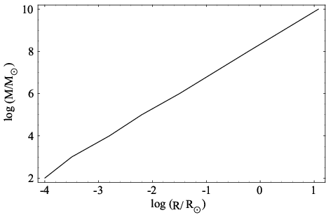
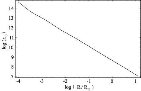
Figs. 2, 3 and 4 show the relations ” central density– mass” , ”central density–radius” and ”mass-radius” for the objects under consideration.

There are no solutions for greater masses.

In according to figure 4 the relation ”mass-radius” for these configuration is given by :

It is not clear, at present, whether the found solutions for the big masses make up a continuous class of solutions with the solutions for neutron stars and dwarfs or not. Besides, the above figures have not any extremes points. For this reason the figures do not give us direct evidences of the stability or instability of the objects under consideration.

The stability of the objects was argued first in paper [[Verozub 1996]] where the objects was considered as homogeneous. Following a classical method by [[Ledoux 1958]] and [[Cox 1980]] consider now the problem of the stability of the configurations more rigorously, without the assumption of homogeneity.

The complete energy of a spherically symmetric object of the mass $M$ and the radius $R$ can be written as follows

where $m$ is the mass of the matter inside the sphere of the radius $r,$ $u$ is the intrinsic energy, $\phi$ is the gravitational potential. The function $\mathcal{L}=u+\phi$ will be considered as the function of the variables $m$, $r(m)$ and $r^{\prime}(m)=dr/dm$. Consider the functional

on the set of all continuously differentiable function $r(m)$ with the boundary conditions $r(0)=0$, $r(M)=R$ and find at which conditions the first variation $\delta E$ is equal to zero and the second one is a positive at small isoentropic disturbances $r\longrightarrow r+\delta r$.

Since

the condition $\delta E=0$ yields the Lagrange equation and end condition.

The Lagrange equation

is given by

where $\left(\partial/\partial\rho\right)_{S}$ denotes the derivative at a constant value of the entropy $S$, $g=F/m_{p}$ and the force $F$ affecting the particle with mass $m_{p}$ is given by [[Verozub 1996]]

where $f=(r_{g}^{3}$ $+$ $r^{3})^{1/3}.$

Since the pressure is

the eq. (52) is the equation of hydrostatic equilibrium

When the Lagrange equation (51) is satisfied, the end condition can be obtained from the equality

where $\eta=\delta r$. Because of spherical symmetry we have $\eta\left(0\right)=0$, and $\eta\left(R\right)$ is an arbitrary magnitude, this equation leads to the following condition at the surface

The second variation $\delta^{2}E$ is of the form

where $2\Omega\left(\eta,\eta^{\prime}\right)=\mathcal{L}_{r^{\prime}r^{\prime}}\eta^{\prime 2}+2\mathcal{L}_{rr^{\prime}}\eta\eta^{\prime}+\mathcal{L}_{rr}\eta^{2}$ , $\eta^{\prime}=d\eta/dm$ and lower indices denote partial derivatives with respect to $r$ and $r^{\prime}$. The value of $\delta^{2}E$ is positive only, if the equation

has positive proper values $\sigma^{2}$. Boundary condition is given by

For the functions $\mathcal{L}_{r^{\prime}r^{\prime}}$, $\mathcal{L}_{rr^{\prime}}$ and $\mathcal{L}_{rr}$ we find

Using (54) and equality [[Cox 1980]],[[Shapiro 1983]]

where $\Gamma$ is the usual generalized adiabatic exponent [[Ledoux 1958]], that will be identified here with $\Gamma$ in the equation of state

($K$ is a constant), we obtain

Substituting these magnitudes in (59), we obtain following equation for dimensionless functions $\xi=\eta/r$:

where

The operator $\mathcal{Q}$ is selfconjugate in the Hilbert space. Its proper values $\sigma_{i}^{2}$ $\left(i=0,1\ldots\right)$ form an infinitely discrete sequence and are orthogonal with the weight $\rho r^{2}$ [[Cox 1980]]. Consequently, if $\xi_{k}$ are the proper function corresponding to the proper values $\sigma_{k}$, then

where $\xi^{\star}$ denotes the complex conjugate magnitude and

The numerator of eq. (67) consist of two integral. The first of them

$\geq 0$ and the second is given by

Since the magnitude $-g$ and the second term in eq. (69) are positive, at $\Gamma\geq 4/3$ the integral is positive. For that reason the proper values $\sigma^{2}>0$. Thus, at least at $\Gamma\geq 4/3,$ the configurations are stable.

References

• [Thirring 1961] Thirring, W.: 1961, Ann. Phys. 16, 96
• [Verozub 1991] Verozub, L.: 1991, Phys. Lett.A, 156, 404
• [Verozub 1996] Verozub, L.: 1996, Astr. Nachr., 317, 107
• [Verozub 1996] Verozub, L.: 1997 The Galactic Center, ASP Conference Series # 102, (Ed. R.Gredel), 357
• [Verozub 1997] Verozub, L.: 1997 The Identification of Dark Matter (Ed. N.Spooner), 195
• [Verozub 1999] Verozub, L.: 1999 Proceed. of ESO Workshop on Black Holes in binaries and Galactic Nuclei (In press)
• [Verozub and Kochetov 2000] Verozub, L. and Kochetov, A. : 2000, Grav. and Cosm., 6, 3(23), 246
• [Tolman 1969] Tolman, R.: 1969, Relativity Thermodynamics and Cosmology, Oxford
• [Harrison 1965] Harrison, B.K., Thorn K.S., Wakano M., Wheeler J.A.: 1965, Gravitational Theory and Gravitational Collapse. Univ.of Chicago Press. Chicago, Illinois
• [Ledoux 1958] Ledoux, P.: 1958, Stellar Stability, Handbuch der Physik, Band L1, 605
• [Cox 1980] Cox, J.: 1980, Theory of Stellar Pulsation, Princeton, New Jersey
• [Shapiro 1983] Shapiro, S.L., Teukolsky, S.A.: 1983, Black Holes, White Dwarfs and Neutron Stars. John Wiley & Sons
\addresses\rf
L.Verozub, Dept. of Physics and Astronomy, Kharkov National University, Kharkov, 61077, Ukraine,
e-mail: verozub@gravit.kharkov.ua \rfA.Kochetov, Dept. of Physics and Astronomy, Kharkov National University, Kharkov, 61077, Ukraine,
e-mail: alex@gravit.kharkov.ua