Characterizing 1-Dof Henneberg-I graphs with efficient configuration spaces

Heping Gao^* Meera Sitharam Note: University of Florida; Work supported in part by NSF Grants EIA 02-18435, CCF 04-04116, and a Research Gift from SolidWorks

Abstract

We define and study exact, efficient representations of realization spaces of a natural class of underconstrained 2D Euclidean Distance Constraint Systems(EDCS, Linkages, Frameworks) based on 1-degree-of-freedom(dof) Henneberg-I graphs. Each representation corresponds to a choice of parameters and yields a different parametrized configuration space. Our notion of efficiency is based on the algebraic complexities of sampling the configuration space and of obtaining a realization from the sample (parametrized) configuration. Significantly, we give purely combinatorial characterizations that capture (i) the class of graphs that have efficient configuration spaces and (ii) the possible choices of representation parameters that yield efficient configuration spaces for a given graph. Our results automatically yield an efficient algorithm for sampling realizations, without missing extreme or boundary realizations. In addition, our results formally show that our definition of efficient configuration space is robust and that our characterizations are tight. We choose the class of 1-dof Henneberg-I graphs in order to take the next step in a systematic and graded program of combinatorial characterizations of efficient configuration spaces. In particular, the results presented here are the first characterizations that go beyond graphs that have connected and convex configuration spaces.

Keywords: Underconstrained Geometric Constraint System, One Degree of Freedom(1-Dof), Henneberg-I Graph, Triangle-Decomposable Graph, Graph Minor, Graph Characterization, Configuration Space, Algebraic Complexity.

1 Introduction

A linkage is a graph $G=(V,E)$ with fixed length bars as the edges. Denote by $\delta:E\rightarrow\mathbb{R}^{1}$ the bar lengths. The degrees of freedom (dofs) of a linkage on the Euclidean plane refer to internal motions, after discounting Euclidean or rigid body motions that rotate or translate the entire linkage, preserving all pairwise distances. The problem of describing the plane realizations of one degree-of-freedom linkages or mechanisms has a long history.

A reasonable way to describe this space of realizations of a 1-dof linkage $(G,\delta)$ is to take a pair of vertices not connected by bars i.e, a non-edge $f$ , and ask for all the possible distance values $\delta^{*}$ that the non-edge $f$ can attain. This set of realizable distance values $\delta^{*}$ for the non-edge $f$ is called the configuration space of the linkage $(G,\delta)$ on $f$ , or parametrized by the distance $\delta^{*}(f)$ . This configuration space is a set of intervals on the real line.

For a well-known class of 1-dof linkages, we answer the following questions: How to describe the interval endpoints of such a configuration space? What is a reasonable and robust measure of complexity of this configuration space? Does the choice of non-edge $f$ influence this complexity? And using such a complexity measure, which graphs $G$ have configuration spaces of low complexity?

1.1 Summary of Contributions

Our class of 1-dof linkages is obtained from so-called Henneberg-I graphs, a natural subclass of Laman or minimally rigid graphs. These graphs can be constructed one vertex at a time, starting with a base edge $f$ . At each step of the construction a new vertex is added with edges between it and exactly 2 previously constructed vertices. See Figure 3. Delete the base edge $f$ , denote the resulting 1-dof Henneberg-I graph as $G=(V,E)$ , assign distances $\delta$ to the edges to obtain a 1-dof linkage $(G,\delta)$ .

Denote the configuration space of this linkage $(G,\delta)$ on $f$ as $\Phi_{f}(G,\delta)$ . As mentioned earlier, this is a set of intervals. Given an configuration $\delta^{*}$ in this set, a corresponding cartesian realization - which assigns the distance value $\delta^{*}$ to $f$ - can be computed using a ruler and compass: simply follow the partial order of the Henneberg construction, and realize each vertex as a point in $\mathbb{R}^{2}$ , by solving one quadratic equation in one variable at each step.

Algebraically, this is the solution of a triangularized system of quadratics the complexity of which is generally refered to as Quadratic or Radical Solvability.

More specifically, we answer the following questions.

(1)

What do the endpoints of the intervals in the set $\Phi_{f}(G,\delta)$ above correspond to? We show in Theorem 4.5 that they have a combinatorial meaning, in fact, they can be computed by realizing other linkages, called extreme linkages obtained from the graph $G$ and the non-edge $f$ .
(2)

For which $G$ and $f$ is the complexity of obtaining endpoints of the above intervals roughly the same as the ruler and compass realization complexity described above? More precisely, we use (1) and ask when are all the extreme linkages Quadratically solvable?

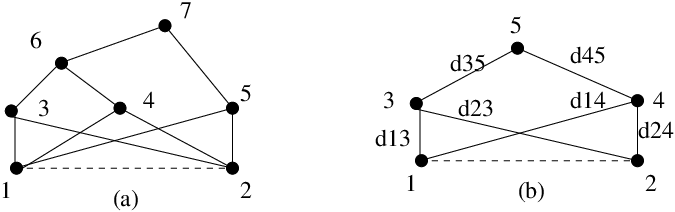
Figure 1: Figure (left) is a 1-Dof Henneberg-I graph whose configuration space on the base non-edge has interval endpoints that are not always quadratically solvable. Figure (right) on the other hand has quadratically solvable end points. For the edge distances show, the intervals are $[\frac{1}{8}\sqrt{6214-90\sqrt{17}\sqrt{209}},\frac{1}{8}\sqrt{6214+6\sqrt{17}\sqrt{209}}]$ and $[\frac{2}{5}\sqrt{565-360\sqrt{2}},\frac{2}{5}\sqrt{565+360\sqrt{2}}]$ .

Figure 1 shows two examples of graphs $G$ and non-edges $f$ : the interval endpoints are quadratically solvable for one of them, but not for the other.

In fact, we ask for which $G$ and $f$ , the extreme graphs have a graph property called Tree- or Triangle decomposability, which has been shown in [15] to be generically equivalent to Quadratic Solvability for planar graphs and the equivalence is strongly conjectured for all graphs. We say that such configuration spaces $\Phi_{f}(G,\delta)$ have low sampling complexity. We give in Theorem 4.7 a forbidden minor characterization of the property of low sampling complexity and in Observation 4.10 give a faster algorithm for finding the interval endpoints in $\Phi_{f}(G,\delta)$ than by realizing all the extreme graphs as per (1). We also show in Observations 4.11, 4.12 and 4.13 the tightness of this forbidden minor characterization by dropping various conditions and showing that no forbidden minor characterization will apply. Furthermore, in Theorem 4.14, we give an algorithmic characterization for a larger class of graphs.
(3)

Does the choice of the base non-edge $f$ matter ? A Henneberg-I graph could be constructible from different possible base edges and a 1-dof Henneberg-I graph could be obtained by deleting any one of them. Could these configuration spaces have different sampling complexities?

In Theorem 4.16 show that this cannot happen, thereby showing that our measure of sampling complexity for configuration spaces of 1-dof Henneberg-I linkages is robust.

1.2 Model of Computation

Our complexity measures are based on a model of computation that uses exact representation of numbers in any quadratic extension field of the rational numbers. In other words, we assume that all arithmetic operations, comparisons and extraction of square roots are constant time, exact operations. This model of computation is not as strong as the real RAM model that is normally used in computational geometry, that permits exact representation of arbitrary algebraic numbers [13]. Issues in exact geometric computation such as efficient and robust implementation of such a representation, for example using interval arithmetic, are beyond the scope of this manuscript.

1.3 Organization

In Section 2 we motivate and give a brief background for the overall program of investigation including various measures of efficiency of configuration spaces. The contributions of this manuscript are aligned with this program. Their novelty and technical significance is outlined in Section 3 together with related work. The theorems and proofs are presented in Section 4. We conclude with suggestions for future work in Section 5.

2 Overall Program and Motivation

We begin by clarifying and unifying terminology that arises in different communities that are interested in the same problems concerning configuration spaces of linkages. In geometric constraint solving terminology, a linkage is also called a Euclidean Distance Constraint System (EDCS) $(G,\delta)$ , i.e., is a graph $G=(V,E)$ together with an assignment of distances $\delta(e)$ , or distance intervals $[\delta^{l}(e),\delta^{r}(e)]$ to the edges $e\in E$ . A $d$ -dimensional realization is the assignment $p$ of points in $\mathbb{R}^{d}$ to the vertices in $V$ such that the distance equality (resp. inequality) constraints are satisfied: $\delta(u,v)=\|p(u)-p(v)\|$ (respectively $\delta^{l}(u,v)\leq\|p(u)-p(v)\|\leq\delta^{r}(u,v)$ ). Note: an EDCS with distance equality constraints, $(G,\delta)$ , was originally refered to as a framework in combinatorial rigidity terminology; more recently a framework $(G,p)$ includes a specific realization $p$ , and the distance assignment $\delta$ is read off from $p$ .

Note: We will use standard and well-known geometric constraint solving (and the corresponding combinatorial rigidity) terminology for which we refer the reader to, for example [16] [6] and [10]. In 2D, a graph $G=(V,E)$ is wellconstrained or minimally rigid if it satisfies the Laman conditions [12]; i.e., $|E|=2|V|-3$ and $|E_{s}|\leq 2|V_{s}|-3$ for all subgraphs $G_{s}=(V_{s},E_{s})$ of $G$ ; $G$ is underconstrained or independent and not rigid if we have $|E|<2|V|-3$ and $|E_{s}|\leq 2|V_{s}|-3$ for all subgraphs $G_{s}$ . A graph $G$ is overconstrained or dependent if there is a subgraph $G_{s}=(V_{s},E_{s})$ with $|E_{s}|>2|V_{s}|-3$ . $G$ is welloverconstrained or rigid if there exists a subset of its edges $E^{\prime}$ such that the graph $G^{\prime}=(V,E^{\prime})$ is wellconstrained or minimally rigid. A graph is flexible if it is not rigid.

One seeks efficient representations of the realization space of an EDCS. We define a representation to be (i) a choice of parameter set, specifically a choice of a set $F$ of non-edges of $G$ , and (ii) a set $\Phi_{F}^{d}(G,\delta)$ of possible distance values $\delta^{*}(f)$ that the non-edges in $f\in F\subseteq\overline{E}$ can take while ensuring existence of at least one $d$ -dimensional realization for the augmented EDCS: $(G\cup F,\delta(E),\delta^{*}(F))$ . Here $G\cup F$ refers to a graph $H:=(V,E\cup F)$ . In other words, the representations employ Cayley parameters: distances or sometimes squared distances corresponding to the non-edges in $F$ [4]. The set $\Phi_{F}^{d}(G,\delta)$ is the projection of the Cayley-Menger semi-algebraic set associated with $(G,\delta)$ on the Cayley parameters in $F$ . As mentioned earlier, we refer to the representation $\Phi_{F}^{d}(G,\delta)$ as the configuration space of the EDCS $(G,\delta)$ on the parameter set $F$ of non-edges of $G$ .

Describing and sampling the realization space of an EDCS is a difficult problem that arises in many classical areas of mathematics and theoretical computer science and has a wide variety of applications in computer aided design for mechanical engineering, robotics and molecular modeling. Especially for underconstrained (independent and not rigid) EDCS whose realizations have one or more internal degrees of freedom of motion, progress on this problem has been very limited.

Existing methods for sampling EDCS realization spaces often use Cartesian representations, factoring out the Euclidean group by arbitrarily “pinning” or “grounding” some of the points’ coordinate values. Even when the methods use internal representation parameters such as Cayley parameters (non-edges) or angles between unconstrained objects, the choice of these parameters is usually adhoc. While Euclidean motions are automatically factored out in the resulting parametrized configuration space, for most such parameter choices, the parametrized configuration space is still a topologically complex semi-algebraic set, often of reduced measure in high dimensions. The method of sampling is usually: “take a uniform grid sampling and throw away sample configurations that do not satisfy constraints.” Since even configuration spaces of full measure (representation with lowest possible number of parameters or dimensions) often have complex boundaries, this type of sampling method is likely to miss extreme and boundary configurations and is moreover computationally inefficient. To deal with this, numerical, iterative methods are generally used in case that the constraints are equalities, and in the case of inequalities, probabilistic “roadmaps” and other general collision avoidance methods are used. They are approximate methods that do not leverage exact descriptions of the configuration space.

Two related problems additionally occur in NMR molecular structure determination and wireless sensor network localization: completing a partially specified Euclidean Distance Matrix in a given dimension; and finding a Euclidean Distance Matrix in a given dimension that closely approximates a given Metric Matrix (representing pairwise distances in a metric space) [1, 3, 5]. The latter problem also arises in the study of algorithms for low distortion embedding of metric spaces into Euclidean spaces of fixed dimension [2]. Both of these problems can in fact directly be viewed as searching over a configuration space of an EDCS.

2.1 Exact, efficient configuration spaces

Motivated by these applications, our emphasis is on exact, efficient configuration spaces for underconstrained EDCS. First, an exact algebraic description, given by polynomial inequalities - whose coefficients are obtained after performing algebraic computations on the given EDCS - guarantees that boundary and extreme configurations are not missed during sampling, which is important for many applications.

Efficiency refers to several factors. We list four efficiency factors. The first factor is the sampling complexity: given the EDCS $(G,\delta)$ , (i) the complexity of computing (ia) the set of Cayley parameters or non-edges $F$ and (ib) the description of the configuration space $\Phi_{F}^{d}(G,\delta)$ as a semi-algebraic set, which includes the algebraic complexity of the coefficients in the polynomial inequalities that describe the semi-algebraic set, and (ii) the descriptive algebraic complexity, i.e., number, terms, degree etc of the polynomial inequalities that describe the semi-algebraic set. These together determine the complexity of sampling or walking through configurations in $\Phi_{F}^{d}(G,\delta)$ .

Concerning (i) it is important to note that most choices of Cayley parameters (non-edges) to represent the realization space of $(G,\delta)$ give inefficient descriptions of the resulting parametrized configuration space. Hence a strong emphasis needs to be placed on a systematic, combinatorial choice of the Cayley parameters that guarantee a configuration space with all the efficiency requirements listed here. Further, we are interested in combinatorially characterizing for which graphs $G$ such a choice even exists.

The second efficiency factor is the realization complexity. Note that the price we pay for insisting on exact and efficient configuration spaces is that the map from the traditional Cartesian realization space to the parametrized configuration space is many-one. I.e, each parametrized configuration could correspond to many (but at least one) Cartesian realizations.

However, we circumvent this difficulty by defining and studying realization complexity as one of the requirements on efficient configuration spaces i.e., we take into account that the realization step typically follows the sampling step, and ensure that one or all of the corresponding Cartesian realizations can be obtained efficiently from a parametrized sample configuration.

A third efficiency factor is generic completeness, i.e, we would like each configuration in our parametrized configuration space to generically correspond to at most finitely many Cartesian realizations and moreover, we would like the configuration space to be of full-measure, i.e, use exactly as many parameters or dimensions as the internal degrees of freedom of $G$ . Combinatorially this means that the graph $G\cup F$ is well-constrained or minimally rigid in combinatorial rigidity terminology.

A fourth important efficiency factor is topological complexity for example, connectedness or number of connected components and geometric complexity for example convexity; however, for this manuscript, these factors are subsumed in the sampling complexity since configuration space of this manuscript is a 1-parameter space.

In [8] and [17] a series of exact combinatorial characterizations are given for connected, convex and complete configuration spaces of low sampling and realization complexity for general 2D and 3D EDCSs (including distance inequalities), and a somewhat weaker characterization is given for arbitrary dimensional EDCSs.

2.2 Combinatorial Characterization

Combinatorial characterizations of generic properties of EDCS are the cornerstone of combinatorial rigidity theory. In practice they crucial for tractable and efficient geometric constraint solving, since they are used to analyze and decompose the underlying algebraic system. So far such characterizations have been used primarily for broad classifications into well- over- under- constrained, detecting dependent constraints in overconstrained systems and finding completions for underconstrained systems. Such combinatorial characterizations have been missing in the finer classification of underconstrained systems according to the efficiency or complexity of their configuration space. This however is a crucial step in efficiently decomposing and analyzing underconstrained systems. Our emphasis in this respect is the surprising fact that there is a clean combinatorial characterization at all of the algebraic complexity of configuration spaces.

The PhD thesis [8] formulates the concept of efficient configuration space description for underconstrained EDCS, by emphasizing the systematic choice of parameters that yield efficient representations of the realization space, setting the stage for a mostly combinatorial, and complexity-graded program of investigation. An initial sketch of this program was presented in [9]; a comprehensive list of theoretical results and applications to date can be found in the PhD thesis [8]. In this manuscript, we take the first step in one of two natural directions to move beyond [17] which characterizes graphs whose EDCS always admit convex and/or connected 2D configuration spaces. One possible extension direction is to ask which graphs always admit 2D configuration spaces with at most 2 connected components. Results in this direction can be found in [8]. A second possible direction, is to take the simplest natural class of graphs with 1-dof (generic mechanisms with 1-degree-of-freedom) that do not have connected configuration spaces, and combinatorially classify them based on their sampling complexity. This is the direction we take here.

3 Novelty and Related Work

Our results give a practically meaningful, and mathematically robust definition of efficient configuration spaces for a natural class of 1-dof linkages or EDCS, based on algebraic complexity of sampling and realization. Significantly, we give purely combinatorial, tight characterizations that capture (i) the class of EDCS that have such configuration spaces and (ii) the possible choices of parameters that yield such configuration spaces.

To the best of our knowledge, the only known result in this area that has a similar flavor of combinatorially capturing algebraic complexity is the result of [15] that relates quadratic solvability and Tree- or Triangle- decomposability for planar graphs.

Concerning the use of Cayley parameters or non-edges for parametrizing the configuration space: the papers [11], [16] and [19] study how to obtain “completions” of underconstrained graphs $G$ , i.e, a set of non-edges $F$ whose addition makes $G$ well-constrained or minimally rigid. All are motivated by the need to efficiently obtain realizations of underconstrained EDCS. In particular [11] also guarantees that the completion ensures Tree- or Triangle- decomposability, thereby ensuring low realization complexity.

However, they do not even attempt to address the question of how to find realizable distance values for the completion edges. Nor do they concern themselves with the geometric, topological or algebraic complexity of the set of distance values that these completion non-edges can take, nor the complexity of obtaining a description of this configuration space, given the EDCS $(G,\delta)$ and the non-edges $F$ , nor a combinatorial characterization of graphs for which this sampling complexity is low. The latter factors however are crucial for tractably analyzing and decomposing underconstrained systems and for sampling their configuration spaces in order to obtain the corresponding realizations. The problem has generally been considered too messy, and there has been no systematic, formal program to study this problem.

On the other hand, [14] gives a collection of useful observations and heuristics for computing the interval endpoints in the configuration space descriptions of certain graphs that arise in real CAD applications.

4 Results

4.1 Definition and basic properties of Simple 1-dof Henneberg-I graphs

As mentioned in the Introduction, Henneberg-I graphs can be constructed one vertex at a time, starting with a base edge. At each step $k$ of the construction a new vertex $v_{k}$ is added with edges to exactly 2 previously constructed vertices $u,w$ , called the base pair of vertices at step $k$ . We denote this by $v_{k}\triangleleft u,w$ . In fact, a Henneberg-I construction $c$ is actually a partial order that is completely specified by the base edge $f$ , although we loosely use the phrase construction sequence to refer to this partial order. See Figure 3. We consider this class because it is the smallest natural class that contains 2-trees (sometimes called graphs of tree-width 2) which figure prominently in the combinatorial characterizations of convex and connected configuration spaces for 2D EDCS in [8, 17], as mentioned in Section 2. In other words, Henneberg-I graphs are the simplest generalization of 2-trees which do not have convex or connected configuration spaces. Henneberg-I graphs are a natural subclass of Laman or minimally rigid graphs, and also of another common class of graphs called Tree- or Triangle- decomposable graphs[6], that are conjectured to be exactly equivalent to quadratically solvable graphs, a conjecture that has been proven for planar [15].

Refer to caption — Figure 2: Tree-Decomposable Graph: a graph $G$ is Tree-Decomposable if it can be divided into three Tree-Decomposable subgraphs $G_{1}$ , $G_{2}$ and $G_{3}$ such that $G=G_{1}\cup G_{2}\cup G_{3}$ , $G_{1}\cap G_{2}=(\{v_{3}\},\emptyset)$ , $G_{2}\cap G_{3}=(\{v_{2}\},\emptyset)$ and $G_{1}\cap G_{3}=(\{v_{1}\},\emptyset)$ where $v_{1}$ , $v_{2}$ and $v_{3}$ are three different vertices; as base cases, a pure edge and a triangle are defined to be Tree-Decomposable.

A graph $G$ is Triangle-Decomposable or Tree-Decomposable, if:

•

it is a pure edge or a triangle; or
•

it can be divided into three Triangle-Decomposable subgraphs $G_{1}$ , $G_{2}$ and $G_{3}$ such that $G=G_{1}\cup G_{2}\cup G_{3}$ , $G_{1}\cap G_{2}=(\{v_{3}\},\emptyset)$ , $G_{2}\cap G_{3}=(\{v_{2}\},\emptyset)$ and $G_{1}\cap G_{3}=(\{v_{1}\},\emptyset)$ where $v_{1}$ , $v_{2}$ and $v_{3}$ are three different vertices (refer to Figure 2)[6].

We also say $G_{1}$ , $G_{2}$ and $G_{3}$ are clusters and $v_{1}$ , $v_{2}$ and $v_{3}$ are shared vertices.

A generalization of the results presented here from Henneberg-1 graphs to the larger class of Tree- or Triangle-decomposable graphs appears in [8] and [18].

A Simple 1-dof Henneberg-I graph $G$ is obtained by removing a base edge $f$ from a Henneberg-I graph (note that there can be more than 1 possible base edge for a given Henneberg-I graph, refer to Figure 15). Such an edge $f$ is called a base non-edge of $G$ . The EDCSs $(G,\delta)$ based on such graphs generically have one internal degree of freedom and hence a complete, 1-parameter configuration space.

The notion of an extreme graph of a Simple 1-dof Henneberg-I graph $G$ with base non-edge $f$ will be used prominently in our results. The $k^{th}$ extreme graph $X_{k}$ based on $G$ and $f$ is obtained from $G$ by adding a new edge $(u,w)$ between the base pair of vertices $u$ and $w$ of the $k^{th}$ Henneberg construction step $v_{k}\triangleleft u,w$ , provided $u,w$ do not belong to any well-constrained subgraph of $G$ (otherwise, the $k^{th}$ extreme graph is overconstrained and irrelevant - depending on the context it could be left undefined). For the linkage or EDCS $(G,\delta)$ and the non-edge $f$ , the $k^{th}$ extreme linkage or EDCS $X_{k,j},j=1,2$ is $(X_{k},\delta^{j})$ , where the $j=1,2$ represents two possible extensions of $\delta$ to the new edge $(u,w)$ : $\delta^{1}(u,w):=\delta(u,v_{k})+\delta(v_{k},w)$ , and $\delta^{2}(u,w):=|\delta(u,v_{k})-\delta(v_{k},w)|$ .

Next we prove a series of facts giving basic properties of 1-dof Henneberg-I graphs that will be used in our main results and are additionally of independent interest since these graphs are commonly occuring.

Fact 4.1

No subgraph of a Simple 1-dof Henneberg-I graph is overconstrained (i.e., it is independent). A subgraph $G^{\prime}$ of a Simple 1-dof Henneberg-I graph is wellconstrained (minimally rigid) if and only if $G^{\prime}$ is a Henneberg-I graph.

Proof First we prove that no subgraph of a Simple 1-dof Henneberg-I graph is overconstrained by showing that such a graph $G$ satisfies the Laman sparsity or independence condition [12]: i.e, the number of edges of any subgraph is at most twice the number of vertices minus 3. First, we consider the list of vertices of $G$ obtained from a Henneberg-I construction sequence $s$ for $G$ with base non-edge $f$ . That is, $s$ is a Henneberg-I construction sequence for $G\cup f$ , starting from $f$ . We start the list with the two vertices of $f$ , (any relative ordering of these two vertices is fine). Then, we add all the other vertices to the list one by one strictly following the construction sequence $s$ . One property of Henneberg-I sequences is that any vertex not in the first two slots of the list is adjacent to exactly two vertices which are before it in the list. For any subgraph $G^{\prime}$ , we can get a new list by extracting the sublist corresponding to the vertices of $G^{\prime}$ from this list. In this sublist, any vertex is adjacent to at most two vertices which are before it. Therefore, if the number of the vertices of $G^{\prime}$ is $n$ , the number of the edges of $G^{\prime}$ will not exceed $1+2(n-2)=2n-3$ , thus ensuring the Laman sparsity or independence condition.

Then we prove that a subgraph $G^{\prime}$ of a Simple 1-dof Henneberg-I graph is wellconstrained (minimally rigid) if and only if $G^{\prime}$ is a Henneberg-I graph. One direction is clear since any Henneberg-I graph is wellconstrained.

For the other direction, by Laman’s theorem [12], the number of edge of $G^{\prime}$ has to be $2n-3$ if $G^{\prime}$ is wellconstrained. We have just proved that the number of edge in $G^{\prime}$ does not exceed $2n-3$ . For the equality to be true, there must be one edge between the first two vertices in the sublist and any vertex in the third or higher slot in the sublist must be adjacent to exactly two vertices before it in the sublist. By the definition of Henneberg-I graph, this implies $G^{\prime}$ has to be a Henneberg-I graph. $\Box$

Fact 4.2

Given a Simple 1-dof Henneberg-I graph $G$ with base non-edge $f=(v_{1},v_{2})$ , no wellconstrained subgraph $G^{\prime}$ of $G$ can contain both $v_{1}$ and $v_{2}$ .

Proof The contrapositive follows from Fact 4.1 and its proof. That lemma states that $G^{\prime}$ must be a Henneberg-I graph if it is wellconstrained and its proof points out that if $G^{\prime}$ contains $v_{1}$ and $v_{2}$ , there must be an edge the first two vertices in the sublist which are $v_{1}$ and $v_{2}$ here. This contradicts $(v_{1},v_{2})$ being the base non-edge of $G$ . $\Box$

Fact 4.3

Take a Simple 1-dof Henneberg-I graph $G=(V,E)$ with a base non-edge $(v_{1},v_{2})$ and corresponding Henneberg-I construction sequence $(v_{3}\triangleleft(u_{3},w_{3}),\cdots,v_{n}\triangleleft(u_{n},w_{n})$ where $n=|V|$ . Then

1.

for any $m$ , the extreme graph corresponding to $v_{m}\triangleleft(u_{m},w_{m})$ , i.e., the graph obtained by adding the edge $(u_{m},w_{m})$ is wellconstrained if and only if there is no wellconstrained subgraph in $G$ that contains both $u_{m}$ and $w_{m}$ .
2.

If there exists a subgraph $G^{\prime}$ containing $u_{m}$ and $w_{m}$ that is wellconstrained, then we can say the following. Taking $G_{m-1}$ to be the graph constructed before $v_{m}$ and let $G_{m}=G_{m-1}\cup v_{m}$ Now for any distance assignment $\delta$ we have $\Phi_{f}^{2}(G_{m},\delta)=\Phi_{f}^{2}(G_{m-1},\delta)$ or $\Phi_{f}^{2}(G_{m},\delta)=\emptyset$ .

Proof We first prove (1). If there is a wellconstrained subgraph $G^{\prime}$ containing both $u_{m}$ and $w_{m}$ , then $G^{\prime}\cup(u_{m},w_{m})$ will be overconstrained. This proves one direction. For the other direction, if there is no wellconstrained subgraph $G^{\prime}$ containing both $u_{m}$ and $w_{m}$ , $G\cup(u_{m},w_{m})$ will not have any overconstrained subgraphs; and since $G$ is 1-dof, $G\cup(u_{m},w_{m})$ would be wellconstrained (both by Laman’s theorem [12]). This proves the other direction.

For (2), by Fact 4.1, $G^{\prime}$ is a Henneberg-I graph with a base edge, say $(v_{i},v_{j})$ . If we remove all the vertices of $G^{\prime}$ other than $v_{i}$ and $v_{j}$ . we can get a subgraph $G^{*}$ . Now $G$ is a 2-sum of $G^{\prime}$ and $G^{*}$ , i.e $G^{\prime}$ and $G^{*}$ hinged together at an edge, so for any $\delta$ $(G,\delta)$ has a realization if and only if $(G^{*},\delta)$ has a realization and $(G^{\prime},\delta)$ has realization. Furthermore, either $\Phi_{f}^{2}(G,\delta)=\Phi_{f}^{2}(G^{*},\delta)$ or $\Phi_{f}^{2}(G,\delta)=\emptyset$ . Note this property holds if we add more vertices to $G^{\prime}$ by Henneberg-I steps. Thus, we have $\Phi_{f}^{2}(G_{m},\delta)=\Phi_{f}^{2}(G_{m-1},\delta)$ or $\Phi_{f}^{2}(G_{m},\delta)=\emptyset$ . $\Box$

4.2 Characterizing Simple 1-dof Henneberg-I graphs with efficient configuration spaces

For Simple 1-dof Henneberg-I graphs $G$ , a natural choice of configuration space parameter is its base non-edge. We simply adopt this choice of parameter since it guarantees a complete configuration space of low realization complexity, i.e., quadratically solvable in time linear in $|V|$ , as mentioned in the introduction. Unlike general Tree- or Triangle- decomposable graphs, since Henneberg-I graphs have a single base edge, they are some times called ruler and compass constructible or RCC graphs).

Note that this realization process could lead to an exponential combinatorial explosion because there are 2 possible orientations for each point $p(v)$ and only one of them may successfully lead to a realization of the entire EDCS. However, we will show in Observation 4.6 that we can circumvent this problem by encoding along with each parametrized configuration $\delta^{*}(f)$ , one (or all) of the orientations $\sigma$ (defined below) of its corresponding realizations. Thus the realization complexity is essentially linear in $|V|$ .

With this in mind, we only need to characterize which Simple 1-dof Henneberg-I graphs $G$ have low sampling complexity for their configuration space on the base non-edge $f$ . Specifically, this is a 1-parameter configuration space, and hence it consists of a union of intervals. The sampling complexity is thus the complexity of determining the endpoints of these intervals, starting with $(G,\delta)$ as input.

In order to quantify and define low sampling complexity we prove a crucial result Theorem 4.5 that gives a combinatorial meaning to the endpoints of the intervals in the configuration space $\Phi_{f}^{2}(G,\delta)$ . The theorem relies on a technical Lemma 4.4 that gives combinatorial description of the configuration space. The proof requires basic algebra and real analysis.

4.2.1 Combinatorial meaning of configuration space boundary

We first formally define the orientation of a realization of a Henneberg-I graph. As mentioned above, given an EDCS $(H,\delta)$ where $H$ is a Henneberg-I graph with base edge $f$ , for each Henneberg-I step $v_{k}\triangleleft(u_{k},w_{k})$ , if the coordinates for the point realizations $p(u_{k})$ and $p(w_{j})$ are known and the values $\delta(v_{k},u_{k})$ and $\delta(v_{k},w_{k})$ are also known, the posssible coordinates for the point $p(v_{k})$ can be determined by a corresponding simple ruler and compass algebraic construction (solving a quadratic equation in 1 variable). If the triangle is not a trivial one (three vertices are not collinear), there are two choices for the coordinates of $p(v_{k})$ . We say each of these choices is an orientation $\sigma_{k}$ for the Henneberg-I step $k$ . If we specify an orientation for each Henneberg-I step in a construction sequence (partial order) of $H$ from $f$ , yielding a corresponding sequence (partial order) $\sigma$ , we say that a realization of $(H,\delta)$ has an orientation $(\sigma,f)$ .

In fact, observe that this is a 1-1 correspondence provided $\delta$ assigns distinct distances to the edges of $H$ . I.e, for any such $\delta$ , there exists at most one 2D realization $p$ of $(H,\delta)$ , when an orientation $(\sigma,f)$ is specified. The coordinates of $p(v_{k})$ are not unique only if at the $k^{th}$ step of the construction sequence $c$ the vertex $v_{k}$ is constructed from vertices $u_{K}$ and $w_{k}$ for which $p(u_{k})$ and $p(w_{k})$ are coincident and $\delta(v_{k},u_{k})$ is equal to $\delta(v_{k},w_{k})$ . See Figure 5.

Now consider an EDCS $(G,\delta)$ where $G$ is a Simple 1-dof Henneberg-I graph with base non-edge $f,$ and assume $\delta$ assigns distinct values. For any such $\delta$ and distance assignment $\delta^{*}(f)$ distinct from the values assigned by $\delta$ , an orientation $(\sigma,f)$ (and realization) for $(G\cup f,\delta,\delta^{*})$ gives a corresponding orientation (and realization) for $(G,\delta)$ . At any construction step, we can regard $\delta^{*}(u,w)$ for the base pair of vertices as a function of $\delta^{*}(f)$ . The next lemma analyzes this function to give a combinatorial description for $\Phi_{f}^{2}(G,\delta)$ .

Lemma 4.4

Given an EDCS $(G,\delta)$ where $G$ is a Simple 1-dof Henneberg-I graph with base non-edge $f=(v_{1},v_{2})$ , if (1) for all Henneberg-1 steps $v\triangleleft(u,w)$ in the construction sequence starting from $f$ , the two edge distances $\delta(v,u)$ and $\delta(v,w)$ are distinct and (2) an orientation $\sigma$ is specified for the Henneberg-I construction sequence starting from $f$ , then the following hold:

1.

$\Phi_{f}^{2}(G,\delta)$ is a set of closed real intervals or empty;
2.

For any interval endpoint $\delta^{*}(f)$ in $\Phi_{f}^{2}(G,\delta)$ , there is a unique realization for $(G\cup f,\delta,\delta^{*}(f))$ with the orientation $\sigma$ and there exists a Henneberg-I step $v\triangleleft(u,w)$ such that the three vertices $v$ , $u$ and $w$ are collinear in this unique realization;
3.

For any pair of vertices $(u,w)$ and any realization $p$ of $(G\cup f),\delta,\delta^{*}(f))$ the distance $\delta^{*}_{p}(u,w)$ is a continuous function of $\delta^{*}(f)$ on each closed interval of $\Phi_{f}^{2}(G,\delta)$ . Furthermore, for any vertex, $v$ , the coordinates of the point $p(v)$ are continuous functions of $\delta^{*}(f)$ on each closed interval of $\Phi_{f}^{2}$ , if we pin the coordinates of $p(v_{1})$ to be $(0,0)$ and the $y$ -coordinate of $p(v_{2})$ to be 0.

The proof of this lemma involves basic algebra and real analysis. The idea is to do a ruler-and-compass realization sequence that follows a Henneberg-I construction sequence and check how each Henneberg-I step will change the configuration space on the base non-edge. In the following, we will loosely use “Henneberg construction sequence” also to refer to the corresponding ruler-and-compass realization sequence.

Proof [Lemma 4.4] We prove by induction on the length of the given Henneberg-I construction sequence starting from $f$ .

In the base case, the length of the given Henneberg-I construction sequence is 1. Suppose $v_{3}$ is the only other vertex. By the triangle inequality, we know $\Phi_{f}^{2}(G,\delta)$ is $[|\delta(v_{3},v_{1})-\delta(v_{3},v_{2})|,|\delta(v_{3},v_{1})+\delta(v_{3},v_{2})|]$ , so (1) and (2) are satisfied. For (3), we only need to consider whether the coordinates of $p(v_{3})$ which we denote as $(x_{v_{3}},y_{v_{3}})$ are a continuous function of $\delta^{*}(f)$ . Denote $R_{1}=\delta(v_{1},v_{3})$ , $R_{2}=\delta(v_{3},v_{2})$ and $R_{3}=\delta^{*}(v_{1},v_{2})=\delta^{*}(f)$ . We can compute

x_{v_{3}}=\frac{R_{1}^{2}+R_{3}^{2}-R_{2}^{2}}{2R_{3}}

(1)

y_{v_{3}}=\frac{\sqrt{(R_{1}+R_{2}+R_{3})(R_{1}+R_{2}-R_{3})(R_{1}-R_{2}+R_{3})(-R_{1}+R_{2}+R_{3})}}{2R_{3}}.

(2)

Note that since $R_{3}$ is not 0, both $x_{v_{3}}$ and $y_{v_{3}}$ are continuous fuctions of $R_{3}$ , which is our $\delta^{*}(f)$ now.

By induction hypothesis, we assume that (1), (2) and (3) hold for a Simple 1-dof Henneberg-I graph $G_{k-1}=(V,E)$ with base non-edge $f$ with less than $k$ Henneberg steps. Suppose we get a new graph $G_{k}$ by one more Henneberg-I step $v_{k}\triangleleft(u_{k},w_{k})$ with base vertices $u_{k},w_{k}$ in $G_{k-1}$ . I.e., $G_{k}=(V\cup v_{k},E\cup(v_{k},u_{k})\cup(v_{k},w_{k}))$ . We will prove (1), (2) and (3) hold for $G_{k}$ .

According to the Statement (3) of the induction hypothesis, in the realization $p$ of $G_{k-1}$ with a fixed orientation $\sigma$ , for any pair of vertices $(u,w)$ of $G_{k-1}$ , the distance value $\delta^{*}_{p}(u,w)$ is a continuous function, say $p_{u,w}$ , of $\delta^{*}(f)$ . We extend the realization $p$ to the newly added vertex $v_{k}$ . Now the edges $(v_{k},u_{k})$ and $(v_{k},w_{k})$ will restrict $\delta^{*}_{p}(u_{k},w_{k})$ to be in $[min,max]$ where $min=|\delta(v_{k},u_{k})-\delta(v_{k},w_{k})|$ and $max=\delta(v_{k},u_{k})+\delta(v_{k},w_{k})$ . This restriction will create new candidate interval endpoints in $\Phi_{f}^{2}(G_{k},\delta)$ , namely $p_{u_{k},w_{k}}^{-1}(\delta^{*}_{p}(u,v)),y\in[|\delta(v_{k},u_{k})-\delta(v_{k},w_{k})|,|\delta(v_{k},u_{k})+\delta(v_{k},w_{k})]$ , as is shown in Figure 6. Since these new candidate interval endpoints in $\Phi_{f}(G_{k},\delta)$ correspond to the realization in which $p(u_{k})$ , $p(v_{k})$ and $p(u_{k})$ are collinear, (1) and (2) are also true for graph $G_{k}$ .

To show the induction step for (3), take any non-edge $(u,w)$ . We have:

\delta_{p}^{*}(u,w)=\sqrt{(x_{u}-x_{w})^{2}+(y_{u}-y_{w})^{2}}

(3)

If $u\not=v_{k}$ and $w\not=v_{k}$ , $\delta^{*}_{p}(u,w)$ is clearly a continuous function of $\delta^{*}(f)$ , so we only need consider the case that either $u=v_{k}$ or $w=v_{k}$ .

For convenience, first rotate and translate the coordinate system so that in the triangle $\triangle(u_{k},w_{k},v_{k})$ , $u_{k}$ is at the origin and $\vec{u_{k},w_{k}}$ is the $x$ -axis. Without loss of generality, let $p(v_{k})$ be located above the line joining $p(u_{k})$ and $p(w_{k})$ , by the given orientation $\sigma$ in the statement of the Lemma. Denote $R_{1}=\delta(v_{k},u_{k})$ , $R_{2}=\delta(v_{k},w_{k})$ and $R_{3}=\delta_{p}^{*}(u_{k},w_{k})$ . Then,

x_{v_{k}}=\frac{R_{1}^{2}+R_{3}^{2}-R_{2}^{2}}{2R_{3}}

(4)

and

y_{v_{k}}=\frac{\sqrt{(R_{1}+R_{2}+R_{3})(R_{1}+R_{2}-R_{3})(R_{1}-R_{2}+R_{3})(-R_{1}+R_{2}+R_{3})}}{2R_{3}}.

(5)

Since we have restricted $R_{1}\not=R_{2}$ , we have $R_{3}>0$ . Consider the rotation and translation that now put the point $p(v_{1})$ at the origin and $p(v_{2})$ on the $x$ -axis as in the statement of the Lemma. Denote the rotation angle as $\beta$ . Then we have:

\cos\beta=\frac{x_{w_{k}}-x_{u_{k}}}{R_{3}}

(6)

\sin\beta==\frac{y_{w_{k}}-y_{u_{k}}}{R_{3}}

(7)

So we can get the transformed coordinates of $p(v_{k})$ :

x_{v_{k}}^{*}=x_{u_{k}}+x_{w_{k}}*\cos\beta+y_{k}*\sin\beta

(8)

y_{v_{k}}^{*}=y_{u_{k}}+x_{w_{k}}*\sin\beta+y_{k}*\cos\beta

(9)

$x_{v_{k}}$ and $y_{v_{k}}$ is a function of $x_{u_{k}}$ , $y_{u_{k}}$ , $x_{w_{k}}$ and $y_{w_{k}}$ , so for any value $\delta^{*}(f)$ over a closed interval, the coordinates $p(v_{k})$ can be expressed as a function of $\delta^{*}(f)$ using radicals. So, $\delta(u,w)$ in equation 3 is a continuous function of $\delta^{*}(f)$ even if $u=v_{k}$ or $w=v_{k}$ and this proves the induction step of Statement (3) of the Lemma 4.4 for graph $G_{k}$ . $\Box$

Remark. In Lemma 4.4, we require that the two distances $\delta(v_{k},u_{k})$ and $\delta(v_{k},w_{k})$ are not equal for the $k^{th}$ Henneberg-I step $v_{k}\triangleleft(u_{k},w_{k})$ . This requirement guarantees that the two points $p(u_{k})$ and $p(w_{k})$ in a realization $p$ for $(G_{k-1},\delta)$ are not coincident, whereby the quantity $R_{3}>0$ and thus we can use a continuity argument.

Now we can state the theorem that interests a combinatorial meaning to the configuration space of a Simple 1-dof Henneberg-I graph using the notion of extreme graphs defined earlier.

Theorem 4.5

Given an EDCS $(G,\delta)$ where $G$ is a Simple 1-dof Henneberg graph with a base non-edge $f$ , the endpoints of the intervals in the configuration space $\Phi_{f}^{2}(G,\delta)$ are contained in the set: ${\cal E}(G,\delta):=\bigcup\limits_{\sigma}\bigcup\limits_{1\leq k\leq|V|-2}\bigcup\limits_{1\leq j\leq 2}\{\delta^{X_{k,j}^{1,\sigma}}(f),\delta^{X_{k,j}^{2,\sigma}}(f),\ldots\}$ ;
where $\delta^{X_{k,j}^{m,\sigma}}(f)$ denotes the length or distance value of $f$ in the $m^{th}$ realization $p_{m}$ with orientation sequence $\sigma$ of the $k^{th}$ extreme EDCS $X_{k,j}$ determined by the pair $(G,f)$ .

Fact 4.3(1) guarantees that the graph corresponding to this extreme EDCS is wellconstrained provided the two vertices incident on the new edge were not previously in a wellconstrained subgraph. If they were in a wellconstrained subgraph, then the corresponding two EDCSs $X_{k,1}$ and $X_{k,2}$ can be left undefined, and the corresponding interval endpoints do not appear in ${\cal E}(G,\delta)$ by Fact 4.3(2).

Proof The proof directly follows from Statement (2) of Lemma 4.4 (2). $\Box$

Observation 4.6

Theorem 4.5 implies linear realization complexity of the configuration space $\phi_{f}^{2}(G,\delta)$ : for each candidate orientation sequence $\sigma$ , we can read off a set of intervals ${\cal I}_{\sigma}$ from the description ${\cal E}(G,\delta)$ as in Theorem 4.5, such that a configuration $\delta^{*}(f)\in{\cal I}_{\sigma}$ is guaranteed to correspond to a realization with the orientation $\sigma$ . Knowing a realizable orientation $\sigma$ for the configuration $\delta^{*}(f)$ eliminates the combinatorial explosion during a linear time ruler-and-compass realization of $(G\cup f,\delta,\delta^{*})$ .

Proof By Theorem 4.5 the endpoints of $\Phi_{f}^{2}(G,\delta)$ form a subset of the candidate set ${\cal E}(G,\delta)$ , which we view as a union over candidate sets for each orientation $\sigma$ : $\bigcup\limits_{\sigma}{\cal E}_{\sigma}(G,\delta)$ . While every such candidate configuration $\delta^{*}(f)$ is a configuration of an extreme EDCS of $G$ , not every candidate configuration is actually an interval endpoint for $\Phi_{f}^{2}(G,\delta)$ , nor even an endpoint of the set of intervals ${\cal I}_{\sigma}$ required in the statement of the Observation. To see this, recall the proof for Lemma 4.4(Figure 6); let $v_{k}$ be the vertex constructed in the $k^{th}$ step of the Henneberg construction of $G\cup f$ starting from $f$ , and let $u_{k}$ and $w_{k}$ be the base vertices of this step. Consider the continuous function $p_{u_{k},w_{k}}$ in the variable $\delta^{*}(f)$ which gives the distance between $u_{k}$ and $w_{k}$ in a particular realization $p$ with orientation $\sigma$ ; i.e, the value of this continuous function $p_{u_{k},v_{k}}$ evaluated at $\delta^{*}(f)$ is the distance $\delta^{*}_{p}(u_{k},w_{k})$ . Figure 7 shows that based on this continuous function, the 2 distance values $min=|\delta(v_{(}k),u_{k})-\delta(v_{(}k),w_{k})|$ and $max=|\delta(v_{(}k),u_{k})-\delta(v_{k},w_{k})|$ , all the following four cases are possible for a candidate configuration $\delta^{X_{k,j}^{m,\sigma}}(f)$ : neither the left nor the right neighborhood falls into $\Phi_{f}^{2}(G,\delta)$ ; both the left and the right neighborhood fall into $\Phi_{f}^{2}(G,\delta)$ ; the left falls into $\Phi_{f}^{2}(G,\delta)$ but the right does not; and symmetrically the right falls into $\Phi_{f}^{2}(G,\delta)$ but the left does not. In the first case, the candidate configuration is an isolated point in ${\cal I}_{\sigma}$ . In the second, it is not an endpoint of any interval in ${\cal I}_{\sigma}$ . In the third and the fourth cases, it is actually an endpoint of an interval in ${\cal I}_{\sigma}$ .

In other words, in order to produce such a set of intervals ${\cal I}_{\sigma}$ from the candidate configurations ${\cal E}_{\sigma}(G,\delta)$ , we need to check whether the left and/or right neighborhood of each such candidate configuration also belongs to $\Phi_{f}^{2}(G,\delta)$ , i.e, whether it has a realization. To find out which of the above 4 cases applies, one can check if there is any realization with orientation $\sigma$ , for values of $\delta^{*}(f)$ that are to the left (resp. right) of $\delta^{X_{k,j}^{m,\sigma}}(f)$ , but before the candidate configuration in ${\cal E}_{\sigma}(G,\delta)$ that is immediately preceding (resp. immediately succeeding) $\delta^{X_{k,j}^{m,\sigma}}(f)$ . This is straightforward after sorting the set ${\cal E}_{\sigma}(G,\delta)$ . Since the orientation is fixed, checking if such realizations exist can be done in linear time with a ruler and compass construction. $\Box$

Based on such a description of the configuration space $\Phi_{f}^{2}(G,\delta)$ , we say it has low sampling complexity if all of the extreme EDCS are Tree- or Triangle-decomposable, which ensures that the interval endpoints $\delta^{X_{i,j}^{k}}(f)$ in the above theorem can be computed essentially using a sequence of solving one quadratic equation at a time. This ensures linear complexity in $|V|$ It has additionally been conjectured these graphs exactly capture Quadratic Solvability and the conjecture has been proven for planar graphs [15].

4.2.2 Forbidden minor characterization for 1-path triangle-free Simple 1-dof Henneberg-I graphs

The next theorem gives a surprising and exact forbidden-minor characterization of a large class of Simple 1-dof Henneberg-I graphs $G$ with base non-edge $f$ such that for all distance assignments $\delta$ , the EDCS $(G,\delta)$ , the a configuration space $\Phi_{f}^{2}(G,\delta)$ has low sampling complexity. In other words, all the extreme graphs obtained from $(G,f)$ are Tree- or Triangle- decomposable.

A Simple 1-dof Henneberg-I graph with base non-edge $f$ has the 1-path property if exactly one vertex other than the endpoints of $f$ has degree 2. We say a graph $G$ is triangle-free if $G$ has no subgraph that is a triangle (see Figure 8).

Theorem 4.7

Let $G$ be a triangle-free 1-path 1-dof Henneberg-I graph that represents the construction path of $v_{n}$ from base non-edge $f$ . Then

1.

$G$ has a configuration space of low sampling complexity if and only if $G$ has no $K_{3,3}$ or $C_{3}\times C_{2}$ minor;
2.

$G$ has a configuration space of low sampling complexity if and only if for any Henneberg-I step $v\triangleleft(u,w)$ associated to $G$ and the base non-edge $f$ , the (extreme) graph $G\cup(u,w)$ is a Henneberg-I graph with base edge $(u,w)$ .

The proof of the theorem relies on several lemmas.

Lemma 4.8

1.
Let $G$ be a 1-path Simple 1-dof Henneberg-I graph with base non-edge $f=(v_{1},v_{2})$ . Then
- 1.a
  
  if the number of vertices directly constructed with $v_{1}$ and $v_{2}$ as base vertices is 3 or more, then $G$ has a $K_{3,3}$ minor.
- 1.b
  
  if the number of vertices directly constructed with $v_{1}$ and $v_{2}$ as base vertices is exactly 2 and both $deg(v_{1})$ and $deg(v_{2})$ are at least 3, then $G$ has a $K_{3,3}$ or $C_{3}\times C_{2}$ minor.
2.
Let $G$ be a 1-path Simple 1-dof Henneberg-I graph with base non-edge $f$ . Then $G$ does not have low sampling complexity on $f$ if either of the following holds
- 2.a
  
  the number of vertices directly constructed with $v_{1}$ and $v_{2}$ as base vertices is 3 or more, then $G$ does not have low sampling complexity on $f$ .
- 2.b
  
  the number of vertices directly constructed with $v_{1}$ and $v_{2}$ as base vertices is exactly 2 and both $deg(v_{1})$ and $deg(v_{2})$ are at least 3, then $G$ does not have low sampling complexity on $f$ .

Proof Since $G$ is a 1-path Simple 1-dof Henneberg-I graph with base non-edge $f$ , we use $v_{n}$ to denote the last vertex in the construction sequence starting from $f$ . Additionally we use $u_{i}$ ( $i=1,\cdots,m$ ) to denote the vertices constructed with $v_{1}$ and $v_{2}$ as base vertices. As the last vertex in the Henneberg-I sequence, $v_{n}$ has to be different from $v_{1}$ , $v_{2}$ and all the $u_{i}$ ( $i=1,\cdots,m$ ) when $m$ is greater than 1.

[1.a] We contract all the edges that have at least 1 vertex other than $v_{1}$ , $v_{2}$ , $u_{i}$ ( $i=1,\cdots,m$ ) and $v_{n}$ (see Figure 9(a)). Since $v_{n}$ will be adjacent to all $u_{i}$ ( $i=1,\cdots,m$ ) in the contracted graph, the contracted graph has a $K_{3,3}$ minor which is induced by $v_{1}$ , $v_{2}$ , $v_{n}$ , $u_{1}$ , $u_{2}$ and $u_{3}$ ( $v_{1}$ , $v_{2}$ and $v_{n}$ are as one partition and $u_{1}$ , $u_{2}$ and $u_{3}$ as the other.

[1.b] Consider the possible ways we construct the fifth vertex following $v_{1}$ , $v_{2}$ , $u_{1}$ and $u_{2}$ . We denote the fifth vertex by $v_{5}$ . Because $m=2$ , $v_{5}$ cannot be constructed with $v_{1}$ and $v_{2}$ as base vertices. So, either $v_{5}$ is constructed with $u_{1}$ and $u_{2}$ as base vertices (see Figure 9(c)) or using a base edge whose vertices are among $v_{1}$ , $v_{2}$ , $u_{1}$ and $u_{2}$ . For the latter case, without loss of generality, we assume $v_{5}$ is constructed with $v_{1}$ and $u_{1}$ (see Figure 9(b)). For both cases, we contract all the edges which have at least one vertex other than $v_{1}$ , $v_{2}$ , $u_{1}$ , $u_{2}$ , $v_{5}$ and $v_{n}$ . For the former case shown in Figure 9(b), there is a $C_{3}\times C_{2}$ minor in the contracted graph where the two triangles are $\triangle(v_{1},u_{1},v_{5})$ and $\triangle(v_{2},u_{2},v_{n})$ ; for the latter case shown in Figure 9(c), there is a $K_{3,3}$ minor in the contracted graph where $v_{1}$ , $v_{2}$ and $v_{5}$ are in one partition and $u_{1}$ , $u_{2}$ and $v_{n}$ are in the other.

[2.a] Assume that $v_{n}$ is constructed with $u$ and $w$ as base vertices. We will prove by contradiction that the extreme graph $G\cup(u,w)$ is not Triangle-decomposable. Assume that $G\cup(u,w)$ has a Triangle decomposition into clusters $C_{1}$ , $C_{2}$ and $C_{3}$ . By the definition of Triangle decomposition, $C_{1}$ , $C_{2}$ and $C_{3}$ are also Triangle-decomposable and wellconstrained. We know by Fact 4.2 that $v_{1}$ and $v_{2}$ cannot both belong to any wellconstrained subgraph, so $v_{1}$ and $v_{2}$ cannot both belong to any of $C_{1}$ , $C_{2}$ and $C_{3}$ . Vertex $u_{1}$ is adjacent to both $v_{1}$ and $v_{2}$ , which are not both in a cluster, so $u_{1}$ must be a vertex shared by two different clusters of $C_{1}$ , $C_{2}$ and $C_{3}$ . Similarly, $u_{2}$ and $u_{3}$ are shared vertices. Now $u_{1}$ , $u_{2}$ and $u_{3}$ are the three shared vertices (Refer to Figure 2) but $v_{1}$ and $v_{2}$ are adjacent to all these three shared vertices which is impossible(see Figure 2).

[2.b]. We prove this by contradiction. Assume that the extreme graph $G\cup(u,w)$ is Triangle-Decomposable. Since $v_{n}$ has degree 2, $(G\setminus\{v_{n}\})\cup(u,w)$ and $G\setminus\{v_{n}\}$ have the same Triangle-Decomposability, so $(G\setminus\{v_{n}\})\cup(u,w)$ is also Triangle-Decomposable. Suppose $(G\setminus\{v_{n}\})\cup(u,w)$ has a triangle decomposition $C_{1}$ , $C_{2}$ and $C_{3}$ . Observe that $v_{1}$ and $v_{2}$ cannot both belong in the same one of $C_{1}$ , $C_{2}$ or $C_{3}$ . Otherwise, suppose both $v_{1}$ and $v_{2}$ are in $C_{1}$ . By Fact 4.2, if $C_{1}$ does not contain edge $(u,w)$ , $C_{1}$ will not be wellconstrained, so $C_{1}$ must contain edge $(u,w)$ . Because $G$ is 1-path, vertices $u$ and $w$ are the two base vertices of the last constructed vertex $v_{n}$ , and $C_{1}$ contains $v_{1}$ and $v_{2}$ which are the two vertices of the base non-edge, $C_{1}$ must be the entire graph $(G\setminus\{v_{n}\})\cup(u,w)$ and this makes $C_{2}$ and $C_{3}$ impossible, so $v_{1}$ and $v_{2}$ do not both lie in any one of $C_{1}$ , $C_{2}$ and $C_{3}$ . This fact together with the fact that $u_{1}$ is adjacent to both $v_{1}$ and $v_{2}$ implies that $u_{1}$ has to be a shared vertex for the Triangle-decomposition. Similarly, $u_{2}$ also has to be a shared vertex for the Triangle-decomposition. Two shared vertices always belong in a same Triangle-decomposition component, so without loss of generality suppose $u_{1}$ and $u_{2}$ are both in $C_{1}$ . Now $v_{1}$ and $v_{2}$ are both adjacent to $u_{1}$ and $u_{2}$ and $v_{1}$ and $v_{2}$ are not in the same Triangle-decomposition component. This implies one of $v_{1}$ is in $C_{1}$ as a non-shared vertex and the other is the third shared vertex for the Triangle-decomposition. See Figure 10.

Next it is not hard to show that $G$ is also a Simple 1-dof Henneberg-I graph with base non-edge $(u_{1},u_{2})$ . By Fact 4.2, no subgraph of $G$ containing both vertices of a base non-edge is well-constrained. Now $C_{1}$ contains both $u_{1}$ and $u_{2}$ which are the two vertices of a base non-edge for $G$ , so for $C_{1}$ to be wellconstrained, the edge $(u,w)$ has to belong in $C_{1}$ . This implies that both $C_{2}$ and $C_{3}$ are subgraphs of $G$ . By Fact 4.1, a well-constrained subgraph of a 1-dof Henneberg-I graph has to be a Henneberg-I graph, so $C_{2}$ is a Henneberg-I graph. Further, according to the order of vertices in the Henneberg-I construction sequence of $G$ starting from $(v_{1},v_{2})$ and the conclusions of the previous paragraph, the edges $(u_{1},v_{2})$ and $(u_{2},v_{2})$ have to be the base edges for Henneberg-I graphs $C_{2}$ and $C_{3}$ respectively. This restricts $C_{2}$ and $C_{3}$ to be pure edges, otherwise, a vertex in $C_{2}$ (resp $C_{3}$ ) other than $u_{2}$ (resp. $u_{1}$ ) and $v_{2}$ has degree of 2 and this contradicts to the 1-path property of $G$ ( the only vertex of $G$ with degree of 2 is in $C_{1}$ ). Both $C_{2}$ and $C_{3}$ are pure edges so $deg(v_{2})$ is 2. This contradicts to the both $deg(v_{1})$ and $deg(v_{2})$ are at least 3. $\Box$

Lemma 4.9

1.
Given a 1-dof Henneberg-I graph $G$ with base non-edge $f=(v_{1},v_{2})$ , if $u_{1}$ and $u_{2}$ are the only vertices constructed with $v_{1}$ and $v_{2}$ as base vertices and $deg(v_{1})$ is 2, then
- •
  
  (1.a) $G\setminus\{v_{1}\}$ is a simple 1-dof Henneberg-I graph with base non-edge $(u_{1},u_{2})$ ;
- •
  
  (1.b) $G\setminus\{v_{1}\}$ has low sampling complexity on $(u_{1},u_{2})$ if and only if $G$ has low sampling complexity on $f$ .
2.
Given a 1-dof Henneberg-I graph $G$ with base non-edge $f=(v_{1},v_{2})$ , if $u_{1}$ and $u_{2}$ are the only vertices constructed with $v_{1}$ and $v_{2}$ as base vertices and both $deg(v_{1})$ and $deg(v_{2})$ are 2, then
- •
  
  (2.a) $G\setminus\{v_{1},v_{2}\}$ is a simple 1-dof Henneberg-I graph with base non-edge $(u_{1},u_{2})$
- •
  
  (2.b) $G\setminus\{v_{1},v_{2}\}$ has low sampling complexity on $(u_{1},u_{2})$ if and only if $G$ has low sampling complexity on $f$ .

Proof [1.a] $G$ is a 1-dof Henneberg-I graph $G$ with base non-edge $f$ , so we have a Henneberg-I sequence $s_{1}$ starting from $f$ . Now $u_{1}$ and $u_{2}$ are the only vertices constructed with $v_{1}$ and $v_{2}$ as base vertices, so the $u_{1}\triangleleft(v_{1},v_{2})$ and $u_{2}\triangleleft(v_{1},v_{2})$ are the first two Henneberg-I steps. We can modify $s_{1}$ to get a new Henneberg-I sequence $s_{2}$ by starting from $(u_{1},u_{2})$ and follow by Henneberg-I steps $v_{1}\triangleleft(u_{1},u_{2})$ and $v_{2}\triangleleft(u_{1},u_{2})$ . So, $(u_{1},u_{2})$ is a base non-edge for $G$ . Since $deg(v_{1})$ is 2, if we remove $v_{1}$ from $G$ , $(u_{1},u_{2})$ is still a base non-edge for the remaining graph $G\setminus\{v_{1}\}$ , which we denote by $G^{\prime}$ . We have proved (1.a).

[1.b] Recall that a graph $G$ has low sampling complexiy on base non-edge $f$ if and only if all the corresponding extreme graphs are triangle decomposable. Compare all the extreme graphs corresponding to $G$ (with base non-edge $f$ ) and $G^{\prime}$ (with base non-edge $(u_{1},u_{2})$ ), the former always has $v_{1}$ as an extra vertex of degree two. Since adding/removing a vertex and two edges adjacent to the vertex preserves the Triangle-Decomposability, $G^{\prime}$ has low sampling complexity on base non-edge $(u_{1},u_{2})$ if and only if $G$ has low sampling complexity on $f$ .

For (2.a) and (2.b), we can directly extend the argument for (1.a) and (1.b) except that we need add/remove both $v_{1}$ and $v_{2}$ that have degree of 2. $\Box$

Now we can give the proof of Theorem 4.7.

Proof [Theorem 4.7] One direction of (2) in Theorem 4.7 is trivial: if the (extreme) graph $G\cup(u_{k},w_{k})$ is a Henneberg-I graph with base edge $(u_{k},w_{k})$ for any Henneberg-I construction $v_{k}\triangleleft u_{k},w_{k}$ associated to $G$ and the base non-edge $(v_{1},v_{2})$ , then by the defintion of low sampling complexity, graph $G$ has low sampling complexity on $(v_{1},v_{2})$ .

We prove the reverse direction of (1). Consider the number of vertices which are directly constructed on $(v_{1},v_{2})$ . Denote it by $m$ .

[Case 1] If $m$ = 1, $G$ can only be trivially be two edges and $G$ has low sampling complexity on $(v_{1},v_{2})$ .

[Case 2] If $m$ = 3, by Lemma 4.8 (1.a) and Lemma 4.8(2.a), $G$ has $K_{3,3}$ or $C_{3}*C_{2}$ minor and $G$ does not have low complexity on $(v_{1},v_{2})$ .

[Case 3] If $m$ = 2 and both $deg(v_{1})$ and $deg(v_{2})$ are 3 or more, by Lemma 4.8 (1.b) and Lemma 4.8 (2.b), $G$ does not have low sampling complexity on $(v_{1},v_{2})$ and has $K_{3,3}$ or $C_{3}*C_{2}$ minor.

[Case 4] If $G$ has low sampling complexity on $(v_{1},v_{2})$ and $m$ = 2, by Lemma 4.8 (2.b), either $deg(v_{1})$ or $deg(v_{2})$ is 2. Without loss of generality, suppose $deg(v_{1})$ is 2 and $u_{1}$ , $u_{2}$ are the two vertices constructed with $v_{1}$ and $v_{2}$ as base vertices. Denote $G\setminus\{v_{1}\}$ by $G^{\prime}$ .

Since $G$ has low sampling complexity on $(v_{1},v_{2})$ , by Lemma 4.9 (1.a) and (1.b) so $G^{\prime}$ has low sampling complexity on $(u_{1},u_{2})$ .

We can prove now by contradiction that if $G$ does not have low sampling complexity on $(v_{1},v_{2})$ , then $G$ has a $K_{3,3}$ or $C_{3}*C_{2}$ minor. Assume not, then we can find a $G$ with minimum number of vertices such that $G$ does not have low sampling complexity on $(v_{1},v_{2})$ and $G$ does not have a $K_{3,3}$ or $C_{3}*C_{2}$ minor. Consider the number of vertices directly constructed on $v_{1}$ and $v_{2}$ , $G$ cannot be in Case 1, Case 2 or Case 3. So, $G$ can only be in Case 4. Since $G$ does not have low sampling complexity on $(v_{1},v_{2})$ , $G^{\prime}$ does not have low sampling complexity on $(u_{1},u_{2})$ . Graph $G$ has no $K_{3,3}$ or $C_{3}*C_{2}$ minor so $G^{\prime}$ does not have $K_{3,3}$ or $C_{3}*C_{2}$ minor either. Graph $G^{\prime}$ has less number of vertices than $G$ and does not have low sampling complexity on $(u_{1},u_{2})$ and it does not have $K_{3,3}$ or $C_{3}*C_{2}$ minor, so we have a contradiction.

For (2) and the reverse direction of (1), we will prove a stronger argument: if Henneberg-I graph $G$ has low sampling complexity on base non-edge $(v_{1},v_{2})$ , then all extreme graph $\tilde{G_{k}}=G\cup(u_{k},w_{k})$ is also a Henneberg-I graph where $u_{k}$ and $w_{k}$ are the two base vertices for the $k$ ’th Henneberg-I step $v_{k}\triangleleft(u_{k},w_{k})$ . We prove this by induction on the number of vertices of $G$ .

Base case: if the number of vertices of $G$ is 3, $G$ has low sampling complexity on $(v_{1},v_{2})$ and $\tilde{G_{3}}$ is an edge, a trivial Henneberg-I graph.

Assume that $\tilde{G_{k}}$ is Henneberg-I if $k\leq n$ . For the induction step, we will prove $\tilde{G_{k+1}}$ is also Henneberg-I. Recall the above four cases. Since $G$ has low sampling complexity on $(v_{1},v_{2})$ and Case 1 is trivial, so we only need to consider Case 4. Now $G$ has low sampling complexity on $(v_{1},v_{2})$ implies that $G^{\prime}$ has low sampling complexity on base non-edge $(u_{1},u_{2})$ ; and the extreme graph of $G^{\prime}$ is a Henneberg-I graph by assumption, so $\tilde{G}$ is also Henneberg-I graph. $\Box$

Next we show that although the low sampling complexity of the graphs characterized in Theorem 4.7 have low sampling complexity results from Triangle-decomposable extreme graphs, their configuration space description (i.e., interval endpoints) can be obtained using a direct method, without realizing the extreme graphs.

Observation 4.10

Given a triangle-free 1-path 1-dof Henneberg-I graph $G=(V,E)$ with base non-edge $f$ , if $G$ has low sampling complexity on $f$ , then the configuration space $\delta$ , $\Phi^{2}_{f}(G,\delta)$ can be computed by an $O(|V|)$ algorithm.

We use a quadrilateral diagonal interval mapping by which we mean the possible distance intervals of one diagonal $f$ under 4 distance equality constraints $\delta(e_{1}),\ldots,\delta(e_{4})$ for four edges $e_{1},\ldots,e_{4}$ of a quadrilateral and a distance interval constraint $[\delta^{l}(e),\delta^{r}(e)]$ for the other diagonal $e$ of the quadrilateral. The distance intervals for $f$ are obtained from the implicit curve that relates the length $\delta^{*}(e)$ and the length $\delta^{*}(f)$ . This curve is can be viewed as equating the volume of the tetrahedron formed by the edges $e_{1},\ldots,e_{4},e,f$ to zero. The curve has the following useful property: given a value for the length of $e$ , say $\delta^{l}(e)$ (resp. $\delta^{r}(e)$ ), there are 0,1 or 2 distinct corresponding values for the length of $f$ . In the case that there are 2 values, we denote them $\delta^{l}_{l}(f)$ and $\delta^{l}_{r}(f)$ (resp. $\delta^{r}_{l}(f)$ and $\delta^{r}_{r}(f)$ ). It is possible that for some value of $\delta^{l}(e)$ (resp. $\delta^{r}(e)$ ) the 2 corresponding lengths of $f$ co-incide to 1 value, i.e., $\delta^{l}_{l}(f)=\delta^{l}_{r}(f)$ (resp. $\delta^{r}_{l}(f)=\delta^{r}_{r}(f)$ . This happens for the overall maximum and minimum values for the length of $e$ that are permitted by the curve, which are denoted $\delta_{min}(e)$ , $\delta_{max}(e)$ . These values are determined easily by triangle inequalities using the 2 triangles based on the edges $e_{1},\ldots,e_{4},e$ . It is also possible that for some value of $\delta^{l}(e)$ (resp. $\delta^{r}(e)$ ) there is no corresponding value for the length of $f$ .

See Figure 12 which illustrates the various cases that must be distinguished in determining the distance interval for $f$ , given the distance interval $[\delta^{l}(e),\delta^{r}(e)]$ for $e$ . The various quantities that come into play are: (i) $\delta^{l}(e)$ , $\delta^{r}(e)$ ; (ii) the corresponding lengths (if they exist) for $f$ $\delta^{l}_{l}(f)$ , $\delta^{l}_{r}(f)$ , and $\delta^{r}_{l}(f)$ , $\delta^{r}_{r}(f)$ ; and moreover (iii) the overall maximum and minimum values for the lengths of $e$ and $f$ that are permitted by the curve: $\delta_{min}(e)$ , $\delta_{max}(e)$ , $\delta_{min}(f)$ , and $\delta_{max}(f)$ - as mentioned earlier these are determined easily by triangle inequalities using the 2 triangles based on the edges $e_{1},\ldots,e_{4}$ and $e$ (resp. $f$ ).

In particular, for Figure 1 (right), quadrilateral $(v_{1},v_{2},v_{3},v_{4})$ has 4 distance equality constraints: $\delta(v_{1},v_{3})=7$ , $\delta(v_{2},v_{3})=7$ , $\delta(v_{1},v_{4})=6$ and $\delta(v_{2},v_{4})=8$ . Bounded by triangle inequalities in $\triangle(v_{3},v_{4},v_{5})$ , diagonal $\delta(v_{3},v_{4})$ has an interval constraint as $[4,5]$ . By quadrilateral diagonal interval mapping, the possible values of the other diagonal $\delta(v_{1},v_{2})$ is $[\frac{1}{8}\sqrt{6214-90\sqrt{17}\sqrt{209}},\frac{1}{8}\sqrt{6214+6\sqrt{17}\sqrt{209}}]$ and $[\frac{2}{5}\sqrt{565-360\sqrt{2}},\frac{2}{5}\sqrt{565+360\sqrt{2}}]$ .

For example, using the following steps we can get $\Phi^{2}_{f}(G,\delta)$ ( $f=(v_{1},v_{2})$ ) in Figure 8(e):

•

Step 1: Get an interval for $\delta^{*}(v_{5},v_{6})$ in $\triangle(v_{5},v_{6},v_{7})$ , that is: $[|\delta(v_{5},v_{7})-\delta(v_{6},v_{7})|,$
$|\delta(v_{5},v_{7})+\delta(v_{6},v_{7})|]$ ;
•

Step 2: In quadrilateral ( $v_{3},v_{4},v_{5},v_{6}$ ), get the intervals for $\delta^{*}(v_{3},v_{4})$ using the distances $\delta(v_{3},v_{5})$ , $\delta(v_{4},v_{5})$ , $\delta(v_{3},v_{6})$ , $\delta(v_{4},v_{6})$ and the interval set $\delta^{*}(v_{5},v_{6})$ that is computed in Step (1);
•

Step 3: In quadrilateral ( $v_{1},v_{2},v_{3},v_{4}$ ), get the intervals for $\delta^{*}(v_{1},v_{2})$ using the distances $\delta(v_{1},v_{3})$ , $\delta(v_{1},v_{4})$ , $\delta(v_{2},v_{3})$ , $\delta(v_{2},v_{4})$ and the interval set $\delta^{*}(v_{3},v_{4})$ that is computed in Step (2); the result will be exactly $\delta_{f}^{2}(G,\delta)$ .

A similar algorithm applies for Figure 8(f).

•

Step 1: Get one interval for $\delta^{*}(v_{4},v_{6})$ in $\triangle(v_{4},v_{6},v_{7})$ , that is $[|\delta(v_{6},v_{7})-\delta(v_{4},v_{7})|,$
$|\delta(v_{6},v_{7})+\delta(v_{4},v_{7})|]$ ;
•

Step 2: In quadrilateral ( $v_{2},v_{4},v_{5},v_{6}$ ), get the intervals for $\delta^{*}(v_{2},v_{5})$ using the distances $\delta(v_{2},v_{4})$ , $\delta(v_{2},v_{6})$ , $\delta(v_{5},v_{4})$ , $\delta(v_{5},v_{6})$ and the interval $\delta^{*}(v_{4},v_{6})$ that is computed in Step (1);
•

Step 3: In quadrilateral ( $v_{2},v_{3},v_{4},v_{5}$ ), get the intervals for $\delta^{*}(v_{3},v_{4})$ using the distances $\delta(v_{2},v_{3})$ , $\delta(v_{2},v_{4})$ , $\delta(v_{3},v_{5})$ , $\delta(v_{4},v_{5})$ and the interval set $\delta^{*}(v_{2},v_{5})$ that is computed in Step (2);
•

Step 4: In quadrilateral ( $v_{1},v_{2},v_{3},v_{4}$ ), get the intervals of $\delta^{*}(v_{1},v_{2})$ using the distances $\delta(v_{1},v_{3})$ , $\delta(v_{1},v_{4})$ , $\delta(v_{2},v_{3})$ , $\delta(v_{2},v_{4})$ and the interval set $\delta^{*}(v_{3},v_{4})$ that is computed in step (3); the result is exactly $\delta_{f}^{2}(G,\delta)$ .

In the Figure 8(e) the two quadrilaterals for Step ( $i$ ) and step ( $i+1$ ) do not share any edges while for Figure 8(f) the two quadrilaterals for Step ( $i$ ) and step ( $i+1$ ) may share two edges. Generally the number of the quadrilateral diagonal interval mapping steps is between $|V|/2$ and $|V|$ . Now we give the proof for Observation 4.10.

Proof [Observation 4.10] In fact the observation is subsumed in the proof of Theorem 4.7. If the 1-path triangle-free graph $G=(V,E)$ has low sampling complexity on base non-edge $f=(v_{1},v_{2})$ , we only have three possible cases. [Case 1] $|V|$ is 3. [Case 2] Exactly 2 vertices $v_{3}$ and $v_{4}$ are constructed on $(v_{1},v_{2})$ by Henneberg-I steps and both $deg(v_{1})$ and $deg(v_{2})$ are 2. [Case 3] Exactly 2 vertices $v_{3}$ and $v_{4}$ are constructed on $(v_{1},v_{2})$ by Henneberg-I steps and only $deg(v_{1})$ is 2. The recursive pattern is: for Case 2, $G\setminus\{v_{1},v_{2}\}$ is also 1-path triangle-free graph which has low sampling complexity on base non-edge $f=(v_{3},v_{4})$ ; for Case 3, $G\setminus\{v_{1}\}$ is also 1-path triangle-free Henneberg-I graph which has simple sampling complexity on base non-edge $f=(v_{3},v_{4})$ . The quadrilateral structure for Case 2 is clear(see Figure 11 (b)). For Case 3, we can see the quadrilateral structure by analyzing $G\setminus\{v_{1}\}$ (see Figure 11 (b)), which already has one vertex $v_{2}$ which is constructed on base non-edge $(v_{3},v_{4})$ and we know $deg(v_{2})$ is not 2. Without loss of generality we use $v_{5}$ to denote the other vertex constructed on $(v_{3},v_{4})$ by a Henneberg-I step. In $G\setminus\{v_{1}\}$ , if both $deg(v_{3})$ and $deg(v_{4})$ are 2(corresponding to Case 2), then we have two quadrilaterals $(v_{1},v_{2},v_{3},v_{4})$ and $(v_{2},v_{3},v_{4},v_{5})$ which share two edges $(v_{2},v_{3})$ and $(v_{2},v_{4})$ (refer to Figure 8 (c)). In $G\setminus\{v_{1}\}$ , if only $deg(v_{4})$ is 2 (corresponding to Case 1), then we also have two quadrilaterals $(v_{1},v_{2},v_{3},v_{4})$ and $(v_{2},v_{3},v_{4},v_{5})$ which also share two edges $(v_{2},v_{3})$ and $(v_{2},v_{4})$ (refer to Figure 8 (g)). Since we can recursively repeat this analysis, if $G$ has low sampling complexity on $f$ , $\Phi^{2}_{f}(G,\delta)$ can be computed by an $O(|V|)$ sequence of quadrilateral diagonal interval mappings. $\Box$

4.2.3 Tightness of the forbidden minor characterization

The following observations show that the characterization of Theorem 4.7 is tight by illustrating obstacles to obtaining a forbidden-minor characterization after removing either of the restrictions of triangle-free( Figures 13 and 14) and 1-path(Figure 15) used in the theorem.

Observation 4.11

There exists a 1-path Simple 1-dof Henneberg-I graph $G$ with base non-edge $f$ such that $G$ has low sampling complexity on $f$ but $G$ has both $K_{3,3}$ and $C_{3}\times C_{2}$ minor.

Proof We give such a graph $G$ in Figure 13. We can verify that $G$ is a 1-path Simple 1-dof Henneberg-I graph with base non-edge $f=(v_{1},v_{2})$ . Among all the extreme graphs corresponding to the Henneberg-I steps, only $G\cup(v_{1},v_{2})$ and $G\cup(v_{8},v_{13})$ are well-constrained. Since $G\cup(v_{1},v_{2})$ is a Henneberg-I graph with base edge $(v_{1},v_{2})$ , it follows that $G\cup(v_{1},v_{2})$ is Triangle-decomposable. Now that the subgraph induced by $\{v_{1},v_{3},v_{4},v_{5},v_{6},v_{7},v_{8}\}$ is a 1-path Henneberg-I graph with base edge $(v_{1},v_{3})$ , which we denote by $G_{1}$ . The subgraph induced by $\{v_{2},v_{3},v_{9},v_{10},v_{11},v_{12},v_{13}\}$ is a 1-path Henneberg-I graph with base edge $(v_{1},v_{3})$ , which we denote by $G_{2}$ . So the wellconstrained extreme graph $G\cup(v_{8},v_{13})$ has a Triangle-decomposition, $G_{1}$ , $G_{2}$ and $\triangle(v_{8},v_{13},v_{14})$ . Because all the wellconstrained extreme graphs ( $G\cup(v_{1},v_{2})$ and $G\cup(v_{8},v_{13})$ ) of $G$ are Triangle-decomposable, $G$ has low sampling complexity on $f$ by the definiton of low sampling complexity. It is clear that $G_{1}$ has a $K_{3,3}$ minor and $G_{2}$ has a $C_{3}\times C_{2}$ minor, so the example we have constructed satisfies all the requirements. $\Box$

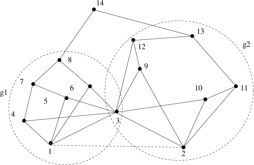
By minor modification of Figure 13, we have the following stronger observation.

Observation 4.12

For any graph $G_{s}$ , there exists a 1-path Simple 1-dof Henneberg-I graph $G$ with base non-edge $f$ such that $G$ has low sampling complexity on $f$ and $G_{s}$ is a minor of $G$ .

Proof We only need to prove the case that $G_{s}$ is an arbitrary clique $K_{m}$ . To do that, we change the subgraph $G_{1}$ in Figure 13 such that $K_{m}$ is a minor of $G_{1}$ . If we can do this, the proof follows since by using the same argument as proof for Observation 4.11, we additionally have: both $G_{1}$ and $G_{2}$ are Henneberg-I graphs with base edge $(v_{1},v_{3})$ and $(v_{2},v_{3})$ respectively; there are only two extreme graphs which are both wellconstrained and Triangle-decomposable so $G$ has low sampling complexity on $(v_{1},v_{2})$ .

We prove by induction that we can construct a 1-path Henneberg-I graph $G_{1}$ with base edge $(v_{1},v_{3})$ such that $G_{1}$ can be reduced to $K_{m}$ by edge contractions. The base cases ( $m=1,2,3$ ) have been shown in Figure 13. As the induction hypothesis, we assume that we can construct a 1-path Henneberg-I graph $G_{1}^{m}$ with base edge $(v_{1},v_{3})$ such that $G_{1}^{m}$ can be reduced to $K_{m}$ by edge contractions. Now we prove the induction step for $K_{m+1}$ . We start from $G_{1}^{m}$ to construct $G_{1}^{m+1}$ . We pick $m$ vertices $u_{1},\cdots,u_{m}$ from $G_{1}^{m}$ containing the last constructed vertex of $G_{1}^{m}$ and additionally such that they map to distinct vertices in the contracted graph $K_{m}$ . We add a vertex $w_{1}$ by a Henneberg-I step with $u_{1}$ and $u_{2}$ as base vertices. Then we add a vertex $w_{2}$ by a Henneberg-I step with $w_{1}$ and $u_{2}$ as base vertices and so on. Finally we add $w_{m-1}$ by Henneberg-I step with $w_{m-2}$ and $u_{m}$ as base vertices to get $G_{1}^{m+1}$ (Please refer to Figure 14 for a $K_{5}$ example). Clearly, $G_{1}^{m+1}$ is a Henneberg-I graph with base edge $(v_{1},v_{3})$ . Then by contracting all the edges that have at least one vertex other than $u_{1}$ , $\cdots$ , $u_{m}$ and $w_{m-1}$ , we get a $K_{m+1}$ . Thus, we have proved that $G_{1}^{m+1}$ is a Henneberg-I graph and can be contracted to $K_{m+1}$ . $\Box$

Observation 4.13

There exists a triangle-free Simple 1-dof Henneberg-I graph with base non-edge $f=(v_{1},v_{2})$ such that $G$ has low sampling complexity on $f$ and $G$ has both $K_{3,3}$ and/or $C_{3}\times C_{2}$ minor.

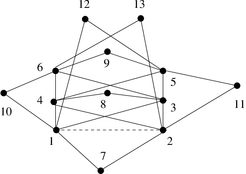
Proof We give such a graph $G$ in Figure 15. The Simple 1-dof Henneberg-I graph is constructed with base non-edge $(v_{1},v_{2})$ and it is not a 1-path. We can verify that all the extreme graphs are in fact Henneberg-I graphs so they are Triangle-decomposable. This shows that $G$ has low sampling complexity on $f$ . If we contract all the edges that have at least one vertex other than $v_{1}$ , $v_{2}$ , $v_{3}$ , $v_{4}$ , $v_{5}$ and $v_{6}$ , we can get a clique $K_{6}$ , so $G$ has both $K_{3,3}$ and $C_{3}\times C_{2}$ minors. $G$ has all the required properties of the observation. $\Box$

4.2.4 Graph characterization for 1-path Simple 1-dof Henneberg-I graph

Despite the obstacles to obtaining a forbidden minor characterization when the “triangle-free” restriction is removed, the following theorem gives a characterization of 1-path 1-dof Simple Henneberg-I graphs $G$ that have low sampling complexity.

Theorem 4.14

Given a 1-path Simple 1-dof Henneberg-I graph $G$ with specified base non-edge $(v_{1},v_{2})$ , if $G$ has low sampling complexity on $v_{1},v_{2}$ then the number of vertices directly constructed using $v_{1}$ and $v_{2}$ as base vertices is 1 or 2. If it is 2, $G$ has low sampling complexity on $(v_{1},v_{2})$ if and only if the following hold: (1) either $v_{1}$ or $v_{2}$ has a degree of 2; (2) if $v_{3}$ and $v_{4}$ are the only vertices directly constructed on $v_{1}$ and $v_{2}$ and the degrees of both $v_{1}$ and $v_{2}$ are 2, 1-path Simple 1-dof Henneberg-I graph $G\setminus\{v_{1},v_{2}\}$ must have low sampling complexity on base non-edge $(v_{3},v_{4})$ ; (3) if $v_{3}$ and $v_{4}$ are the only vertices directly constructed on $v_{1}$ and $v_{2}$ and only one of $v_{1}$ and $v_{2}$ has degree of 2, without loss of generality say $v_{2}$ , then $G\setminus\{v_{2}\}$ has to be a Simple 1-dof 1-Path Henneberg-I graph that has low sampling complexity on base non-edge $(v_{3},v_{4})$ .

Proof For (1), assume there are $m$ vertices in $G$ that are directly constructed with $v_{1}$ and $v_{2}$ as base vertices. By Lemma 4.8 (1.a), $m<3$ . When $m=2$ , assume $v_{3}$ and $v_{4}$ are constructed with $v_{1}$ and $v_{2}$ as base vertices. Since $v_{1}$ and $v_{2}$ are adjacent to both $v_{3}$ and $v_{4}$ , so both $deg(v_{1})$ and $deg(v_{2})$ are at least 2. By Lemma 4.8 1.b, $deg(v_{1})$ and $deg(v_{2})$ cannot be both greater than 2, so either $v_{1}$ or $v_{2}$ has degree of two.

By Lemma 4.9 (1.a) and (1.b) we have (2) and by Lemma 4.9 (2.a) and (2.b) we have (3). $\Box$

Remark: Theorem 4.14 leaves the case where the number of vertices directly constructed using $v_{1}$ and $v_{2}$ as base vertices is exactly 1. Such graphs of low sampling complexity are captured in Figure 16. The graph characterization for this type of graphs is complicated and appears in [8].

The above theorem characterizes the Simple, 1-dof, 1-path Henneberg-I graphs that have Triangle-decomposable extreme graphs and low sampling complexity. It is natural to ask if the configuration space description for these graphs can also be obtained directly as in Observation 4.10, without actually realizing the extreme graphs. The next observation gives a negative answer.

Observation 4.15

Figure 16 shows an example of a Simple, 1-dof, 1-path Henneberg-I graph with low sampling complexity, for which the interval endpoints in its configuration space cannot directly be obtained by the method of quadrilateral diagonal interval mapping (in Observation 4.10).

Proof In Figure 16, the graph is a 1-path 1-dof Henneberg-I graph that has low sampling complexity on base non-edge $(v_{1},v_{2})$ . However, we cannot find a sequence of quadrilaterals such that we can use a quadrilateral diagonal interval mapping. For example, if we start from $\triangle(v_{25},v_{26},v_{27})$ and get an interval for $\delta^{*}(v_{25},v_{26})$ , then we have no further quadrilaterals to proceed. $\Box$

4.3 Characterizing parameter choices: all base edges yield equally efficient configuration spaces

We show an interesting quantifier exchange theorem for Henneberg-I graphs. Besides providing a characterization of all possible parameters that yield efficient configuration spaces, the theorem illustrates the robustness of our definition of low sampling complexity.

Theorem 4.16

For a Henneberg-I graph $H$ , consider each possible base edge $f$ that gives a Henneberg construction for $H$ . Let $H_{f}$ be the Simple 1-dof Henneberg-I graph with base non-edge $f$ . Then either $\Phi_{f}^{2}(H_{f},\delta)$ has low sampling complexity for all base edges $f$ of $H$ or for none of them. See Figure 15.

Proof We prove by contradiction. Suppose the proposition is not true, then we can find ¨¢ set of Simple 1-dof Henneberg-I graphs such that for each of them we can find two base non-edges such that it has low sampling complexity on one base non-edge while does not have sampling complexity on the other. We pick a graph $G$ among this set such that the number of the vertices of $G$ is the minimum. If there is any tie, we break the tie arbitrarily. Without loss of generality, we assume that $G$ has two base non-edges $f_{1}=(v_{1},v_{2})$ and $f_{2}=(v_{3},v_{4})$ and $G$ has low sampling complexity on $f_{1}$ but does not have low sampling complexity on $f_{2}$ . Clearly $f_{1}$ and $f_{2}$ cannot be the same and $G$ has at least 3 vertices.

The proof rests on several claims on the above $G$ , $f_{1}$ and $f_{2}$ which exclude the possibility of minimality.

Claim 4.17

For any vertex of $G$ other than $v_{1}$ , $v_{2}$ , $v_{3}$ and $v_{4}$ cannot have degree 2.

Proof To the contrary, suppose a vertex $v_{n}$ has degree 2. We used $G^{\prime}$ to denote the graph we get by removing $v_{n}$ from $G$ . Without loss of generality, suppose $v_{n}$ is constructed with $u_{n}$ and $w_{n}$ as base vertices. If $G$ has a wellconstrained subgraph which includes both $u_{n}$ and $w_{n}$ , by Fact 4.1 the subgraph is a Henneberg-I graph and also a 2-sum component of $G$ . So $G^{\prime}$ will be also a Henneberg-I graph with two base non-edges $f_{1}$ and $f_{2}$ and just like $G$ , $G^{\prime}$ has low sampling complexity on $f_{1}$ but does not have low sampling complexity on $f_{2}$ . Now we consider the case that $G$ does not have a wellconstrained subgraph which include both $u_{n}$ and $w_{n}$ . In this case, since $G$ has low sampling complexity on $f_{1}$ , it follows that $G\cup(u_{n},w_{n})$ is Triangle-decomposable. Compare the extreme graphs associated with $G$ and $(v_{3},v_{4})$ and the extreme graphs associated with $G^{\prime}$ and $(v_{3},v_{4})$ , the former has one more extreme graph $G\cup(v_{1},v_{2})$ . $G$ does not have low sampling complexity on $f_{2}=(v_{3},v_{4})$ , so one extreme graph associated with $(G,f_{2})$ is not Triangle-Decomposable. Now $G\cup(v_{i},v_{j})$ is Triangle-Decomposable, so one extreme graph associated with $(G^{\prime},f_{2})$ must not be Triangle-Decomposable, thus, $G^{\prime}$ must have one extreme graph which is not Triangle-Decomposable such that $G^{\prime}$ does not have low sampling complexity on $f_{2}$ . In both cases, $G^{\prime}$ is a Henneberg-I graph with base non-edges $f_{1}$ and $f_{2}$ and just like $G$ , $G^{\prime}$ has low sampling complexity on $f_{1}$ but does not have low sampling complexity on $f_{2}$ . This violates the minimality of $G$ , so our assumption is incorrect and no vertex of $G$ other than $v_{1}$ , $v_{2}$ , $v_{3}$ and $v_{4}$ can have degree 2. $\Box$

Claim 4.18

At least one of $deg(v_{1})$ and $deg(v_{2})$ is 2; similarly, at least one of $deg(v_{3})$ and $deg(v_{4})$ is 2.

Proof Since $G\cup f_{1}$ is a Henneberg-I graph with base non-edge $(v_{1},v_{2})$ (and $G$ has at least 3 vertices), so there is at least one vertex other than $v_{1}$ and $v_{2}$ which has degree of 2. From (1), any vertex other than $v_{1}$ , $v_{2}$ , $v_{3}$ and $v_{4}$ cannot have degree 2, so either $deg(v_{3})$ or $deg(v_{4})$ is 2 since $v_{3}$ and $v_{4}$ are the only vertices other than $v_{1}$ and $v_{2}$ which can have degree 2. Similarly, at least one of $deg(v_{3})$ or $deg_{v_{4}}$ is 2. Without loss of generality we suppose that $deg(v_{1})$ and $deg(v_{3})$ are 2. $\Box$

Claim 4.19

There is only one vertex constructed with $v_{1}$ and $v_{2}$ as base vertices.

Proof In Claim 4.18, we proved that at least one of $deg(v_{1})$ and $deg(v_{2})$ is two we assume that $deg(v_{1})$ is 2 so the number of vertices constructed with $v_{1}$ and $v_{2}$ as base vertices is at most two. We can show by contradiction that this number is not exactly 2. Suppose $v_{5}$ and $v_{6}$ are the two vertices constructed with $v_{1}$ and $v_{2}$ as base vertices. By Lemma 4.9(2.a), $(v_{5},v_{6})$ is also a base non-edge for $G$ . $G$ has low sampling complexity on $(v_{1},v_{2})$ , so by Lemma 4.9(1.b or 2.b), $G$ also has low sampling complexity on $(v_{5},v_{6})$ . If $v_{1}$ is different from both $v_{3}$ and $v_{4}$ , we have: $G$ does not have low sampling complexity on $(v_{3},v_{4})$ , $G$ has low sampling complexity on $(v_{5},v_{6})$ , $v_{1}$ has degree 2, and $v_{1}$ is different from $v_{3}$ , $v_{4}$ , $v_{5}$ and $v_{6}$ . This contradicts to Cliam 4.17, so we only need to consider the case that $v_{1}$ is the same as $v_{3}$ or $v_{4}$ . Without loss of generality, we assume that $v_{1}$ is the same as $v_{3}$ . $G$ is a 1-dof Henneberg-I graph with base non-edge $(v_{3},v_{4})$ and $G$ has at least 3 vertices, so at least one vertex of $G$ other than $v_{3}$ and $v_{4}$ has degree 2. By Cliam 4.17, only $v_{1}$ , $v_{2}$ , $v_{3}$ and $v_{4}$ can have degree 2, so $deg(v_{2})$ has to be 2. Now, $G$ has low sampling complexity on $(v_{5},v_{6})$ , $G$ does not have low sampling complexity on $(v_{3},v_{4})$ , vertex $v_{2}$ has degree of 2 and $v_{2}$ is different from $v_{3}$ , $v_{4}$ , $v_{5}$ and $v_{6}$ . This again contradicts to Cliam 4.17 thus proves the claim. $\Box$

[Theorem 4.16 Continued] By Claim 4.19 there is only one vertex constructed with $v_{1}$ and $v_{2}$ as base vertices, without loss of generality, suppose $v_{9}$ is such a vertex. Consider the Henneberg-I step that immediately follows $v_{9}\triangleleft(v_{1},v_{2})$ . Since $v_{9}$ is the vertex constructed with $v_{1}$ and $v_{2}$ as base vertices, the base vertices for the next Henneberg-I step are either $v_{1}$ and $v_{9}$ or $v_{2}$ and $v_{9}$ . Since we have labeled $v_{1}$ as the vertex which has degree of 2, we have to differentiate these two cases. In Claim 4.20 we discuss the case in which the next Henneberg-I step is $v_{10}\triangleleft(v_{1},v_{9})$ and in Claim 4.21 we discuss the case in which the next Henneberg-I step is $v_{10}\triangleleft(v_{2},v_{9})$ .

Claim 4.20

If $v_{9}$ is the only vertex constructed with $v_{1}$ and $v_{2}$ as base vertices and $deg(v_{1})$ is 2, then no vertex can be constructed with $v_{1}$ and $v_{9}$ as base vertices.

Proof Refer to Figure 17, $(v_{2},v_{10})$ is also a base non-edge for Simple 1-dof Henneberg-I graph $G$ . Further $G$ has low sampling complexity on $(v_{2},v_{10})$ since $G$ has low sampling complexity on $(v_{1},v_{2})$ . This is a result which is similar to Lemma 4.9 (1.b) and can be proved by comparing all the possible extreme graphs. For any extreme graph corresponding to $(v_{2},v_{10})$ , there is an extreme graph corresponding to $(v_{1},v_{2})$ which has one extra Henneberg-I step $v_{1}\triangleleft(v_{9},v_{10})$ . $G$ has low sampling complexity on $(v_{1},v_{2})$ , so all the extreme graphs corresponding to $(v_{1},v_{2})$ are triangle decomposable. Thus, all the extreme graphs corresponding to $(v_{2},v_{10})$ are also triangle decomposable since removing vertices from a triangle decomposable graph by inverse Henneberg-I steps keeps the graph still triangle decomposable. So, $G$ has low sampling complexity on $(v_{2},v_{10})$ .

Note that $G$ has does not have low sampling complexity on $(v_{3},v_{4})$ and $deg(v_{1})$ is 2. By Claim 4.17, $v_{1}$ cannot be different from both $v_{3}$ and $v_{4}$ (Figure 17(a)). So we only need to consider the case $v_{1}$ is coincident with $v_{3}$ or $v_{4}$ . Although we labeled $v_{3}$ as the vertex with degree of 2 but we do not use this property here, so we suppose $v_{1}$ is coincident with $v_{4}$ .

Since $(v_{3},v_{4})$ is a base non-edge for $G$ and $v_{4}$ (just like $v_{1}$ ) is only adjacent to $v_{9}$ and $v_{10}$ , so $v_{3}$ must be adjacent to either $v_{9}$ (Figure 17(b)) or $v_{10}$ (Figure 17(c)) in order to guarantee the Henneberg-I step with $v_{3}$ and $v_{4}$ as base vertices is possible. For Figure 17(b), $(v_{3},v_{10})$ is a base non-edge for $G$ since $(v_{3},v_{4})$ is a base non-edge for $G$ . If we compare the extreme graphs corresponding to $(v_{3},v_{10})$ with the extreme graphs corresponding to $(v_{3},v_{4})$ , the only difference is: the extreme graph in the latter case has one more Henneberg-I step $v_{4}\triangleleft(v_{9},v_{10})$ . Note that removing/adding a Henneberg-I step to a graph does not change triangle decomposability. Now $G$ does not have low sampling complexity on $(v_{3},v_{4})$ , so $G$ does not have low sampling complexity on $(v_{3},v_{10})$ . Now we have: $G$ does not have low sampling complexity on $(v_{3},v_{10})$ , $G$ has low sampling complexity on $(v_{1},v_{2})$ , $v_{1}$ has degree of 2 and $v_{1}$ is different from $v_{2}$ , $v_{3}$ , $v_{9}$ and $v_{10}$ . This contradicts to the result in Claim 4.17, so the case shown in Figure 17(b) is impossible. We can use the same argument for the case shown in Figure 17(c) and get: $G$ does not have low sampling complexity on $(v_{3},v_{9})$ , $G$ has low sampling complexity on $(v_{1},v_{2})$ , $v_{1}$ has degree of 2 and $v_{1}$ is different from $v_{2}$ , $v_{3}$ , $v_{9}$ and $v_{10}$ . This again contradicts to Claim 4.17, so the case shown in Figure 17(c) is also impossible. Now we have shown that we cannot have a Henneberg-I step $v_{10}\triangleleft(v_{1},v_{9})$ . $\Box$

Claim 4.21

If $v_{9}$ is the only vertex constructed with $v_{1}$ and $v_{2}$ as base vertices and $deg(v_{1})$ is 2, then no vertex can be constructed with $v_{2}$ and $v_{9}$ as base vertices either.

Proof Otherwise, let $v_{10}$ be constructed with $v_{2}$ and $v_{9}$ as base vertices(see Figure 18 and Figure 19).

Let $v_{12}$ denote the other vertex that $v_{1}$ is adjacent (we know that $v_{1}$ is adjacent to $v_{9}$ ). Observe that $(v_{1},v_{2})$ is a base non-edge for $G$ , so $v_{1}$ must be one of the two base vertices for $v_{12}$ ’s construction. Denote the other vertex by $v_{11}$ . Clearly, before $v_{12}$ is constructed, we must have constructed a 1-path Henneberg-I graph with $(v_{2},v_{9})$ as base edge and $v_{11}$ as the last vertex. We denote this 1-path Henneberg-I graph by $G_{1}$ and mark it by a dashed circle in Figure 18.

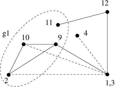
We can show that $v_{1}$ has to be different from $v_{3}$ and $v_{4}$ . Since $G$ is simple 1-dof Henneberg-I graph with base non-edge $(v_{3},v_{4})$ , at least one vertex other than $v_{3}$ and $v_{4}$ should have degree 2. By Claim 4.17, $v_{1}$ and $v_{2}$ are the only possible vertices with degree of 2. If $v_{1}$ is $v_{3}$ or $v_{4}$ , $deg(v_{2})$ is 2. But $deg(v_{2})$ cannot be 2 by Claim 4.20, so we have proved that $v_{1}$ has to be different from $v_{3}$ and $v_{4}$ and $deg(v_{2})$ is not 2(see Figure 18).

For the remaining cases, we will use Claim 4.17 to target the impossbility which is stated in the laim we want to prove. To do that, we change the edges of $G$ to get a new graph $G$ such that: $G^{\prime}$ has low sampling complexity on base non-edge $f_{3}$ ; $G^{\prime}$ does not have low sampling complexity on base non-edge $(v_{3},v_{4})$ ; $v_{1}$ is different from $v_{3}$ , $v_{4}$ and the two vertices of $f_{3}$ .

If we consider the Henneberg-I sequence starting from $(v_{1},v_{2})$ , $G_{1}$ is a Henneberg-I graph with $(v_{2},v_{9})$ as base vertice and the last vertex is $v_{11}$ . This means that any vertex in $G_{1}$ other than $v_{2}$ , $v_{9}$ and $v_{11}$ do not have degree 2. Consider how we can construct $G_{1}$ in the Henneberg-I sequence starting from $(v_{3},v_{4})$ . Recall each Henneberg-I step involves 1 vertex and 2 edges. By using the same dof counting method that used for Fact 4.1, there must be an edge between the first two vertices in $G_{1}$ , without loss of generality we assume that the first vertex is $v_{13}$ and the second is $v_{14}$ . So, $G_{1}$ has to be a Henneberg-I graph(may not be 1-path) with base edge $(v_{13},v_{14})$ .

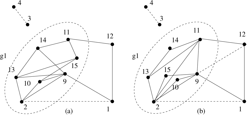
Now we modify $G_{1}$ to get $G_{1}^{\prime}$ such that we get the $G^{\prime}$ that we expect. We keep all the vertices in $G_{1}$ but remove all the edges. Our objective is to add edges to get a new graph $G_{1}^{\prime}$ such that $G_{1}^{\prime}$ is a Henneberg-I graph with both $(v_{2},v_{9})$ and $(v_{13},v_{14})$ as base edges and $G_{1}^{\prime}$ contains edges $(v_{2},v_{11})$ and $(v_{9},v_{11})$ . To achieve this, we first add edges $(v_{2},v_{9})$ , $(v_{2},v_{11})$ and $(v_{9},v_{11})$ . Then we consider adding edges for $v_{13}$ and $v_{14}$ : if both $v_{13}$ and $v_{14}$ are among $v_{2}$ , $v_{9}$ or $v_{11}$ , we do not add any edge; if exactly one of $v_{13}$ and $v_{14}$ is one of $v_{2}$ , $v_{9}$ or $v_{11}$ , we add edges $(v_{13},v_{14})$ and another edge between $v_{11}$ and whichever of $v_{13}$ and $v_{14}$ is not one of $v_{2}$ , $v_{9}$ or $v_{11}$ ; if neither of $v_{13}$ and $v_{14}$ is one of $v_{2}$ , $v_{9}$ or $v_{11}$ , we add edges $(v_{13},v_{2})$ , $(v_{13},v_{11})$ $(v_{14},v_{13})$ and $(v_{14},v_{11})$ . Finally for each vertex $u$ in $G_{1}$ other than $v_{2}$ , $v_{9}$ , $v_{11}$ , $v_{13}$ and $v_{14}$ , we add one edge between $u$ and $v_{2}$ and another one between $u$ and $v_{9}$ . We use $G_{1}^{\prime}$ to denote this new subgraph that replaces $G_{1}$ and $G^{\prime}$ for the entire graph. By the manner in which we add edges, our objective is achieved: $G_{1}^{\prime}$ is Henneberg-I graph with both $(v_{2},v_{9})$ and $(v_{13},v_{14})$ as base edges and also contains edges $(v_{2},v_{11})$ and $(v_{9},v_{11})$ .

Now observe that both $(v_{1},v_{2})$ and $(v_{3},v_{4})$ are still base non-edges for $G^{\prime}$ . Further, $(v_{9},v_{12})$ is also a base non-edge for $G$ . Now we consider whether $G^{\prime}$ has low sampling complexity on $(v_{9},v_{12})$ and $(v_{3},v_{4})$ . To do that, we refer to Theorem 1 proved in [7]: if a graph is Triangle-decomposable, we can perform the cluster merging (inverse operation of triangle-decomposition) in any order(a Church-Rosser Property) but finally we get one cluster which is the same as the whole graph. So for any given graph, if we replace one of its Triangle-decomposable subgraphs by another triangle decomposable subgraph while keeping the vertices unchanged, the graph preserves Triangle-decomposability. Here in our transform, both $G_{1}$ and $G_{1}^{\prime}$ are Henneberg-I graphs and thus both are Triangle-decomposable. Compare the extreme graphs corresponding to $G$ and $G^{\prime}$ for which base non-edge is chosen as $(v_{1},v_{2})$ .

Observe that we are only interested in well-constrained extreme graphs. By Fact 4.3, an extreme graph corresponding to the Henneberg-I step $v\triangleleft(u,w)$ is wellconstrained if and only if $u$ and $w$ are not in any wellconstrained subgraph. Observe that the difference between $G$ and $G^{\prime}$ is exactly the difference between $G_{1}$ and $G_{1}^{\prime}$ . Both $G_{1}$ and $G_{1}^{\prime}$ are wellconstrained, so in the comparison of extreme graphs we do not need to consider extreme graphs corresponding to the Henneberg-I steps inside $G_{1}$ and $G_{1}^{\prime}$ .

For all the other Henneberg-I steps outside $G_{1}$ and $G_{1}^{\prime}$ , the difference between the extreme graphs for $G$ and $G^{\prime}$ is exactly the difference between $G_{1}$ and $G^{\prime}$ . This proves $G^{\prime}$ has low sampling complexity on $(v_{1},v_{2})$ since $G$ has low sampling complexity on $(v_{1},v_{2})$ . Similarly, we can show that $G^{\prime}$ does not have low sampling complexity on $(v_{3},v_{4})$ since $G$ does not have low sampling complexity on $(v_{3},v_{4})$ . Now verifying Figure 19 again, $(v_{9},v_{12})$ is also a base non-edge for $G^{\prime}$ . By comparison of extreme graphs as we did in Claim 4.20, $G^{\prime}$ has low sampling complexity on $(v_{1},v_{2})$ since $G^{\prime}$ has low sampling complexity on $(v_{9},v_{12})$ . This contradicts to Claim 4.17, so we have proved when $v_{9}$ is the only vertex constructed with $v_{1}$ and $v_{2}$ as base vertices and $deg(v_{1})$ is 2, then no vertex can be constructed with $v_{2}$ and $v_{9}$ as base vertices either. $\Box$

[Theorem 4.16 Continued] Now we can put all the 5 claims together. We assume that $G$ has low sampling complexity on base non-edge $(v_{1},v_{2})$ but does not have low sampling complexity on base non-edge $(v_{3},v_{4})$ . We also assume that the number of vertices in $G$ is minimum among all the graphs with this property. In Claim 4.17 to Claim 4.21, we discuss what properties such a $G$ should have in order to keep the minimality of the number of vertices. In Claim 4.17 we show that any vertex other than $v_{1}$ , $v_{2}$ , $v_{3}$ and $v_{4}$ cannot have degree 2; in Claim 4.18, we show at least one of $deg(v_{1})$ and $deg(v_{2})$ (resp. at least one of $deg(v_{3})$ and $deg_{v_{4}}$ ) is 2 and without loss of generality we assume that $deg(v_{1})$ and $deg(v_{3})$ are 2; in Claim 4.19, we show that there is only vertex that is constructed with $v_{1}$ and $v_{2}$ as base vertices and we denote the vertex by $v_{9}$ ; the result in Claim 4.19 narrows the Henneberg-I step that follows $v_{9}\triangleleft(v_{1},v2)$ to either $v_{10}\triangleleft(v_{2},v_{9})$ or $v_{10}\triangleleft(v_{1},v_{9})$ , so in Claim 4.20 we show that $v_{10}\triangleleft(v_{1},v_{9})$ is infeasible; finally Claim 4.21 shows that the only remaining possibility namely $v_{10}\triangleleft(v_{2},v_{9})$ results in a consequence that contradicts to Claim 4.17. This implies no minimal graph $G$ can exist that contradicts the conditions of the theorem, thus proving Theorem 4.16. $\Box$

5 Conclusions and Future Work

By studying the configuration spaces of Simple 1-dof Henneberg-I graphs, we have taken the next step in a systematic and graded program laid out in [8] - for the combinatorial characterizations of efficient configuration spaces of underconstrained 2D Euclidean Distance Constraint Systems (resp. frameworks). In particular, the results presented here go the next step beyond graphs with connected and convex configuration spaces studied in [17].

A generalization of the results presented here from Henneberg-1 graphs to the larger class of Tree- or Triangle-decomposable graphs appears in [8] and [18].

As immediate future work, it would be desirable to give a cleaner combinatorial characterization of low sampling complexity for configuration spaces of 1-path Simple 1-dof Henneberg-I graphs. I.e, it would be desirable to improve the characterization of Theorem 4.14. The next natural continuation is to study configuration spaces of graphs with $k$ dofs ( $k>1$ ) obtained by deleting $k$ edges from Henneberg-I or Tree- or Triangle-decomposable graphs.

References

[1] A. Y. Alfakih, A. Khandani and H. Wolkowicz. Solving Euclidean Distance Matrix Completion Problems via Semidefinite Programming. Comput. Optim. Appl., 12:13–30, 1999.
[2] M. Bădoiu, K. Dhamdhere, A. Gupta, Y. Rabinovich, H. Räcke, R. Ravi and A. Sidiropoulos. Approximation algorithms for low-distortion embeddings into low-dimensional spaces. SODA ’05: Proceedings of the sixteenth annual ACM-SIAM Symposium on Discrete Algorithms, page 119–128, 2005.
[3] Pratik Biswas, Tzu-Chen Lian, Ta-Chung Wang and Yinyu Ye. Semidefinite programming based algorithms for sensor network localization. ACM Trans. Sen. Netw., 2(2):188–220, 2006.
[4] A. Cayley. A theorem in the geometry of position. Cambridge mathematical Journal., II:267–271, 1841.
[5] G.M. Crippen and T.F. Havel. Distance Geometry and Molecular Conformation. Chemometrics Series, 15, Taunton, Somerset, England: Research Studies Press, 1998.
[6] I. Fudos and C. M. Hoffmann. A graph-constructive approach to solving systems of geometric constraints. ACM Trans. on Graphics, pp. 179–216, 1997.
[7] I. Fudos and C. M. Hoffmann. Correctness proof of a geometric constraint solver. Int. J. Comput. Geom. Appl., 6:405–420, 1996.
[8] H. Gao. Geometric Under-Constraints. Ph.D. thesis, University of Florida, Aug. 2008.
[9] H. Gao, and M. Sitharam. Combinatorial Classification of 2D Underconstrained Sytems. Proceedings of the Seventh Asian Symposium on Computer Mathematics (ASCM 2005), Sung-il. Pae. and Hyungju. Park., Eds., 2005, pp. 118–127.
[10] J. E. Graver, B. Servatius, and H. Servatius. Combinatorial Rigidity. Graduate Studies in Math., AMS, 1993.
[11] Robert Joan-Arinyo, Antoni Soto-Riera, S. Vila-Marta and Josep Vilaplana-Pasto. Transforming an under-constrained geometric constraint problem into a well-constrained one. Symposium on Solid Modeling and Applications 2003, pages 33–44, 2003.
[12] G. Laman. On graphs and rigidity of plane skeletal structures. J. Engrg. Math., vol. 4, page 331–340, 1970.
[13] R. Loos Computing in algebraic extensions. In Buchberger Collins, Loos, Albrecht Eds. Computer Algebra: symbolic and algebraic computation, Springer Verlag page 173–187, 1983.
[14] Hilderick A. van der Meiden and Willem F. Bronsvoort. A constructive approach to calculate parameter ranges for systems of geometric constraints. Computer-Aided Design, 38(4):275–283,200
[15] John C. Owen and Steve C. Power. The nonsolvability by radicals of generic 3-connected planar graphs. Transactions of AMS, 359(5):2269–2303, 2006.
[16] M. Sitharam. Graph based geometric constraint solving: problems, progress and directions. in AMS-DIMACS volume on Computer Aided Design, D. Dutta, R. Janardhan, and M. Smid, Eds., 2005.
[17] M. Sitharam and H. Gao. Characterizing graphs with convex and connected configuration spaces. arXiv:0809.3935 [cs.CG].
[18] M. Sitharam and H. Gao “Characterizing 1-Dof Tree-Decomposable graphs with efficient configuration space,” in preparation.
[19] G.F. Zhang and X.S. Gao. Well-constrained Completion and Decomposition for Under-constrained Geometric Constraint Problems. International Journal of Computational Geometry and Applications, pages 461–478, 2006.