Precision $B_{c}$ and $B_{s}$ mass calculations

The precise calculation of the charm and bottom spectra is an important goal of lattice QCD for several reasons:

• •

  There are many ‘gold-plated’ states: narrow, stable, and experimentally accessible.

• •

  The splittings in heavionium have particularly good properties for determining the lattice scale.

• •

  It is an important test of the actions used for $b$ and $c$, which can then be used to calculate decay constants which in turn are crucial for determining CKM matrix elements.

• •

  Control of systematic errors are well developed in calculations of the $B$ and $D$ spectrum on the lattice due to relative insensitivity to heavy-quark polarisation effects and to light quark masses.

The Highly Improved Staggered Quark (HISQ) action [1, 2] allows unprecedented control of discretization errors in numerical lattice calculations. We use HISQ $s$ and $c$ valence quarks with NRQCD $b$ quarks on MILC lattices with $N_{f}=2+1$ flavors of ASQTAD sea quarks to calculate the masses of the $B_{s}$ and $B_{c}$ mesons.

For increased statistics, we use random sources $\eta(x,t_{0})$, defined as a three-component random complex unit-vector defined on each point in the source time slice $t_{0}$. These are the sources for the inversion of the HISQ strange and charmed valence quark propagators. The HISQ propagators, being staggered, are spinless and we need to convert them to 4-component propagators to combine with NRQCD propagators in a $b$-light correlator. This is readily done at the sink by multiplying by the standard staggered-to-naive transformation $\Omega(x)=\prod_{i}\gamma_{i}^{x_{i}}$. Since the propagator source disappears once the propagator is made, the $\Omega$ factors needed at the source (when a random wall is used) must be transferred to the source of the heavy quark propagator and how to do this is described below.

NRQCD propagators are then made from a source which includes the same random wall with which the HISQ propagators are made, plus the $\Omega$ factors and in addition different Gaussian smearing factors of varying radii $r_{i}$ chosen to allow improved overlap with the ground state $B_{s}$ and $B_{c}$ mesons so that their energies can be extracted accurately at early correlator times. We therefore initialise $N_{\rm smear}$ NRQCD $b$ propagators by setting

and evolve with

We use an improved lattice NRQCD Hamiltonian [3]:

Finally, at each time-slice, we combine the $N_{\rm smear}$ NRQCD propagators and the valence $s$ or $c$ quark propagator with the same smearing functions at the sink end, giving us $N_{\rm smear}\times N_{\rm smear}$ $B_{s}$ and $B_{c}$ meson correlators.

The expression for the variance of the $B_{s}$ correlator

contains in it propagators for $\overline{b}\overline{s}bs$ four-quark states. The lightest combination on the lattice is ${\eta_{b}}+{\eta_{s}}$. Therefore the error on the propagator falls like $e^{-\frac{1}{2}(M_{\eta_{b}}+M_{\eta_{s}})t}$ while the signal falls like $e^{-M_{B_{s}}t}$, as can be seen in Figure 1. So the signal-to-noise ratio degrades exponentially by the mass difference seen in the figure. This degradation is worse than for $D_{s}$ states and necessitates smeared sources to be able to fit propagators to small $t$ values. Figure 1 also illustrates that effective masses of propagators $G_{B_{s}}(i,i;t-t_{0})$ with Gaussian smearing with radius 2 and 4 ($G2G2$ and $G4G4$) approach the $M_{B_{s}}$ plateau rapidly compared to the local source-sink combination ($L0L0$).

We fit the measured $B_{s}$ and $B_{c}$ correlators to the form

where $i$ and $j$ respectively index the source and sink smearing functions. The second term is an oscillating parity partner state. We perform simultaneous Bayesian fits of the $G_{\rm meson}(i,j;t-t_{0})$, looking for stability with respect to fit range and $N_{\exp}$.

Since the NRQCD Hamiltonian does not include a mass term, there is a shift in the energy of the $p=0$ states relative to the continuum mass. To correct for the energy shift in $M_{B_{s}}$ and $M_{B_{c}}$ we use the relationship:

where $E_{B_{s}}$ or $E_{B_{c}}$ is the ground-state $E_{1}$. $M_{b\overline{b}}$ on the right-hand side is the spin-averaged experimental masses of $b\overline{b}$ states: $M_{b\overline{b}}=(3M_{\Upsilon}+M_{\eta_{b}})/4$, where we use the recent BaBar measurement of the $\Upsilon(1S)$-$\eta_{b}(1S)$ hyperfine splitting [4]. $E_{b\overline{b}}$ is the corresponding spin-averaged lattice energy, calculated with NRQCD $b$ quark propagators on the same configurations [5]. For $M_{B_{c}}$ we also explore two other methods for cancelling the energy shift:

where $M_{c\overline{c}}=(3M_{\psi}+M_{\eta_{c}})/4$, and $E_{c\overline{c}}$ is the corresponding spin-averaged lattice energy. The final method to extract $M_{B_{c}}$ is

where $M_{\eta_{s}}$ ($E_{\eta_{s}}$) is the mass (lattice energy) of a fictional $s\overline{s}$ pseudoscalar: $M_{\eta_{s}}=\sqrt{2M_{K}^{2}-M_{\pi}^{2}}$.

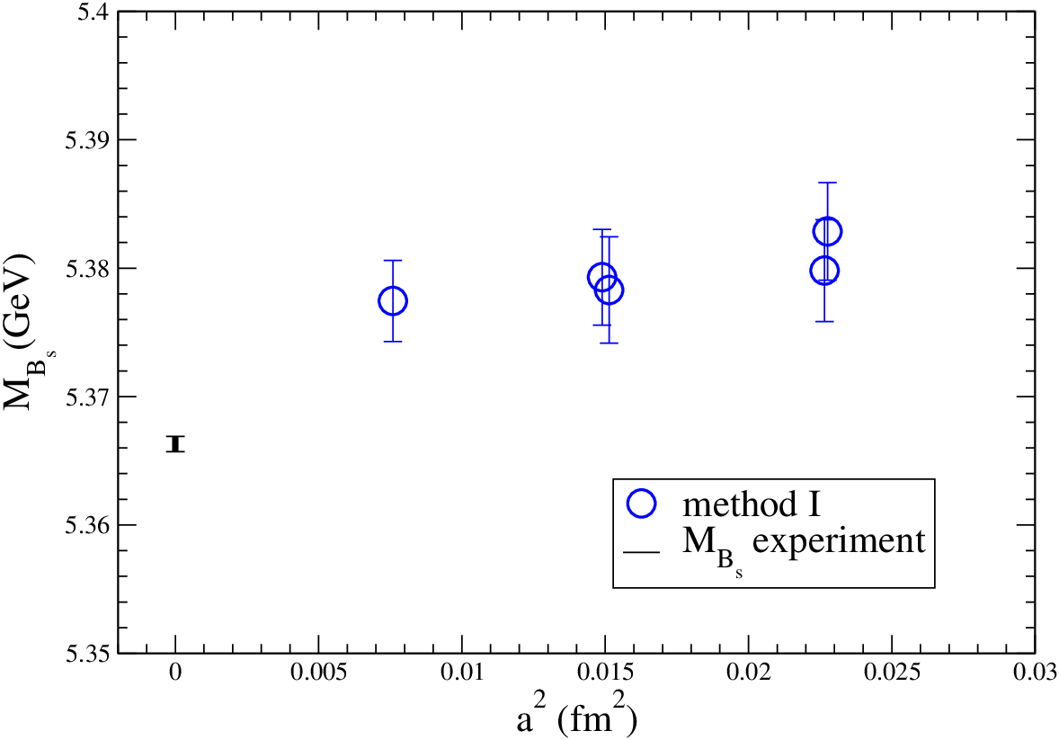
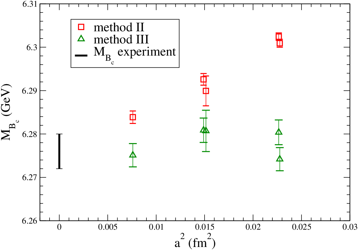
We show results for several ensembles at three lattice spacings and different light sea quark masses for $M_{B_{s}}$ in Figure 2 and $M_{B_{c}}$ in Figure 3. The statistical error (shown in figures) is dominated by the uncertainty in $a^{-1}$. We use MILC $r_{1}/a$ values [7, 8] to set the scale ensemble-by-ensemble. We then convert to physical units with $r_{1}=0.321$fm [3]. An additional systematic error due to the $1.5\%$ uncertainty in $r_{1}$ must be added in at the end with other systematics. Expressions (II) and (III) reduce the uncertainty from errors in $(r_{1}/a)$ by using $(E_{B_{c}}-\frac{1}{2}(E_{b\overline{b}}+E_{c\overline{c}}))_{\rm latt}$ and $(E_{B_{c}}-(E_{B_{s}}+E_{D_{s}}-E_{\eta_{s}}))_{\rm latt}$, which are small relative to the $\left(\right)_{\rm latt}$ quantity in (I).

While preliminary, these results show the potential for precise calculations of $M_{B_{s}}$ and $M_{B_{c}}$ using HISQ valence quarks and NRQCD $b$ quarks on a $2+1$ flavor ASQTAD sea. The lattice results show little sensitivity to sea quark mass. Method (I) and to a lesser extent (II) for $M_{B_{c}}$ show a small dependence on the discretization scale. A slightly mis-tuned $m_{s}$ in the coarse and fine ensembles [8] may contribute some systematic error in $M_{B_{c}}$ values derived from (III), and will be corrected for in future work. Relativistic corrections and electromagnetic effects are two possible sources of systematic error. Future efforts will improve statistics and include finer lattices.

References

- [1] E. Follana et al. [HPQCD Collaboration], Phys. Rev. D 75, 054502 (2007). [arXiv:hep-lat/0610092].
- [2] E. Follana, C. T. H. Davies, G. P. Lepage and J. Shigemitsu [HPQCD Collaboration and UKQCD Collaboration], Phys. Rev. Lett. 100, 062002 (2008) [arXiv:0706.1726 [hep-lat]].
- [3] A. Gray, I. Allison, C. T. H. Davies, E. Dalgic, G. P. Lepage, J. Shigemitsu and M. Wingate, Phys. Rev. D 72, 094507 (2005). [arXiv:hep-lat/0507013].
- [4] B. Aubert et al. [BABAR Collaboration], Phys. Rev. Lett. 101, 071801 (2008) [arXiv:0807.1086 [hep-ex]].
- [5] see I, Kendall, et al., these proceedings.
- [6] I. F. Allison, C. T. H. Davies, A. Gray, A. S. Kronfeld, P. B. Mackenzie and J. N. Simone [HPQCD Collaboration and Fermilab Lattice Collaboration and UKQCD Colla], Phys. Rev. Lett. 94, 172001 (2005). [arXiv:hep-lat/0411027].
- [7] C. W. Bernard et al., Phys. Rev. D 64, 054506 (2001) [arXiv:hep-lat/0104002].
- [8] C. Aubin et al., Phys. Rev. D 70, 094505 (2004) [arXiv:hep-lat/0402030].