A Central Limit Theorem for the SINR at the LMMSE Estimator Output for Large Dimensional Signals

Abla Kammoun ^†^†thanks: $(1)$ Telecom ParisTech (ENST), Paris, France. abla.kammoun@enst.fr Malika Kharouf ^†^†thanks: $(2)$ Telecom ParisTech (ENST) and Casablanca University, Morocco. malika.kharouf@enst.fr Walid Hachem Jamal Najim ^†^†thanks: $(3)$ CNRS / ENST, Paris, France. walid.hachem, jamal.najim@enst.fr

Abstract

This paper is devoted to the performance study of the Linear Minimum Mean Squared Error estimator for multidimensional signals in the large dimension regime. Such an estimator is frequently encountered in wireless communications and in array processing, and the Signal to Interference and Noise Ratio (SINR) at its output is a popular performance index. The SINR can be modeled as a random quadratic form which can be studied with the help of large random matrix theory, if one assumes that the dimension of the received and transmitted signals go to infinity at the same pace. This paper considers the asymptotic behavior of the SINR for a wide class of multidimensional signal models that includes general multi-antenna as well as spread spectrum transmission models.
The expression of the deterministic approximation of the SINR in the large dimension regime is recalled and the SINR fluctuations around this deterministic approximation are studied. These fluctuations are shown to converge in distribution to the Gaussian law in the large dimension regime, and their variance is shown to decrease as the inverse of the signal dimension.

Index Terms:

Antenna Arrays, CDMA, Central Limit Theorem, LMMSE, Martingales, MC-CDMA, MIMO, Random Matrix Theory.

I Introduction

Large Random Matrix Theory (LRMT) is a powerful mathematical tool used to study the performance of multi-user and multi-access communication systems such as Multiple Input Multiple Output (MIMO) digital wireless systems, antenna arrays for source detection and localization, spread spectrum communication systems as Code Division Multiple Access (CDMA) and Multi-Carrier CDMA (MC-CDMA) systems. In most of these communication systems, the $N$ dimensional received random vector ${\bf r}\in{\mathbb{C}}^{N}$ is described by the model

{\bf r}={\boldsymbol{\Sigma}}{\bf s}+{\bf n}

(1)

where ${\bf s}=[s_{0},s_{1},\ldots,s_{K}]^{\mathrm{T}}$ is the unknown random vector of transmitted symbols with size $K+1$ satisfying ${\mathbb{E}}{\bf ss}^{*}={\bf I}_{K+1}$ , the noise ${\bf n}$ is an independent Additive White Gaussian Noise (AWGN) with covariance matrix ${\mathbb{E}}{\bf nn}^{*}=\rho{\bf I}_{N}$ whose variance $\rho>0$ is known, and matrix ${\boldsymbol{\Sigma}}$ represents the known “channel” in the wide sense whose structure depends on the particular system under study. One typical problem addressed by LRMT concerns the estimation performance by the receiver of a given transmitted symbol, say $s_{0}$ .

In this paper we focus on one of the most popular estimators, namely the linear Wiener estimator, also called LMMSE for Linear Minimum Mean Squared Error estimator: the LMMSE estimate $\hat{s}_{0}={\bf g}^{*}{\bf r}$ of signal $s_{0}$ is the one for which the $N\times 1$ vector ${\bf g}$ minimizes ${\mathbb{E}}|\hat{s}_{0}-s_{0}|^{2}$ . If we partition the channel matrix as ${\boldsymbol{\Sigma}}=\left[{\bf y}\ {\bf Y}\right]$ where ${\bf y}$ is the first column of ${\boldsymbol{\Sigma}}$ and where matrix ${\bf Y}$ has dimensions $N\times K$ , then it is well known that vector ${\bf g}$ is given by ${\bf g}=\left({\boldsymbol{\Sigma}}{\boldsymbol{\Sigma}}^{*}+\rho{\bf I}_{N}\right)^{-1}{\bf y}$ . Usually, the performance of this estimator is evaluated in terms of the Signal to Interference plus Noise Ratio (SINR) at its output. Writing the received vector ${\bf r}$ as ${\bf r}=s_{0}{\bf y}+{\bf r}_{\text{in}}$ where $s_{0}{\bf y}$ is the relevant term and ${\bf r}_{\text{in}}$ represents the so-called interference plus noise term, the SINR is given by $\beta_{K}=|{\bf g}^{*}{\bf y}|^{2}/{\mathbb{E}}|{\bf g}^{*}{\bf r}_{\text{in}}|^{2}$ . Plugging the expression of ${\bf g}$ given above into this expression, one can prove that the SINR $\beta_{K}$ is given by the well-known expression:

\beta_{K}={\bf y}^{*}\left({\bf YY}^{*}+\rho{\bf I}_{N}\right)^{-1}{\bf y}\ .

(2)

In general, this expression does not provide a clear insight on the impact of the channel model parameters (such as the load factor $KN^{-1}$ , the power distribution of the transmission data streams, or the correlation structure of the channel paths in the context of multi-antenna transmissions) on the performance of the LMMSE estimator.

An alternative approach, justified by the fluctuating nature of the channel paths in the context of MIMO communications and by the pseudo-random nature of the spreading sequences in spread spectrum applications consists to model matrix ${\boldsymbol{\Sigma}}$ as a random matrix (in this case, $\beta_{K}$ becomes a random SINR). The simplest random matrix model for ${\boldsymbol{\Sigma}}$ , corresponding to the most canonical MIMO or CDMA transmission channels, corresponds to independent and identically distributed (i.i.d.) entries with mean zero and variance $N^{-1}$ . In that case, LRMT shows that when $K\to\infty$ and the load factor $KN^{-1}$ converges to a limiting load factor $\alpha>0$ , the SINR $\beta_{K}$ converges almost surely (a.s.) to an explicit deterministic quantity $\overline{\beta}(\alpha,\rho)$ which simply depends on the limiting load factor $\alpha$ and on the noise variance $\rho$ . As a result, the impact of these two parameters on the LMMSE performance can be easily evaluated [1, 2].

The LMMSE SINR large dimensional behavior for more sophisticated random matrix models has also been thoroughly studied (cf. [1, 3, 4, 5, 6, 7, 8, 9]) and it has been proved that there exists a deterministic sequence $(\overline{\beta}_{K})$ , generally defined as the solution of an implicit equation, such that $\beta_{K}-\overline{\beta}_{K}\to 0$ almost surely as $K\to\infty$ and $\frac{K}{N}$ remains bounded away from zero and from infinity.

Beyond the convergence $\beta_{K}-\overline{\beta}_{K}\to 0$ , a natural question arises concerning the accuracy of $\overline{\beta}_{K}$ for finite values of $K$ . A first answer to this question consists in evaluating the Mean Squared Error (MSE) of the SINR ${\mathbb{E}}|\beta_{K}-\overline{\beta}_{K}|^{2}$ for large $K$ . A further problem is the computation of outage probability, that is the probability for $\beta_{K}-\overline{\beta}_{K}$ to be below a certain level. Both problems can be addressed by establishing a Central Limit Theorem (CLT) for $\beta_{K}-\overline{\beta}_{K}$ . In this paper, we establish such a CLT (Theorem 3 below) for a large class of random matrices ${\boldsymbol{\Sigma}}$ . We prove that there exists a sequence $\Theta_{K}^{2}={\cal O}(1)$ such that $\frac{\sqrt{K}}{\Theta_{K}}(\beta_{K}-\overline{\beta}_{K})$ converges in distribution to the standard normal law ${\cal N}(0,1)$ in the asymptotic regime. One can therefore infer that the MSE asymptotically behaves like $\frac{\Theta_{K}^{2}}{K}$ and that the outage probability can be simply approximated by a Gaussian tail function.

The class of random matrices ${\boldsymbol{\Sigma}}$ we consider in this paper is described by the following statistical model: Assume that

{\boldsymbol{\Sigma}}=\big({\Sigma}_{nk}\big)_{n=1,k=0}^{N,K}=\left(\frac{\sigma_{nk}}{\sqrt{K}}W_{nk}\right)_{n=1,k=0}^{N,K}

(3)

where the complex random variables $W_{nk}$ are i.i.d. with ${\mathbb{E}}W_{nk}=0$ , ${\mathbb{E}}W_{nk}^{2}=0$ and ${\mathbb{E}}|W_{nk}|^{2}=1$ and where $(\sigma_{nk}^{2};\ 1\leq n\leq N;\ 0\leq k\leq K)$ is an array of real numbers. Due to the fact that ${\mathbb{E}}|{\Sigma}_{nk}|^{2}=\frac{\sigma_{nk}^{2}}{K}$ , the array $(\sigma_{nk}^{2})$ is referred to as a variance profile. An important particular case is when $\sigma_{nk}^{2}$ is separable, that is, writes:

\sigma_{nk}^{2}=d_{n}\tilde{d}_{k}\ ,

(4)

where $(d_{1},\ldots,d_{N})$ and $(\tilde{d}_{0},\ldots,\tilde{d}_{K})$ are two vectors of real positive numbers.

Applicative contexts.

Among the applicative contexts where the channel is described appropriately by model (3) or by its particular case (4), let us mention:

•

Multiple antenna transmissions with $K+1$ distant sources sending their signals toward an array of $N$ antennas. The corresponding transmission model is ${\bf r}={\boldsymbol{\Xi}}{\bf s}+{\bf n}$ where ${\boldsymbol{\Xi}}=\frac{1}{\sqrt{K}}{\bf H}{\bf P}^{1/2}$ , matrix ${\bf H}$ is a $N\times(K+1)$ random matrix with complex Gaussian elements representing the radio channel, ${\bf P}={\mathrm{diag}}(p_{0},\ldots,p_{K})$ is the (deterministic) matrix of the powers given to the different sources, and ${\bf n}$ is the usual AWGN satisfying ${\mathbb{E}}{\bf nn}^{*}=\rho{\bf I}_{N}$ . Write ${\bf H}=\left[{\bf h}_{0}\ \cdots\ {\bf h}_{K}\right]$ , and assume that the columns ${\bf h}_{k}$ are independent, which is realistic when the sources are distant one from another. Let ${\bf C}_{k}$ be the covariance matrix ${\bf C}_{k}={\mathbb{E}}{\bf h}_{k}{\bf h}_{k}^{*}$ and let ${\bf C}_{k}={\bf U}_{k}{\boldsymbol{\Lambda}}_{k}{\bf U}_{k}$ be a spectral decomposition of ${\bf C}_{k}$ where ${\boldsymbol{\Lambda}}_{k}={\mathrm{diag}}(\lambda_{nk};\ 1\leq n\leq N)$ is the matrix of eigenvalues. Assume now that the eigenvector matrices ${\bf U}_{0},\ldots,{\bf U}_{K}$ are all equal (to some matrix U, for instance), a case considered in e.g. [10] (note that sometimes they are all identified with the Fourier $N\times N$ matrix [11]). Let ${\boldsymbol{\Sigma}}={\bf U}^{*}{\boldsymbol{\Xi}}$ . Then matrix ${\boldsymbol{\Sigma}}$ is described by the statistical model (3) where the $W_{nk}$ are standard Gaussian i.i.d., and $\sigma^{2}_{nk}=\lambda_{nk}p_{k}$ . If we partition ${\boldsymbol{\Xi}}$ as ${\boldsymbol{\Xi}}=[{\bf x}\ {\bf X}]$ similarly to the partition ${\boldsymbol{\Sigma}}=[{\bf y}\ {\bf Y}]$ above, then the SINR $\beta$ at the output of the LMMSE estimator for the first element of vector ${\bf s}$ in the transmission model ${\bf r}={\boldsymbol{\Xi}}{\bf s}+{\bf n}$ is

\beta={\bf x}^{*}\left({\bf XX}^{*}+\rho{\bf I}_{N}\right)^{-1}{\bf x}={\bf y}^{*}\left({\bf YY}^{*}+\rho{\bf I}_{N}\right)^{-1}{\bf y}

due to the fact that ${\bf U}$ is a unitary matrix. Therefore, the problem of LMMSE SINR convergence for this MIMO model is a particular case of the general problem of convergence of the right-hand member of (2) for model (3).

It is also worth to say a few words about the particular case (4) in this context. If we assume that ${\boldsymbol{\Lambda}}_{0}=\cdots={\boldsymbol{\Lambda}}_{K}$ and these matrices are equal to ${\boldsymbol{\Lambda}}={\mathrm{diag}}(\lambda_{1},\ldots,\lambda_{N})$ , then the model for ${\bf H}$ is the well-known Kronecker model with correlations at reception [12]. In this case,

{\boldsymbol{\Sigma}}={\bf U}^{*}{\boldsymbol{\Xi}}=\frac{1}{\sqrt{K}}{\bf U}^{*}{\bf H}{\bf P}^{1/2}=\frac{1}{\sqrt{K}}{\boldsymbol{\Lambda}}^{1/2}{\bf W}{\bf P}^{1/2}

(5)

where ${\bf W}$ is a random matrix with iid standard Gaussian elements. This model coincides with the separable variance profile model (4) with $d_{n}=\lambda_{n}$ and $\tilde{d}_{k}=p_{k}$ .

•

CDMA transmissions on flat fading channels. Here $N$ is the spreading factor, $K+1$ is the number of users, and

${\boldsymbol{\Sigma}}={\bf V}{\bf P}^{1/2}$ (6)

where ${\bf V}$ is the $N\times(K+1)$ signature matrix assumed here to have random i.i.d. elements with mean zero and variance $N^{-1}$ , and where ${\bf P}={\mathrm{diag}}(p_{0},\ldots,p_{K})$ is the users powers matrix. In this case, the variance profile is separable with $d_{n}=1$ and $\tilde{d}_{k}=\frac{K}{N}p_{k}$ . Note that elements of ${\bf V}$ are not Gaussian in general.
•

Cellular MC-CDMA transmissions on frequency selective channels. In the uplink direction, the matrix ${\boldsymbol{\Sigma}}$ is written as:

${\boldsymbol{\Sigma}}=\left[{\bf H}_{0}{\bf v}_{0}\ \cdots\ {\bf H}_{K+1}{\bf v}_{K+1}\right]\ ,$ (7)

where ${\bf H}_{k}={\mathrm{diag}}(h_{k}(\exp(2\imath\pi(n-1)/N);\ 1\leq n\leq N)$ is the radio channel matrix of user $k$ ( $\imath=\sqrt{-1}$ ) in the discrete Fourier domain (here $N$ is the number of frequency bins) and ${\bf V}=[{\bf v}_{0},\cdots,{\bf v}_{K}]$ is the $N\times(K+1)$ signature matrix with i.i.d. elements as in the CDMA case above. Modeling this time the channel transfer functions as deterministic functions, we have $\sigma^{2}_{nk}=\frac{K}{N}|h_{k}(\exp(2\imath\pi(n-1)/N))|^{2}$ .
In the downlink direction, we have

${\boldsymbol{\Sigma}}={\bf H}{\bf V}{\bf P}^{1/2}$ (8)

where ${\bf H}={\mathrm{diag}}(h(\exp(2\imath\pi(n-1)/N);\ 1\leq n\leq N)$ is the radio channel matrix in the discrete Fourier domain, the $N\times(K+1)$ signature matrix ${\bf V}$ is as above, and ${\bf P}={\mathrm{diag}}(p_{0},\ldots,p_{K})$ is the matrix of the powers given to the different users. Model (8) coincides with the separable variance profile model (4) with $d_{n}=\frac{K}{N}|h(\exp(2\imath\pi(n-1)/N))|^{2}$ and $d_{k}=p_{k}$ .

About the literature.

The asymptotic approximation $\overline{\beta}_{K}$ (first order result) is connected with the asymptotic eigenvalue distribution of Gram matrices ${\bf Y}{\bf Y}^{*}$ where elements of ${\bf Y}$ are described by the model (3), and can be found in the mathematical LRMT literature in the work of Girko [13] (see also [14] and [15]). Applications in the field of wireless communications can be found in e.g. [6] in the separable case and in [8] in the general variance profile case.

Concerning the CLT for $\beta_{K}-\overline{\beta}_{K}$ (second order result), only some particular cases of the general model (3) have been considered in the literature among which the i.i.d. case ( $\sigma^{2}_{nk}=1$ ) is studied in [16] (and based on a result of [17] pertaining to the asymptotic behavior of the eigenvectors of ${\bf Y}{\bf Y}^{*}$ ). The more general CDMA model (6) has been considered in [18], using a result of [19]. The model used in this paper includes the models of [16] and [18] as particular cases.

Fluctuations of other performance indexes such as Shannon’s mutual information $\mathbb{E}\log\det\left(\frac{\Sigma\Sigma^{*}}{\rho}+{\bf I}_{N}\right)$ have also been studied at length. Let us cite [20] where the CLT is established in the separable case and [21] for a CLT in the general variance profile case. Similar results concerning the mutual information are found in [22] and in [23].

Limiting expressions vs $K$ -dependent expressions.

As one may check in Theorems 2 and 3 below, we deliberately chose to provide deterministic expressions $\overline{\beta}_{K}$ and $\Theta_{K}^{2}$ which remain bounded but do not necessarily converge as $K\to\infty$ . For instance, Theorem 2 only states that $\beta_{K}-\overline{\beta}_{K}\to 0$ almost surely. No conditions which would guarantee the convergence of $\beta_{K}$ are added. This approach has two advantages: $1)$ such expressions for $\overline{\beta}_{K}$ and $\Theta_{K}^{2}$ exist for very general variance profiles $(\sigma_{nk}^{2})$ while limiting expressions may not, and $2)$ they provide a natural discretization which can easily be implemented.

The statements about these deterministic approximations are valid within the following asymptotic regime:

K\to\infty,\quad\liminf\frac{K}{N}>0\quad\textrm{and}\quad\limsup\frac{K}{N}<\infty\ .

(9)

Note that $\frac{K}{N}$ is not required to converge. In the remainder of the paper, the notation “ $K\to\infty$ ” will refer to (9).

We note that in the particular case where $\frac{K}{N}\to\alpha>0$ and the variance profile is obtained by a regular sampling of a continuous function $f$ i.e. $\sigma_{nk}^{2}=f\left(\frac{n}{N},\frac{k}{K+1}\right)$ , it is possible to prove that $\overline{\beta}_{K}$ and $\Theta_{K}^{2}$ converge towards limits that can be characterized by integral equations.

Principle of the approach.

The approach used here is simple and powerful. It is based on the approximation of $\beta_{K}$ by the sum of a martingale difference sequence and on the use of the CLT for martingales [24]. We note that apart from the LRMT context, such a technique has been used recently in [25] to establish a CLT on general quadratic forms of the type ${\bf z}^{*}{\bf A}{\bf z}$ where ${\bf A}$ is a deterministic matrix and ${\bf z}$ is a random vector with i.i.d. elements.

Paper organization.

In Section II, first-order results, whose presentation and understanding is compulsory to state the CLT, are recalled. The CLT, which is the main contribution of this paper, is provided in Section III. In Section IV, simulations and numerical illustrations are provided. The proof of the main theorem (Theorem 3) in given in Section V while the Appendix gathers proofs of intermediate results.

Notations.

Given a complex $N\times N$ matrix ${\bf X}=[x_{ij}]_{i,j=1}^{N}$ , denote by $\|{\bf X}\|$ its spectral norm, and by $\left|\!\left|\!\left|{\bf X}\right|\!\right|\!\right|_{\infty}$ its maximum row sum norm, i.e., $\left|\!\left|\!\left|{\bf X}\right|\!\right|\!\right|_{\infty}=\max_{1\leq i\leq N}\sum_{j=1}^{N}|x_{ij}|$ . Denote by $\|\cdot\|$ the Euclidean norm of a vector and by $\|\cdot\|_{\infty}$ its $\max$ (or $\ell_{\infty}$ ) norm.

II First Order Results: The SINR Deterministic Approximation

In the sequel, we shall often show explicitly the dependence on $K$ in the notations. Consider the quadratic form (2):

\beta_{K}={\bf y}^{*}\left({\bf YY}^{*}+\rho{\bf I}_{N}\right)^{-1}{\bf y}\ ,

where the sequence of matrices ${\boldsymbol{\Sigma}}(K)=[{\bf y}(K)\ {\bf Y}(K)]$ is given by

{\boldsymbol{\Sigma}}(K)\ =\ \left({\Sigma}_{nk}(K)\right)_{n=1,k=0}^{N,K}\ =\ \left(\frac{\sigma_{nk}(K)}{\sqrt{K}}W_{nk}\right)_{n=1,k=0}^{N,K}\ .

Let us state the main assumptions:

A1

The complex random variables $(W_{nk};\ n\geq 1,\ k\geq 0)$ are i.i.d. with ${\mathbb{E}}W_{10}=0$ , ${\mathbb{E}}W_{10}^{2}=0$ , ${\mathbb{E}}|W_{10}|^{2}=1$ and ${\mathbb{E}}|W_{10}|^{8}<\infty$ .

A2

There exists a real number $\sigma_{\max}<\infty$ such that

\sup_{K\geq 1}\ \max_{\genfrac{}{}{0.0pt}{}{1\le n\le N}{0\le k\le K}}|\sigma_{nk}(K)|\leq\sigma_{\max}\ .

Let $(a_{m};1\leq m\leq M)$ be complex numbers, then ${\mathrm{diag}}(a_{m};1\leq m\leq M)$ refers to the $M\times M$ diagonal matrix whose diagonal elements are the $a_{m}$ ’s. If ${\bf A}=(a_{ij})$ is a square matrix, then ${\mathrm{diag}}({\bf A})$ refers to the matrix ${\mathrm{diag}}(a_{ii})$ . Consider the following diagonal matrices based on the variance profile along the columns and the rows of ${\boldsymbol{\Sigma}}$ :

\begin{array}[]{lcl}{\bf D}_{k}(K)&=&{\mathrm{diag}}(\sigma^{2}_{1k}(K),\cdots,\sigma^{2}_{Nk}(K)),\quad 0\leq k\leq K\\ \widetilde{\bf D}_{n}(K)&=&{\mathrm{diag}}(\sigma^{2}_{n1}(K),\cdots,\sigma^{2}_{nK}(K)),\quad 1\leq n\leq N.\end{array}

(10)

A3

The variance profile satisfies

\liminf_{K\geq 1}\min_{0\leq k\leq K}\frac{1}{K}{\mathrm{tr}}{\bf D}_{k}(K)>0\ .

Since ${\mathbb{E}}|W_{10}|^{2}=1$ , one has ${\mathbb{E}}|W_{10}|^{4}\geq 1$ . The following is needed:

A4

At least one of the following conditions is satisfied:

{\mathbb{E}}|W_{10}|^{4}>1\quad\text{or}\quad\liminf_{K}\frac{1}{K^{2}}{\mathrm{tr}}\left({\bf D}_{0}(K)\sum_{k=1}^{K}{\bf D}_{k}(K)\right)>0\ .

Remark 1

If needed, one can attenuate the assumption on the eighth moment in A1. For instance, one can adapt without difficulty the proofs in this paper to the case where ${\mathbb{E}}|W_{10}|^{4+\epsilon}<\infty$ for $\varepsilon>0$ . We assumed ${\mathbb{E}}|W_{10}|^{8}<\infty$ because at some places we rely on results of [21] which are stated with the assumption on the eighth moment.
Assumption A3 is technical. It has already appeared in [26].
Assumption A4 is necessary to get a non-vanishing variance $\Theta_{K}^{2}$ in Theorem 3.

The following definitions will be of help in the sequel. A complex function $t(z)$ belongs to class ${\cal S}$ if $t(z)$ is analytical in the upper half plane ${\mathbb{C}}_{+}=\{z\in{\mathbb{C}}\ ;\ \text{im}(z)>0\}$ , if $t(z)\in{\mathbb{C}}_{+}$ for all $z\in{\mathbb{C}}_{+}$ and if $\text{im}(z)|t(z)|$ is bounded over the upper half plane ${\mathbb{C}}_{+}$ .

Denote by ${\bf Q}_{K}(z)$ and $\widetilde{\bf Q}_{K}(z)$ the resolvents of ${\bf Y}(K){\bf Y}(K)^{*}$ and ${\bf Y}(K)^{*}{\bf Y}(K)$ respectively, that is the $N\times N$ and $K\times K$ matrices defined by:

{\bf Q}_{K}(z)=({\bf Y}(K){\bf Y}(K)^{*}-z{\bf I}_{N})^{-1}\qquad\textrm{and}\qquad\widetilde{\bf Q}_{K}(z)=({\bf Y}(K)^{*}{\bf Y}(K)-z{\bf I}_{K})^{-1}\ .

II-A The SINR Deterministic approximation

It is known [13, 26] that there exists a deterministic diagonal $N\times N$ matrix function ${\bf T}(z)$ that approximates the resolvent ${\bf Q}(z)$ in the following sense: Given a test matrix ${\bf S}$ with bounded spectral norm, the quantity $\frac{1}{K}{\mathrm{tr}}\ {\bf S}({\bf Q}(z)-{\bf T}(z))$ converges a.s. to zero as $K\to\infty$ . It is also known that the approximation $\overline{\beta}_{K}$ of the SINR $\beta_{K}$ is simply related to ${\bf T}(z)$ (cf. Theorem 2). As we shall see, matrix ${\bf T}(z)$ also plays a fundamental role in the second order result (Theorem 3).

In the following theorem, we recall the definition and some of the main properties of ${\bf T}(z)$ .

Theorem 1

The following hold true:

[26, Theorem 2.4] Let $(\sigma_{nk}^{2}(K);\ 1\leq n\leq N;\ 1\leq k\leq K)$ be a sequence of arrays of real numbers and consider the matrices ${\bf D}_{k}(K)$ and $\widetilde{\bf D}_{n}(K)$ defined in (10). The system of $N+K$ functional equations

\left\{\begin{array}[]{lcl}t_{n,K}(z)&=&\displaystyle{\frac{-1}{z\left(1+\frac{1}{K}{\mathrm{tr}}(\widetilde{\bf D}_{n}(K)\widetilde{\bf T}_{K}(z))\right)},\quad 1\leq n\leq N}\\ \tilde{t}_{k,K}(z)&=&\displaystyle{\frac{-1}{z\left(1+\frac{1}{K}{\mathrm{tr}}({\bf D}_{k}(K){\bf T}_{K}(z))\right)},\quad 1\leq k\leq K}\end{array}\right.

(11)

where

{\bf T}_{K}(z)={\mathrm{diag}}(t_{1,K}(z),\ldots,t_{N,K}(z)),\quad\widetilde{\bf T}_{K}(z)={\mathrm{diag}}(\tilde{t}_{1,K}(z),\ldots,\tilde{t}_{K,K}(z))

admits a unique solution $({\bf T},\widetilde{\bf T})$ among the diagonal matrices for which the $t_{n,K}$ ’s and the $\tilde{t}_{k,K}$ ’s belong to class ${\cal S}$ . Moreover, functions $t_{n,K}(z)$ and $\tilde{t}_{k,K}(z)$ admit an analytical continuation over ${\mathbb{C}}-{\mathbb{R}}_{+}$ which is real and positive for $z\in(-\infty,0)$ .

[26, Theorem 2.5] Assume that Assumptions A1 and A2 hold true. Consider the sequence of random matrices ${\bf Y}(K){\bf Y}(K)^{*}$ where ${\bf Y}$ has dimensions $N\times K$ and whose entries are given by ${\bf Y}_{nk}=\frac{\sigma_{nk}}{\sqrt{K}}W_{nk}$ . For every sequence ${\bf S}_{K}$ of $N\times N$ diagonal matrices and every sequence $\widetilde{\bf S}_{K}$ of $K\times K$ diagonal matrices with

\sup_{K}\max\left(\|{\bf S}_{K}\|,\|\widetilde{\bf S}_{K}\|\right)<\infty\,,

the following limits hold true almost surely:

	$\displaystyle\lim_{K\to\infty}\frac{1}{K}{\mathrm{tr}}\ {\bf S}_{K}\left({\bf Q}_{K}(z)-{\bf T}_{K}(z)\right)$	$\displaystyle=$	$\displaystyle 0,\qquad\forall z\in{\mathbb{C}}-{\mathbb{R}}_{+},$
	$\displaystyle\lim_{K\to\infty}\frac{1}{K}{\mathrm{tr}}\ \widetilde{\bf S}_{K}\left(\widetilde{\bf Q}_{K}(z)-\widetilde{\bf T}_{K}(z)\right)$	$\displaystyle=$	$\displaystyle 0,\qquad\forall z\in{\mathbb{C}}-{\mathbb{R}}_{+}\ .$

The following lemma which reproduces [27, Lemma 2.7] will be used throughout the paper. It characterizes the asymptotic behavior of an important class of quadratic forms:

Lemma 1

Let ${\bf x}=[X_{1},\ldots,X_{N}]^{\mathrm{T}}$ be a $N\times 1$ vector where the $X_{n}$ are centered i.i.d. complex random variables with unit variance. Let ${\bf A}$ be a deterministic $N\times N$ complex matrix. Then, for any $p\geq 2$ , there exists a constant $C_{p}$ depending on $p$ only such that

{\mathbb{E}}\left|\frac{1}{N}{\bf x}^{*}{\bf A}{\bf x}-\frac{1}{N}{\mathrm{tr}}({\bf A})\right|^{p}\leq\frac{C_{p}}{N^{p}}\left(\left({\mathbb{E}}|X_{1}|^{4}{\mathrm{tr}}({\bf AA}^{*})\right)^{p/2}+{\mathbb{E}}|X_{1}|^{2p}{\mathrm{tr}}\left(({\bf AA}^{*})^{p/2}\right)\right)\ .

(12)

Noticing that ${\mathrm{tr}}({\bf AA}^{*})\leq N\|{\bf A}\|^{2}$ and that ${\mathrm{tr}}\left(({\bf AA}^{*})^{p/2}\right)\leq N\|{\bf A}\|^{p}$ , we obtain the simpler inequality

{\mathbb{E}}\left|\frac{1}{N}{\bf x}^{*}{\bf A}{\bf x}-\frac{1}{N}{\mathrm{tr}}({\bf A})\right|^{p}\leq\frac{C_{p}}{N^{p/2}}\|{\bf A}\|^{p}\left(\left({\mathbb{E}}|X_{1}|^{4}\right)^{p/2}+{\mathbb{E}}|X_{1}|^{2p}\right)

(13)

which is useful in case one has bounds on $\|{\bf A}\|$ .
Using Theorem 1 and Lemma 1, we are in position to characterize the asymptotic behavior of the quadratic form $\beta_{K}$ given by (2). We begin by rewriting $\beta_{K}$ as

\beta_{K}=\frac{1}{K}{\bf w}_{0}^{*}{\bf D}_{0}^{1/2}\left({\bf YY}^{*}+\rho{\bf I}_{N}\right)^{-1}{\bf D}_{0}^{1/2}{\bf w}_{0}=\frac{1}{K}{\bf w}_{0}^{*}{\bf D}_{0}^{1/2}{\bf Q}(-\rho){\bf D}_{0}^{1/2}{\bf w}_{0}

(14)

where the $N\times 1$ vector ${\bf w}_{0}$ is given by ${\bf w}_{0}=[W_{10},\ldots,W_{N0}]^{\mathrm{T}}$ and the diagonal matrix ${\bf D}_{0}$ is given by (10). Recall that ${\bf w}_{0}$ and ${\bf Q}$ are independent and that $\|{\bf D}_{0}\|\leq\sigma^{2}_{\max}$ by A2. Furthermore, one can easily notice that $\|{\bf Q}(-\rho)\|=\|({\bf YY}^{*}+\rho{\bf I})^{-1}\|\leq 1/\rho$ .

Denote by ${\mathbb{E}}_{\bf Q}$ the conditional expectation with respect to ${\bf Q}$ , i.e. ${\mathbb{E}}_{\bf Q}={\mathbb{E}}(\ \cdot\ \|{\bf Q})$ . From Inequality (13), there exists a constant $C>0$ for which

$\displaystyle{\mathbb{E}}{\mathbb{E}}_{\bf Q}\left\|\beta_{K}-\frac{1}{K}{\mathrm{tr}}{\bf D}_{0}{\bf Q}(-\rho)\right\|^{4}$	$\displaystyle\leq$	$\displaystyle\frac{C}{K^{2}}\left(\frac{N}{K}\right)^{2}{\mathbb{E}}\\|{\bf D}_{0}{\bf Q}\\|^{4}\left(({\mathbb{E}}\|W_{10}\|^{4})^{2}+{\mathbb{E}}\|W_{10}\|^{8}\right)$
	$\displaystyle\leq$	$\displaystyle\frac{C}{K^{2}}\left(\frac{N}{K}\right)^{2}\left(\frac{\sigma^{2}_{\max}}{\rho}\right)^{4}\left(({\mathbb{E}}\|W_{10}\|^{4})^{2}+{\mathbb{E}}\|W_{10}\|^{8}\right)$
	$\displaystyle=$	$\displaystyle{\mathcal{O}}\left(\frac{1}{K^{2}}\right)\ .$

By the Borel-Cantelli Lemma, we therefore have

\beta_{K}-\frac{1}{K}{\mathrm{tr}}({\bf D}_{0}{\bf Q}(-\rho))\xrightarrow[K\to\infty]{}0\quad\text{a.s.}

Using this result, simply apply Theorem 1–(2) with ${\bf S}={\bf D}_{0}$ (recall that $\|{\bf D}_{0}\|\leq\sigma_{\max}^{2}$ ) to obtain:

Theorem 2

Let $\overline{\beta}_{K}=\displaystyle{\frac{1}{K}{\mathrm{tr}}({\bf D}_{0}(K){\bf T}_{K}(-\rho))}$ where ${\bf T}_{K}$ is given by Theorem 1–(1). Assume A1 and A2. Then

\beta_{K}-\overline{\beta}_{K}\xrightarrow[K\to\infty]{}0\quad\text{a.s.}

II-B The deterministic approximation in the separable case

In the separable case $\sigma_{nk}(K)=d_{n}(K)\tilde{d}_{k}(K)$ , matrices ${\bf D}_{k}(K)$ and $\widetilde{\bf D}_{n}(K)$ are written as ${\bf D}_{k}(K)=\tilde{d}_{k}(K){\bf D}(K)$ and $\widetilde{\bf D}_{n}(K)=d_{n}(K)\widetilde{\bf D}(K)$ where ${\bf D}(K)$ and $\widetilde{\bf D}(K)$ are the diagonal matrices

{\bf D}(K)={\mathrm{diag}}(d_{1}(K),\ldots,d_{N}(K)),\quad\widetilde{\bf D}(K)={\mathrm{diag}}(\tilde{d}_{1}(K),\ldots,\tilde{d}_{K}(K))\ .

(15)

and one can check that the system of $N+K$ equations leading to ${\bf T}_{K}$ and $\widetilde{\bf T}_{K}$ simplifies into a system of two equations, and Theorem 1 takes the following form:

Proposition 1

[26, Sec. 3.2]

Assume $\sigma_{nk}^{2}(K)=d_{n}(K)\tilde{d}_{k}(K)$ . Given $\rho>0$ , the system of two equations

\left\{\begin{array}[]{lcl}\delta_{K}(\rho)&=&\frac{1}{K}{\mathrm{tr}}\left({\bf D}\left(\rho({\bf I}_{N}+\tilde{\delta}_{K}(\rho){\bf D})\right)^{-1}\right)\\ \tilde{\delta}_{K}(\rho)&=&\frac{1}{K}{\mathrm{tr}}\left(\widetilde{\bf D}\left(\rho({\bf I}_{K}+\delta_{K}(\rho)\widetilde{\bf D})\right)^{-1}\right)\end{array}\right.

(16)

where ${\bf D}$ and $\widetilde{\bf D}$ are given by (15) admits a unique solution $(\delta_{K}(\rho),\tilde{\delta}_{K}(\rho))$ . Moreover, in this case matrices ${\bf T}(-\rho)$ and $\widetilde{\bf T}(-\rho)$ provided by Theorem 1–(1) coincide with

{\bf T}(-\rho)=\frac{1}{\rho}({\bf I}+\tilde{\delta}(\rho){\bf D})^{-1}\quad\text{and}\quad\widetilde{\bf T}(-\rho)=\frac{1}{\rho}({\bf I}+\delta(\rho)\widetilde{\bf D})^{-1}\ .

(17)

2.

Assume that A1 and A2 hold true. Let matrices ${\bf S}_{K}$ and $\widetilde{\bf S}_{K}$ be as in Theorem 1–(2). Then, almost surely $\frac{1}{K}{\mathrm{tr}}\left({\bf S}_{K}\left({\bf Q}_{K}(-\rho)-{\bf T}_{K}(-\rho)\right)\right)\to 0$ and $\frac{1}{K}{\mathrm{tr}}\left(\widetilde{\bf S}_{K}\left(\widetilde{\bf Q}_{K}(-\rho)-\widetilde{\bf T}_{K}(-\rho)\right)\right)\to 0$ as $K\to\infty$ .

With these equations we can adapt the result of Theorem 2 to the separable case. Notice that ${\bf D}_{0}=\tilde{d}_{0}{\bf D}$ and that $\delta(\rho)$ given by the system (16) coincides with $\frac{1}{K}{\mathrm{tr}}({\bf D}{\bf T})$ , hence

Proposition 2

Assume that $\sigma_{nk}^{2}(K)=d_{n}(K)\tilde{d}_{k}(K)$ , and that A1 and A2 hold true. Then

\frac{\beta_{K}}{\tilde{d}_{0}}-\delta_{K}(\rho)\xrightarrow[K\to\infty]{}0\quad\text{a.s.}

where $\delta_{K}(\rho)$ is given by Proposition 1–(1).

Let us provide a more explicit expression of $\delta_{K}$ which will be used in Section IV to illustrate the SINR behavior for the MIMO Model (5) and for MC-CDMA downlink Model (8). By combining the two equations in System (16), it turns out that $\delta=\delta_{K}(\rho)$ is the unique solution of the implicit equation

\delta=\frac{1}{K}\sum_{n=0}^{N-1}\frac{d_{n}}{\rho+\frac{1}{K}d_{n}\sum_{k=1}^{K}\frac{p_{k}}{1+p_{k}\delta}}\ .

(18)

Recall that in the case of the MIMO model (5), $d_{n}=\lambda_{n}$ and $\tilde{d}_{k}=p_{k}$ , while in the case of the MC-CDMA downlink model (8), $d_{n}=\frac{K}{N}|h(\exp(2\imath\pi(n-1)/N)|^{2}$ and $\tilde{d}_{k}=p_{k}$ again. Here $\tilde{d}_{0}=p_{0}$ is the power of the user of interest (user $0$ ), and therefore $\beta_{K}/\tilde{d}_{0}$ is the normalized SINR of this user. Notice that $\delta_{K}(\rho)$ is almost the same for all users, hence the normalized SINRs for all users are close to each other for large $K$ . Their common deterministic approximation is given by (18) which is the discrete analogue of the integral equation (16) in [6].
This example will be continued in Section III.

III Second order results: The Central Limit Theorem

The following theorem is the main result of this paper. Its proof is postponed to Section V.

Theorem 3

Assume that A2, A3 and A4 hold true. Let ${\bf A}_{K}$ and ${\boldsymbol{\Delta}}_{K}$ be the $K\times K$ matrices

	$\displaystyle{\bf A}_{K}$	$\displaystyle=$	$\displaystyle\left[\frac{1}{K}\frac{\frac{1}{K}{\mathrm{tr}}{\bf D}_{\ell}{\bf D}_{m}{\bf T}(-\rho)^{2}}{\left(1+\frac{1}{K}{\mathrm{tr}}{\bf D}_{\ell}{\bf T}(-\rho)\right)^{2}}\right]_{\ell,m=1}^{K}\quad\text{and}$		(19)
	$\displaystyle{\boldsymbol{\Delta}}_{K}$	$\displaystyle=$	$\displaystyle{\mathrm{diag}}\left(\left(1+\frac{1}{K}{\mathrm{tr}}{\bf D}_{\ell}{\bf T}(-\rho)\right)^{2};1\leq\ell\leq K\right)\ ,$

where ${\bf T}$ is defined in Theorem 1–(1). Let ${\bf g}_{K}$ be the $K\times 1$ vector

{\bf g}_{K}=\left[\frac{1}{K}{\mathrm{tr}}{\bf D}_{0}{\bf D}_{1}{\bf T}(-\rho)^{2},\cdots,\frac{1}{K}{\mathrm{tr}}{\bf D}_{0}{\bf D}_{K}{\bf T}(-\rho)^{2}\right]^{\mathrm{T}}\ .

Then the sequence of real numbers

\Theta_{K}^{2}=\frac{1}{K}{\bf g}^{\mathrm{T}}({\bf I}_{K}-{\bf A})^{-1}{\boldsymbol{\Delta}}^{-1}{\bf g}+({\mathbb{E}}|W_{10}|^{4}-1)\frac{1}{K}{\mathrm{tr}}{\bf D}_{0}^{2}{\bf T}(-\rho)^{2}

(20)

is well defined and furthermore

0<\liminf_{K}\Theta_{K}^{2}\leq\limsup_{K}\Theta_{K}^{2}<\infty\ .

2.

Assume in addition A1. Then the sequence $\beta_{K}={\bf y}^{*}({\bf YY}^{*}+\rho{\bf I})^{-1}{\bf y}$ satisfies

$\frac{\sqrt{K}}{\Theta_{K}}\left(\beta_{K}-\overline{\beta}_{K}\right)\xrightarrow[K\to\infty]{}{\cal N}(0,1)$

in distribution where $\overline{\beta}_{K}=\frac{1}{K}{\mathrm{tr}}\,{\bf D}_{0}{\bf T}_{K}$ is defined in the statement of Theorem 2.

Remark 2

(Comparison with other performance indexes) It is interesting to compare the “Mean Squared Error” (MSE) related to the SINR $\beta_{K}$ : $MSE(\beta_{K})={\mathbb{E}}(\beta_{K}-\overline{\beta}_{K})^{2}$ , with the MSE related to Shannon’s mutual information per transmit dimension $I=\frac{1}{K}\log\det(\rho{\boldsymbol{\Sigma}}{\boldsymbol{\Sigma}}^{*}+{\bf I})$ (studied in [22, 21] for instance):

MSE(\beta_{K})\quad\propto\quad{\mathcal{O}}\left(\frac{1}{K}\right)\qquad\textrm{while}\qquad MSE(I)\quad\propto\quad{\mathcal{O}}\left(\frac{1}{K^{2}}\right)\ .

Remark 3

(On the achievability of the minimum of the variance) Recall that the variance writes

\Theta_{K}^{2}=\frac{1}{K}{\bf g}^{\mathrm{T}}({\bf I}_{K}-{\bf A})^{-1}{\boldsymbol{\Delta}}^{-1}{\bf g}+({\mathbb{E}}|W_{10}|^{4}-1)\frac{1}{K}{\mathrm{tr}}\,{\bf D}_{0}^{2}{\bf T}^{2}\ .

As ${\mathbb{E}}|W_{10}|^{2}=1$ , one clearly has ${\mathbb{E}}|W_{10}|^{4}-1\geq 0$ with equality if and only if $|W_{10}|=1$ with probability one. Moreover, we shall prove in the sequel (Section V-B) that $\liminf_{K}\frac{1}{K}{\bf D}_{0}(K){\bf T}_{K}^{2}>0$ . Therefore $({\mathbb{E}}|W_{10}|^{4}-1)\frac{1}{K}{\mathrm{tr}}\,{\bf D}_{0}^{2}{\bf T}^{2}$ is nonnegative, and is zero if and only if $|W_{10}|=1$ with probability one. As a consequence, $\Theta_{K}^{2}$ is minimum with respect to the distribution of the $W_{nk}$ if and only if these random variables have their values on the unit circle. In the context of CDMA and MC-CDMA, this is the case when the signature matrix elements are elements of a PSK constellation. In multi-antenna systems, the $W_{nk}$ ’s are frequently considered as Gaussian which induces a penalty on the SINR asymptotic MSE with respect to the unit norm case.

In the separable case, $\Theta_{K}^{2}=\tilde{d}_{0}^{2}\Omega_{K}^{2}$ where $\Omega_{K}^{2}$ is given by the following corollary.

Corollary 1

Assume that A2 is satisfied and that $\sigma^{2}_{nk}=d_{n}\tilde{d}_{k}$ . Assume moreover that

\min\left(\liminf_{K}\frac{1}{K}{\mathrm{tr}}({\bf D}(K)),\liminf_{K}\frac{1}{K}{\mathrm{tr}}(\widetilde{\bf D}(K))\right)>0

(21)

where ${\bf D}$ and $\widetilde{\bf D}$ are given by (15). Let $\gamma=\frac{1}{K}{\mathrm{tr}}{\bf D}^{2}{\bf T}^{2}$ and $\tilde{\gamma}=\frac{1}{K}{\mathrm{tr}}\widetilde{\bf D}^{2}\widetilde{\bf T}^{2}$ . Then the sequence

\Omega_{K}^{2}=\gamma\left(\frac{\rho^{2}\gamma\tilde{\gamma}}{1-\rho^{2}\gamma\tilde{\gamma}}+\left({\mathbb{E}}|W_{10}|^{4}-1\right)\right)

(22)

satisfies $0<\liminf_{K}\Omega_{K}^{2}\leq\limsup_{K}\Omega_{K}^{2}<\infty$ . If, in addition, A1 holds true, then:

\frac{\sqrt{K}}{\Omega_{K}}\left(\frac{\beta_{K}}{\tilde{d}_{0}}-\delta_{K}\right)\xrightarrow[K\to\infty]{}{\cal N}(0,1)

in distribution.

Remark 4

Condition (21) is the counterpart of Assumption A3 in the case of a separable variance profile and suffices to establish $0<\liminf_{K}(1-\rho^{2}\gamma\tilde{\gamma})\leq\limsup_{K}(1-\rho^{2}\gamma\tilde{\gamma})<1$ (see for instance [20]), hence the fact that $0<\liminf_{K}\Omega_{K}^{2}\leq\limsup_{K}\Omega_{K}^{2}<\infty$ . The remainder of the proof of Corollary 1 is postponed to Appendix -E.

Remark 5

As a direct application of Corollary 1 (to be used in Section IV below), let us provide the expressions of $\gamma$ and $\tilde{\gamma}$ for the MIMO Model (5) or MC-CDMA downlink Model (8). From (15)–(17), we get

	$\displaystyle\gamma$	$\displaystyle=$	$\displaystyle\frac{1}{K}\sum_{n=0}^{N-1}\left(\frac{d_{n}}{\rho+\rho d_{n}\tilde{\delta}}\right)^{2}=\frac{1}{K}\sum_{n=0}^{N-1}\left(\frac{d_{n}}{\rho+\frac{1}{K}d_{n}\sum_{k=1}^{K}\frac{p_{k}}{1+p_{k}\delta}}\right)^{2}$
	$\displaystyle\tilde{\gamma}$	$\displaystyle=$	$\displaystyle\frac{1}{K}\sum_{k=1}^{K}\left(\frac{p_{k}}{\rho+\rho p_{k}\delta}\right)^{2}$

where we recall that $d_{n}=\lambda_{n}$ for Model (5), $d_{n}=\frac{K}{N}|h(\exp(2\imath\pi(n-1)/N)|^{2}$ for Model (8), and $\delta$ is the solution of (18).

IV Simulations

IV-A The general (non necessarily separable) case

In this section, the accuracy of the Gaussian approximation is verified by simulation. In order to validate the results of Theorems 2 and 3 for practical values of $K$ , we consider the example of a MC-CDMA transmission in the uplink direction. We recall that $K$ is the number of interfering users in this context. In the simulation, the discrete time channel impulse response of user $k$ is represented by the vector with $L=5$ coefficients ${\bf g}_{k}=[g_{k,0},\ldots,g_{k,L-1}]^{\mathrm{T}}$ . In the simulations, these vectors are generated pseudo-randomly according to the complex multivariate Gaussian law ${\cal CN}(0,1/L{\bf I}_{L})$ . Setting the number of frequency bins to $N$ , the channel matrix ${\bf H}_{k}$ for user $k$ in the frequency domain (see Eq. (7)) is ${\bf H}_{k}={\mathrm{diag}}(h_{k}(\exp(2\imath\pi(n-1)/N);1\leq n\leq N)$ where $h_{k}(z)=\frac{\sqrt{P_{k}}}{\|{\bf g}_{k}\|}\sum_{l=0}^{L-1}g_{k,l}z^{-l}$ , the norm $\|{\bf g}_{k}\|$ is the Euclidean norm of ${\bf g}_{k}$ and $P_{k}$ is the power received from user $k$ . Concerning the distribution of the user powers $P_{k}$ , we assume that these are arranged into five power classes with powers $P,2P,4P,8P$ and $16P$ with relative frequencies given by Table I.

TABLE I: Power classes and relative frequencies

Class	1	2	3	4	5
Power	$P$	$2P$	$4P$	$8P$	$16P$
Relative frequency	${1}/{8}$	${1}/{4}$	${1}/{4}$	${1}/{8}$	${1}/{4}$

The user of interest (User $0$ ) is assumed to belong to Class $1$ . Finally, we assume that the number $K$ of interfering users is set to $K=N/2$ .

In Figure 1, the Signal over Noise Ratio (SNR) $P/\rho$ for the user of interest is fixed to $10$ dB. The evolution of $K{\mathbb{E}}(\beta_{K}-\bar{\beta}_{K})^{2}/\Theta_{K}^{2}$ for this user (where ${\mathbb{E}}(\beta_{K}-\bar{\beta}_{K})^{2}$ is measured numerically) is shown with respect to $K$ . We note that this quantity is close to one for values of $K$ as small as $K=8$ .

Refer to caption — Fig. 1: SINR normalized MSE vs $K$

In Figure 2, $K$ is set to $K=64$ , and the SINR normalized MSE $K{\mathbb{E}}(\beta_{K}-\bar{\beta}_{K})^{2}/\Theta_{K}^{2}$ is plotted with respect to the input SNR $P/\rho$ . This figure also confirms the fact that the MSE asymptotic approximation is highly accurate.

Figure 3 shows the histogram of $\sqrt{K}(\beta_{K}-\bar{\beta}_{K})/\Theta_{K}$ for $N=16$ and $N=64$ . This figure gives an idea of the similarity between the distribution of $\sqrt{K}(\beta_{K}-\bar{\beta}_{K})/\Theta_{K}$ and ${\cal N}(0,1)$ .
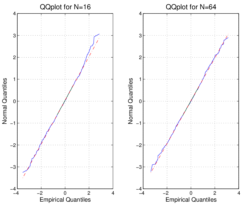
More precisely, Figure 4 quantifies this similarity through a Quantile-Quantile plot.

IV-B The separable case

In order to test the results of Proposition 2 and Corollary 1, we consider the following multiple antenna (MIMO) model with exponentially decaying correlation at reception:

{\boldsymbol{\Sigma}}=\frac{1}{\sqrt{K}}{\boldsymbol{\Psi}}^{1/2}{\bf W}{\bf P}^{1/2}

where ${\boldsymbol{\Psi}}=\left[a^{m-n}\right]_{m,n=0}^{N-1}$ with $0<a<1$ is the covariance matrix that accounts for the correlations at the receiver side, $P=\mbox{diag}\left(p_{0},\cdots,p_{K}\right)$ is the matrix of the powers given to the different sources and $W$ is a $N\times(K+1)$ matrix with Gaussian standard iid elements. Let $\bf{P_{u}}$ denote the vector containing the powers of the interfering sources. We set $\bf{P_{u}}$ (up to a permutation of its elements) to:

\bf{P_{u}}=\left\{\begin{array}[]{l}\left[4P\ \ 5P\right]\ \ \ \mathrm{if}\ \ K=2\\ \left[P\ \ P\ \ 2P\ \ 4P\right]\ \ \ \mathrm{if}\ \ K=4\\ \left[P\ \ P\ \ 2P\ \ 2P\ \ 2P\ \ 4P\ \ 4P\ \ 4P\ \ 8P\ \ 16P\ \ 16P\ \ 16P\ \right]\ \mathrm{if}\ K=12\ .\\ \end{array}\right.

For $K=2^{p}$ with $3\leq p\leq 7$ , we assume that the powers of the interfering sources are arranged into $5$ classes as in Table I. We set the SNR $P/\rho$ to $10$ dB and $a$ to $0.1$ . We investigate in this section the accuracy of the Gaussian approximation in terms of the outage probability. In Fig.5, we compare the empirical $1\%$ outage SINR with the one predicted by the Central Limit Theorem. We note that the Gaussian approximation tends to under estimate the $1$ % outage SINR. We also note that it has a good accuracy for small values of $\alpha$ and for enough large values of $N$ ( $N\geq 64$ ).

Observe that all these simulations confirm a fact announced in Remark 2 above: compared with functionals of the channel singular values such as Shannon’s mutual information, larger signal dimensions are needed to attain the asymptotic regime for quadratic forms such as the SINR (see for instance outage probability approximations for mutual information in [22] and in [23]). This observation holds for first order as well as for second order results.

V Proof of Theorem 3

This section is devoted to the proof of Theorem 3. We begin with mathematical preliminaries.

V-A Preliminaries

The following lemma gathers useful matrix results, whose proofs can be found in [28]:

Lemma 2

Assume ${\bf X}=[x_{ij}]_{i,j=1}^{N}$ and ${\bf Y}$ are complex $N\times N$ matrices. Then

1.

For every $i,j\leq N$ , $|x_{ij}|\leq\|{\bf X}\|$ . In particular, $\|{\mathrm{diag}}({\bf X})\|\leq\|{\bf X}\|$ .
2.

$\|{\bf XY}\|\leq\|{\bf X}\|\,\|{\bf Y}\|$ .
3.

For $\rho>0$ , the resolvent $({\bf XX}^{*}+\rho{\bf I})^{-1}$ satisfies $\|({\bf XX}^{*}+\rho{\bf I})^{-1}\|\leq\rho^{-1}$ .
4.

If ${\bf Y}$ is Hermitian nonnegative, then $|{\mathrm{tr}}({\bf XY})|\leq\|{\bf X}\|{\mathrm{tr}}({\bf Y})$ .

Let ${\bf X}={\bf U}{\boldsymbol{\Lambda}}{\bf V}^{*}$ be a spectral decomposition of ${\bf X}$ where ${\boldsymbol{\Lambda}}={\mathrm{diag}}(\lambda_{1},\ldots,\lambda_{n})$ is the matrix of singular values of ${\bf X}$ . For a real $p\geq 1$ , the Schatten $\ell_{p}$ -norm of ${\bf X}$ is defined as $\|{\bf X}\|_{p}=\left(\sum\lambda_{i}^{p}\right)^{1/p}$ . The following bound over the Schatten $\ell_{p}$ -norm of a triangular matrix will be of help (for a proof, see [25], [29, page 278]):

Lemma 3

Let ${\bf X}=[x_{ij}]_{i,j=1}^{N}$ be a $N\times N$ complex matrix and let $\widetilde{\bf X}=[x_{ij}{\bf 1}_{i>j}]_{i,j=1}^{N}$ be the strictly lower triangular matrix extracted from ${\bf X}$ . Then for every $p\geq 1$ , there exists a constant $C_{p}$ depending on $p$ only such that

\|\widetilde{\bf X}\|_{p}\leq C_{p}\|{\bf X}\|_{p}\ .

The following lemma lists some properties of the resolvent ${\bf Q}$ and the deterministic approximation matrix ${\bf T}$ . Its proof is postponed to Appendix -D.

Lemma 4

The following facts hold true:

1.

Assume A2. Consider matrices ${\bf T}_{K}(-\rho)={\mathrm{diag}}(t_{1}(-\rho),\ldots,t_{N}(-\rho))$ defined by Theorem 1–(1). Then for every $1\leq n\leq N$ ,

$\frac{1}{\rho+\sigma_{\max}^{2}}\leq t_{n}(-\rho)\leq\frac{1}{\rho}\ .$ (23)
2.

Assume in addition A1 and A3. Let ${\bf Q}_{K}(-\rho)=({\bf YY}^{*}+\rho{\bf I})^{-1}$ and let matrices ${\bf S}_{K}$ be as in the statement of Theorem 1–(2). Then

$\sup_{K}{\mathbb{E}}\left|{\mathrm{tr}}\ {\bf S}_{K}({\bf Q}_{K}-{\bf T}_{K})\right|^{2}<\infty\ .$ (24)

V-B Proof of Theorem 3–(1)

We introduce the following notations. Assume that ${\bf X}$ is a real matrix, by ${\bf X}\succcurlyeq{\bf 0}$ we mean $X_{ij}\geq 0$ for every element $X_{ij}$ . For a vector ${\bf x}$ , ${\bf x}\succcurlyeq{\bf 0}$ is defined similarly. In the remainder of the paper, $C=C(\rho,\sigma_{\max}^{2},\liminf\frac{N}{K},\sup\frac{N}{K})<\infty$ denotes a positive constant whose value may change from line to line.

The following lemma, which directly follows from [21, Lemma 5.2 and Proposition 5.5], states some important properties of the matrices ${\bf A}_{K}$ defined in the statement of Theorem 3.

Lemma 5

Assume A2 and A3. Consider matrices ${\bf A}_{K}$ defined by (19). Then the following facts hold true:

1.

Matrix ${\bf I}_{K}-{\bf A}_{K}$ is invertible, and $({\bf I}_{K}-{\bf A}_{K})^{-1}\succcurlyeq{\bf 0}$ .
2.

Element $(k,k)$ of the inverse satisfies $\left[({\bf I}_{K}-{\bf A}_{K})^{-1}\right]_{k,k}\geq 1$ for every $1\leq k\leq K$ .
3.

The maximum row sum norm of the inverse satisfies $\limsup_{K}\left|\!\left|\!\left|({\bf I}_{K}-{\bf A}_{K})^{-1}\right|\!\right|\!\right|_{\infty}<\infty$ .

Due to Lemma 5–(1), $\Theta_{K}^{2}$ is well defined. Let us prove that $\limsup_{K}\Theta_{K}^{2}<\infty$ . The first term of the right-hand side of (20) satisfies

\frac{1}{K}{\bf g}^{\mathrm{T}}({\bf I}_{K}-{\bf A}_{K})^{-1}{\boldsymbol{\Delta}}^{-1}{\bf g}\leq\|{\bf g}\|_{\infty}\|({\bf I}_{K}-{\bf A}_{K})^{-1}{\boldsymbol{\Delta}}^{-1}{\bf g}\|_{\infty}\\ \leq\|{\bf g}\|_{\infty}\left|\!\left|\!\left|({\bf I}_{K}-{\bf A}_{K})^{-1}\right|\!\right|\!\right|_{\infty}\|{\boldsymbol{\Delta}}^{-1}{\bf g}\|_{\infty}\leq\|{\bf g}\|_{\infty}^{2}\left|\!\left|\!\left|({\bf I}_{K}-{\bf A}_{K})^{-1}\right|\!\right|\!\right|_{\infty}

(25)

due to $\left|\!\left|\!\left|{\boldsymbol{\Delta}}^{-1}\right|\!\right|\!\right|_{\infty}\leq 1$ . Recall that $\|{\bf T}\|\leq\rho^{-1}$ by Lemma 4–(1). Therefore, any element of ${\bf g}$ satisfies

\frac{1}{K}{\mathrm{tr}}{\bf D}_{0}{\bf D}_{k}{\bf T}^{2}\leq\frac{N}{K}\|{\bf D}_{0}\|\|{\bf D}_{k}\|\|{\bf T}\|^{2}\leq\frac{N}{K}\frac{\sigma_{\max}^{4}}{\rho^{2}}

(26)

by A2, hence $\sup_{K}\|{\bf g}\|\leq C$ . From Lemma 5–(3) and (25), we then obtain

\limsup_{K}\frac{1}{K}{\bf g}^{\mathrm{T}}({\bf I}_{K}-{\bf A}_{K})^{-1}{\boldsymbol{\Delta}}^{-1}{\bf g}\leq C.

(27)

We can prove similarly that the second term in the right-hand side of (20) satisfies $\sup_{K}(({\mathbb{E}}|W_{10}|^{4}-1)\frac{1}{K}{\mathrm{tr}}{\bf D}_{0}^{2}{\bf T}(-\rho)^{2})\leq C$ . Hence $\limsup_{K}\Theta_{K}^{2}<\infty$ .
Let us prove that $\liminf_{K}\Theta_{K}^{2}>0$ . We have

$\displaystyle\frac{1}{K}{\bf g}^{\mathrm{T}}({\bf I}_{K}-{\bf A}_{K})^{-1}{\boldsymbol{\Delta}}^{-1}{\bf g}$	$\displaystyle\stackrel{{\scriptstyle(a)}}{{\geq}}$	$\displaystyle\frac{1}{K}{\bf g}^{\mathrm{T}}{\mathrm{diag}}\left(({\bf I}_{K}-{\bf A}_{K})^{-1}\right){\boldsymbol{\Delta}}^{-1}{\bf g}$
	$\displaystyle\stackrel{{\scriptstyle(b)}}{{\geq}}$	$\displaystyle\frac{1}{\left(1+\frac{N}{K}\frac{\sigma_{\max}^{2}}{\rho}\right)^{2}}\frac{1}{K}\sum_{k=1}^{K}\left(\frac{1}{K}{\mathrm{tr}}{\bf D}_{0}{\bf D}_{k}{\bf T}^{2}\right)^{2}$
	$\displaystyle\stackrel{{\scriptstyle(c)}}{{\geq}}$	$\displaystyle\frac{1}{\left(1+\frac{N}{K}\frac{\sigma_{\max}^{2}}{\rho}\right)^{2}}\left(\frac{1}{K^{2}}{\mathrm{tr}}\ {\bf D}_{0}\left(\sum_{k=1}^{K}{\bf D}_{k}\right){\bf T}^{2}\right)^{2}$
	$\displaystyle\stackrel{{\scriptstyle(d)}}{{\geq}}$	$\displaystyle\frac{1}{\left(1+\frac{N}{K}\frac{\sigma_{\max}^{2}}{\rho}\right)^{2}(\rho+\sigma^{2}_{\max})^{4}}\left(\frac{1}{K^{2}}{\mathrm{tr}}\ {\bf D}_{0}\sum_{k=1}^{K}{\bf D}_{k}\right)^{2}$
	$\displaystyle\geq$	$\displaystyle{C}\left(\frac{1}{K^{2}}{\mathrm{tr}}\ {\bf D}_{0}\sum_{k=1}^{K}{\bf D}_{k}\right)^{2}\ ,$

where $(a)$ follows from the fact that $({\bf I}_{K}-{\bf A}_{K})^{-1}\succcurlyeq{\bf 0}$ (Lemma 5–(1), and the straightforward inequalities ${\boldsymbol{\Delta}}^{-1}\succcurlyeq{\bf 0}$ and ${\bf g}\succcurlyeq{\bf 0}$ ), $(b)$ follows from Lemma 5–(2) and $\|{\boldsymbol{\Delta}}\|\leq(1+\frac{N}{K}\frac{\sigma_{\max}^{2}}{\rho})^{2}$ , $(c)$ follows from the elementary inequality $n^{-1}\sum x_{i}^{2}\geq(n^{-1}\sum x_{i})^{2}$ , and $(d)$ is due to Lemma 4–(1). Similar derivations yield:

({\mathbb{E}}|W_{10}|^{4}-1)\frac{1}{K}{\mathrm{tr}}{\bf D}_{0}^{2}{\bf T}\quad\geq\quad\frac{{\mathbb{E}}|W_{10}|^{4}-1}{(\rho+\sigma_{\max}^{2})^{2}}\left(\frac{1}{K}{\mathrm{tr}}{\bf D}_{0}\right)^{2}\quad\geq\quad C({\mathbb{E}}|W_{10}|^{4}-1)

by A3. Therefore, if A4 holds true, then $\liminf_{K}\Theta_{K}^{2}>0$ and Theorem 3–(1) is proved.

V-C Proof of Theorem 3–(2)

Recall that the SINR $\beta_{K}$ is given by Equation (14). The random variable $\frac{\sqrt{K}}{\Theta_{K}}(\beta_{K}-\overline{\beta}_{K})$ can therefore be decomposed as

	$\displaystyle\frac{\sqrt{K}}{\Theta_{K}}(\beta_{K}-\overline{\beta}_{K})$	$\displaystyle=$	$\displaystyle\frac{1}{\sqrt{K}\Theta_{K}}\left({\bf w}_{0}^{*}{\bf D}_{0}^{1/2}{\bf Q}{\bf D}_{0}^{1/2}{\bf w}_{0}-{\mathrm{tr}}({\bf D}_{0}{\bf Q})\right)+\frac{1}{\sqrt{K}\Theta_{K}}\left({\mathrm{tr}}({\bf D}_{0}({\bf Q}-{\bf T}))\right)$		(28)
		$\displaystyle=$	$\displaystyle U_{1,K}+U_{2,K}\ .$		(28)

Thanks to Lemma 4–(2) and to the fact that $\liminf_{K}\Theta_{K}^{2}>0$ , we have ${\mathbb{E}}U_{K,2}^{2}<CK^{-1}$ which implies that $U_{K,2}\rightarrow 0$ in probability as ${K\rightarrow\infty}$ . Hence, in order to conclude that

\frac{\sqrt{K}}{\Theta_{K}}(\beta_{K}-\overline{\beta}_{K})\xrightarrow[K\to\infty]{}{\mathcal{N}}(0,1)\quad\text{in distribution}\ ,

it is sufficient by Slutsky’s theorem to prove that $U_{1,K}\to{\cal N}(0,1)$ in distribution. The remainder of the section is devoted to this point.

Remark 6

Decomposition (28) and the convergence to zero (in probability) of $U_{2,K}$ yield the following interpretation: The fluctuations of $\sqrt{K}(\beta_{K}-\overline{\beta}_{K})$ are mainly due to the fluctuations of vector ${\bf w}_{0}$ . Indeed the contribution of the fluctuations¹¹ 1 In fact, one may prove that the fluctuation of $\frac{1}{K}{\mathrm{tr}}{\bf D}_{0}({\bf Q}-{\bf T})$ are of order $K$ , i.e. ${\mathrm{tr}}{\bf D}_{0}({\bf Q}-{\bf T})$ asymptotically behaves as a Gaussian random variable. Such a speed of fluctuations already appears in [21], when studying the fluctuations of the mutual information. of $\frac{1}{K}{\mathrm{tr}}{\bf D}_{0}{\bf Q}$ , due to the random nature of ${\bf Y}$ , is negligible.

Denote by ${\mathbb{E}}_{n}$ the conditional expectation ${\mathbb{E}}_{n}[\ \cdot\ ]={\mathbb{E}}[\ \cdot\ \|\ W_{n,0},W_{n+1,0},\ldots,W_{N,0},{\bf Y}]$ . Put ${\mathbb{E}}_{N+1}[\ \cdot\ ]={\mathbb{E}}[\ \cdot\ \|\ {\bf Y}]$ and note that ${\mathbb{E}}_{N+1}({\bf w}_{0}^{*}{\bf D}_{0}^{1/2}{\bf Q}{\bf D}_{0}^{1/2}{\bf w}_{0})={\mathrm{tr}}{\bf D}_{0}{\bf Q}$ . With these notations at hand, we have:

U_{1,K}=\frac{1}{\Theta_{K}}\sum_{n=1}^{N}({\mathbb{E}}_{n}-{\mathbb{E}}_{n+1})\frac{{\bf w}_{0}^{*}{\bf D}_{0}^{1/2}{\bf Q}{\bf D}_{0}^{1/2}{\bf w}_{0}}{\sqrt{K}}\stackrel{{\scriptstyle\triangle}}{{=}}\frac{1}{\Theta_{K}}\sum_{n=1}^{N}Z_{n,K}\ .

(29)

Consider the increasing sequence of $\sigma-$ fields

{\cal F}_{N,K}=\sigma(W_{N,0},{\bf Y})\ ,\quad\cdots\ ,\quad{\cal F}_{1,K}=\sigma(W_{1,0},\cdots,W_{N,0},{\bf Y})\ .

Then the random variable $Z_{n,K}$ is integrable and measurable with respect to ${\cal F}_{n,K}$ ; moreover it readily satisfies ${\mathbb{E}}_{n+1}Z_{n,K}=0$ . In particular, the sequence $(Z_{N,K},\ldots,Z_{1,K})$ is a martingale difference sequence with respect to $\left({\cal F}_{N,K},\cdots,{\cal F}_{1,K}\right)$ . The following CLT for martingales is the key tool to study the asymptotic behavior of $U_{1,K}$ :

Theorem 4

Let $X_{N,K},X_{N-1,K},\ldots,X_{1,K}$ be a martingale difference sequence with respect to the increasing filtration ${\mathcal{G}}_{N,K},\ldots,{\mathcal{G}}_{1,K}$ . Assume that there exists a sequence of real positive numbers $s_{K}^{2}$ such that

\frac{1}{s_{K}^{2}}\sum_{n=1}^{N}{\mathbb{E}}\left[X_{n,K}^{2}\|{\mathcal{G}}_{n+1,K}\right]\xrightarrow[K\to\infty]{}1

in probability. Assume further that the Lyapunov condition holds:

\exists\alpha>0,\quad\frac{1}{s_{K}^{2(1+\alpha)}}\sum_{n=1}^{N}{\mathbb{E}}\left|X_{n,K}\right|^{2+\alpha}\xrightarrow[K\rightarrow\infty]{}0\ ,

Then $s_{K}^{-1}\sum_{n=1}^{N}X_{n,K}$ converges in distribution to ${\mathcal{N}}(0,1)$ as $K\to\infty$ .

Remark 7

This theorem is proved in [24], gathering Theorem 35.12 (which is expressed under the weaker Lindeberg condition) together with the arguments of Section 27 (where it is proved that Lyapunov’s condition implies Lindeberg’s condition).

In order to prove that

U_{1,K}=\frac{1}{\Theta_{K}}\sum_{n=1}^{N}Z_{n,K}\xrightarrow[K\to\infty]{}{\cal N}(0,1)\quad\text{in distribution}\ ,

(30)

we shall apply Theorem 4 to the sum $\frac{1}{\Theta_{K}}\sum_{n=1}^{N}Z_{n,K}$ and the filtration $\left({\cal F}_{n,K}\right)$ . The proof is carried out into four steps:

Step 1

We first establish Lyapunov’s condition. Due to the fact that $\liminf_{K}\Theta_{K}^{2}>0$ , we only need to show that

\exists\ \alpha>0,\quad\sum_{n=1}^{N}{\mathbb{E}}|Z_{n,K}|^{2+\alpha}\xrightarrow[K\to\infty]{}0\ .

(31)

Step 2

We prove that $V_{K}=\sum_{n=1}^{N}{\mathbb{E}}_{n+1}Z_{n,K}^{2}$ satisfies

V_{K}-\left(\frac{\left({\mathbb{E}}|W_{10}|^{4}-2\right)}{K}{\mathrm{tr}}\left({\bf D}_{0}^{2}({\mathrm{diag}}({\bf Q}))^{2}\right)+\frac{1}{K}{\mathrm{tr}}({\bf D}_{0}{\bf QD}_{0}{\bf Q})\right)\xrightarrow[K\to\infty]{}0\quad\text{in probability}\ .

(32)

Step 3

We first show that

\frac{1}{K}{\mathrm{tr}}{\bf D}_{0}^{2}({\mathrm{diag}}({\bf Q}))^{2}-\frac{1}{K}{\mathrm{tr}}{\bf D}_{0}^{2}{\bf T}^{2}\xrightarrow[K\to\infty]{}0\quad\text{in probability.}

(33)

In order to study the asymptotic behavior of $\frac{1}{K}{\mathrm{tr}}({\bf D}_{0}{\bf QD}_{0}{\bf Q})$ , we introduce the random variables $U_{\ell}=\frac{1}{K}{\mathrm{tr}}({\bf D}_{0}{\bf QD}_{\ell}{\bf Q})$ for $0\leq\ell\leq K$ (the one of interest being $U_{0}$ ). We then prove that the $U_{\ell}$ ’s satisfy the following system of equations:

U_{\ell}=\sum_{k=1}^{K}c_{\ell k}U_{k}+\frac{1}{K}{\mathrm{tr}}{\bf D}_{0}{\bf D}_{\ell}{\bf T}^{2}+\epsilon_{\ell},\quad 0\leq\ell\leq K,

(34)

where

c_{\ell k}=\frac{1}{K}\frac{\frac{1}{K}{\mathrm{tr}}{\bf D}_{\ell}{\bf D}_{k}{\bf T}(-\rho)^{2}}{\left(1+\frac{1}{K}{\mathrm{tr}}{\bf D}_{k}{\bf T}(-\rho)\right)^{2}},\quad 0\leq\ell\leq K,\ 1\leq k\leq K

(35)

and the perturbations $\epsilon_{\ell}$ satisfy ${\mathbb{E}}|\epsilon_{\ell}|\leq CK^{-\frac{1}{2}}$ where we recall that $C$ is independent of $\ell$ .

Step 4

We prove that $U_{0}=\frac{1}{K}{\mathrm{tr}}{\bf D}_{0}{\bf Q}{\bf D}_{0}{\bf Q}$ satisfies

U_{0}=\frac{1}{K}{\mathrm{tr}}{\bf D}_{0}^{2}{\bf T}^{2}+\frac{1}{K}{\bf g}^{\mathrm{T}}\left({\bf I}-{\bf A}\right)^{-1}{\boldsymbol{\Delta}}^{-1}{\bf g}+\epsilon

(36)

with ${\mathbb{E}}|\epsilon|\leq CK^{-\frac{1}{2}}$ . This equation combined with (32) and (33) yields $\sum_{n}{\mathbb{E}}_{n+1}Z_{n,K}^{2}-\Theta_{K}^{2}\to 0$ in probability. As $\liminf_{K}\Theta_{K}^{2}>0$ , this implies $\frac{1}{\Theta_{K}}\sum_{n}{\mathbb{E}}_{n+1}Z_{n,K}^{2}\to 1$ in probability, which proves (30) and thus ends the proof of Theorem 3.

Write ${\bf B}=[b_{ij}]_{i,j=1}^{N}={\bf D}_{0}^{1/2}{\bf Q}{\bf D}_{0}^{1/2}$ and recall from (29) that $Z_{n,K}=\frac{1}{\sqrt{K}}({\mathbb{E}}_{n}-{\mathbb{E}}_{n+1}){\bf w}_{0}^{*}{\bf B}{\bf w}_{0}$ . We have

{\mathbb{E}}_{n}{\bf w}_{0}^{*}{\bf B}{\bf w}_{0}=\sum_{\ell=1}^{n-1}b_{\ell\ell}+\sum_{\ell_{1},\ell_{2}=n}^{N}W_{\ell_{1}0}^{*}W_{\ell_{2}0}b_{\ell_{1}\ell_{2}}\ .

Hence

Z_{n,K}=\frac{1}{\sqrt{K}}\left(\left(|W_{n0}|^{2}-1\right)b_{nn}+W_{n0}^{*}\sum_{\ell=n+1}^{N}W_{\ell 0}b_{n\ell}+W_{n0}\sum_{\ell=n+1}^{N}W_{\ell 0}^{*}b_{\ell n}\right)\ .

(37)

Step 1: Validation of the Lyapunov condition

The following inequality will be of help to check Lyapunov’s condition.

Lemma 6 (Burkholder’s inequality)

Let $X_{k}$ be a complex martingale difference sequence with respect to the increasing sequence of $\sigma$ –fields ${\cal F}_{k}$ . Then for $p\geq 2$ , there exists a constant $C_{p}$ for which

{\mathbb{E}}\left|\sum_{k}X_{k}\right|^{p}\leq C_{p}\left({\mathbb{E}}\left(\sum_{k}{\mathbb{E}}\left[|X_{k}|^{2}\|{\cal F}_{k-1}\right]\right)^{p/2}+{\mathbb{E}}\sum_{k}|X_{k}|^{p}\right)\ .

Recall Assumption A1. Eq. (37) yields:

	$\displaystyle\left\|Z_{n,K}\right\|^{4}$	$\displaystyle\leq$	$\displaystyle\frac{1}{K^{2}}\left(\frac{\|W_{n0}\|^{2}+1}{\rho\sigma_{\max}^{2}}+2\left\|W_{n0}\sum_{\ell=n+1}^{N}W_{\ell 0}b_{n\ell}\right\|\right)^{4}$		(38)
		$\displaystyle\leq$	$\displaystyle\frac{2^{3}}{K^{2}}\left(\left(\frac{\|W_{n0}\|^{2}+1}{\rho\sigma_{\max}^{2}}\right)^{4}+2^{4}\left\|W_{n0}\sum_{\ell=n+1}^{N}W_{\ell 0}b_{n\ell}\right\|^{4}\right)$		(38)

where we use the fact that $|b_{nn}|\leq(\rho\sigma^{2}_{\max})^{-1}$ (cf. Lemma 2–(1)) and the convexity of $x\mapsto x^{4}$ . Due to Assumption A1, we have:

{\mathbb{E}}\left(|W_{n0}|^{2}+1\right)^{4}\leq 2^{3}\left({\mathbb{E}}|W_{n0}|^{8}+1\right)<\infty\ .

(39)

Considering the second term at the right-hand side of (38), we write

$\displaystyle{\mathbb{E}}\left\|W_{n0}\sum_{\ell=n+1}^{N}W_{\ell 0}b_{n\ell}\right\|^{4}$	$\displaystyle=$	$\displaystyle{\mathbb{E}}\left\|W_{n0}\right\|^{4}{\mathbb{E}}\left\|\sum_{\ell=n+1}^{N}W_{\ell 0}b_{n\ell}\right\|^{4}\ ,$
	$\displaystyle\stackrel{{\scriptstyle(a)}}{{\leq}}$	$\displaystyle C\left({\mathbb{E}}\left(\sum_{\ell=n+1}^{N}({\mathbb{E}}\|W_{\ell 0}\|^{2})\|b_{n\ell}\|^{2}\right)^{2}+\sum_{\ell=n+1}^{N}({\mathbb{E}}\|W_{\ell 0}\|^{4})({\mathbb{E}}\|b_{n\ell}\|^{4})\right)\ ,$
	$\displaystyle\stackrel{{\scriptstyle(b)}}{{\leq}}$	$\displaystyle C\left({\mathbb{E}}\left(\sum_{\ell=n+1}^{N}\|b_{n\ell}\|^{2}\right)^{2}+\sum_{\ell=n+1}^{N}{\mathbb{E}}\|b_{n\ell}\|^{2}\right)\ ,$

where $(a)$ follows from Lemma 6 (Burkholder’s inequality), the filtration being ${\cal F}_{N,K},\ldots,$ ${\cal F}_{n+1,K}$ and $(b)$ follows from the bound $|b_{n\ell}|^{4}\leq|b_{n\ell}|^{2}\max\,|b_{n\ell}|^{2}\leq|b_{n\ell}|^{2}(\sigma^{2}_{\max}\rho^{-1})^{2}$ (cf. Lemma 2–(1)). Now, notice that

\sum_{\ell=n+1}^{N}|b_{n\ell}|^{2}<\sum_{\ell=1}^{N}|b_{n\ell}|^{2}=\left[{\bf D}_{0}^{1/2}{\bf Q}{\bf D}_{0}{\bf Q}{\bf D}_{0}^{1/2}\right]_{nn}\leq\|{\bf D}_{0}^{1/2}{\bf Q}{\bf D}_{0}{\bf Q}{\bf D}_{0}^{1/2}\|\leq\frac{\sigma_{\max}^{4}}{\rho^{2}}\ .

This yields ${\mathbb{E}}|W_{n0}\sum_{\ell=n+1}^{N}W_{\ell\,0}b_{n\ell}|^{4}\leq C$ . Gathering this result with (39), getting back to (38), taking the expectation and summing up finally yields:

\sum_{n=1}^{N}{\mathbb{E}}|Z_{n,K}|^{4}\ \leq\ \frac{C}{K}\ \xrightarrow[K\to\infty]{}\ 0

which establishes Lyapunov’s condition (31) with $\alpha=2$ .

Step 2: Proof of (32)

Eq. (37) yields:

	$\displaystyle{\mathbb{E}}_{n+1}Z_{n,K}^{2}$	$\displaystyle=$	$\displaystyle\frac{1}{K}\left(\phantom{\sum_{\ell=n+1}^{N}}\!\!\!\!\!\!\!\!\!\!\!\!\!\!\!\!\!\right.\left({\mathbb{E}}\|W_{10}\|^{4}-1\right)b_{nn}^{2}+{\mathbb{E}}_{n+1}\left(W_{n0}^{}\sum_{\ell=n+1}^{N}W_{\ell 0}b_{n\ell}+W_{n0}\sum_{\ell=n+1}^{N}W_{\ell 0}^{}b_{\ell n}\right)^{2}$
			$\displaystyle+2b_{nn}\left({\mathbb{E}}\,W_{10}^{}\|W_{10}\|^{2}\right)\sum_{\ell=n+1}^{N}W_{\ell 0}b_{n\ell}+2b_{nn}\left({\mathbb{E}}\,W_{10}\|W_{10}\|^{2}\right)\sum_{\ell=n+1}^{N}W_{\ell 0}^{}b_{\ell n}\left.\phantom{\sum_{\ell=n+1}^{N}}\!\!\!\!\!\!\!\!\!\!\!\!\!\!\!\!\!\!\right)\ .$

Note that the second term of the right-hand side writes:

{\mathbb{E}}_{n+1}\left(W_{n0}^{*}\sum_{\ell=n+1}^{N}W_{\ell 0}b_{n\ell}+W_{n0}\sum_{\ell=n+1}^{N}W_{\ell 0}^{*}b_{\ell n}\right)^{2}=2\sum_{\ell_{1},\ell_{2}=n+1}^{N}W_{\ell_{1}0}W_{\ell_{2}0}^{*}b_{n\ell_{1}}b_{\ell_{2}n}\ .

Therefore, $V_{K}=\sum_{n=1}^{N}{\mathbb{E}}_{n+1}Z_{n,K}^{2}$ writes:

V_{K}=\frac{\left({\mathbb{E}}|W_{10}|^{4}-1\right)}{K}\sum_{n=1}^{N}b_{nn}^{2}+\frac{2}{K}\sum_{n=1}^{N}\sum_{\ell_{1},\ell_{2}=n+1}^{N}W_{\ell_{1}0}W_{\ell_{2}0}^{*}b_{n\ell_{1}}b_{\ell_{2}n}\\ +\frac{2}{K}\Re\left(\left({\mathbb{E}}\,W_{10}^{*}|W_{10}|^{2}\right)\sum_{n=1}^{N}b_{nn}\sum_{\ell=n+1}^{N}W_{\ell 0}b_{n\ell}\right)\ ,

where $\Re$ denotes the real part of a complex number. We introduce the following notations:

{\bf R}=\left(r_{ij}\right)_{i,j=1}^{N}\stackrel{{\scriptstyle\triangle}}{{=}}\left(b_{ij}{\bf 1}_{i>j}\right)_{i,j=1}^{N}\qquad\textrm{and}\qquad\Gamma_{K}=\frac{1}{K}\sum_{n=1}^{N}b_{nn}\sum_{\ell=n+1}^{N}W_{\ell 0}b_{n\ell}\ .

Note in particular that ${\bf R}$ is the strictly lower triangular matrix extracted from ${\bf D}_{0}^{1/2}{\bf Q}{\bf D}_{0}^{1/2}$ . We can now rewrite $V_{K}$ as:

V_{K}=\frac{\left({\mathbb{E}}|W_{10}|^{4}-1\right)}{K}{\mathrm{tr}}\left({\bf D}_{0}^{2}({\mathrm{diag}}({\bf Q}))^{2}\right)+\frac{2}{K}{\bf w}_{0}^{*}{\bf RR}^{*}{\bf w}_{0}+2\Re\left(\Gamma_{K}{\mathbb{E}}W_{10}^{*}|W_{10}|^{2}\right)\ .

(40)

We now prove that the third term of the right-hand side vanishes, and find an asymptotic equivalent for the second one. Using Lemma 2, we have:

$\displaystyle{\mathbb{E}}_{N+1}\|\Gamma_{K}\|^{2}$	$\displaystyle=$	$\displaystyle\frac{1}{K^{2}}\sum_{n,m=1}^{N}b_{nn}b_{mm}\sum_{\ell=1}^{N}b_{n\ell}b_{m\ell}^{}{\bf 1}_{\ell>n}{\bf 1}_{\ell>m}=\frac{1}{K^{2}}{\mathrm{tr}}\left({\mathrm{diag}}({\bf B}){\bf R}^{}{\bf R}{\mathrm{diag}}({\bf B})\right)$
	$\displaystyle=$	$\displaystyle\frac{1}{K^{2}}{\mathrm{tr}}\left({\bf D}_{0}^{1/2}{\mathrm{diag}}({\bf Q}){\bf D}_{0}^{1/2}{\bf R}^{*}{\bf R}{\bf D}_{0}^{1/2}{\mathrm{diag}}({\bf Q}){\bf D}_{0}^{1/2}\right)$
	$\displaystyle\leq$	$\displaystyle\frac{1}{K^{2}}\\|{\bf D}_{0}\\|^{2}\\|{\bf Q}\\|^{2}{\mathrm{tr}}({\bf R}^{*}{\bf R})\quad\leq\quad\frac{1}{K^{2}}\\|{\bf D}_{0}\\|^{2}\\|{\bf Q}\\|^{2}{\mathrm{tr}}({\bf B}^{2})\quad\leq\quad\frac{1}{K^{2}}\\|{\bf D}_{0}\\|^{4}\\|{\bf Q}\\|^{2}{\mathrm{tr}}({\bf Q}^{2})$
	$\displaystyle\leq$	$\displaystyle\frac{1}{K}\\|{\bf D}_{0}\\|^{2}\\|{\bf Q}\\|^{4}\quad\leq\quad\frac{1}{K}\frac{\sigma_{\max}^{4}}{\rho^{4}}\quad\xrightarrow[K\to\infty]{}\quad 0\ .$

In particular, ${\mathbb{E}}|\Gamma_{K}|^{2}\rightarrow 0$ and

\Re\left(\left({\mathbb{E}}W_{10}^{*}|W_{10}|^{2}\right)\Gamma_{K}\right)\xrightarrow[K\to\infty]{}0\quad\text{in probability}\ .

(41)

Consider now the second term of the right-hand side of Eq. (40). We prove that:

\frac{1}{K}{\bf w}_{0}^{*}{\bf RR}^{*}{\bf w}_{0}-\frac{1}{K}{\mathrm{tr}}({\bf RR}^{*})\xrightarrow[K\to\infty]{}0\quad\text{in probability.}

(42)

By Lemma 1 (Ineq. (12)), we have

{\mathbb{E}}\left(\frac{1}{K}{\bf w}_{0}^{*}{\bf RR}^{*}{\bf w}_{0}-\frac{1}{K}{\mathrm{tr}}({\bf RR}^{*})\right)^{2}\leq\frac{C}{K^{2}}({\mathbb{E}}|W_{10}|^{4}){\mathrm{tr}}({\bf RR}^{*}{\bf RR}^{*})\ .

Notice that ${\mathrm{tr}}({\bf RR}^{*}{\bf RR}^{*})=\|{\bf R}\|_{4}^{4}$ where $\|{\bf R}\|_{4}$ is the Schatten $\ell_{4}$ -norm of ${\bf R}$ . Using Lemma 3, we have:

\|{\bf R}\|_{4}^{4}\leq C\|{\bf D}_{0}^{1/2}{\bf Q}{\bf D}_{0}^{1/2}\|_{4}^{4}\leq NC\|{\bf D}_{0}^{1/2}{\bf Q}{\bf D}_{0}^{1/2}\|^{4}\leq N\frac{C\sigma_{\max}^{8}}{\rho^{4}}\ .

Therefore,

{\mathbb{E}}\left(\frac{1}{K}{\bf w}_{0}^{*}{\bf RR}^{*}{\bf w}_{0}-\frac{1}{K}{\mathrm{tr}}({\bf RR}^{*})\right)^{2}\leq C\frac{N}{K^{2}}\xrightarrow[K\to\infty]{}0

which implies (42). Now, due to the fact that ${\bf B}={\bf B}^{*}$ , we have

$\displaystyle\frac{2}{K}{\mathrm{tr}}\,{\bf RR}^{*}$	$\displaystyle=$	$\displaystyle\frac{2}{K}\sum_{n=1}^{N}\sum_{\ell=n+1}^{N}\|b_{n\ell}\|^{2}$	(43)
	$\displaystyle=$	$\displaystyle\frac{1}{K}\sum_{n,\ell=1}^{N}\|b_{n\ell}\|^{2}-\frac{1}{K}\sum_{n=1}^{N}\|b_{nn}\|^{2}$
	$\displaystyle=$	$\displaystyle\frac{1}{K}{\mathrm{tr}}\,{\bf D}_{0}{\bf QD}_{0}{\bf Q}-\frac{1}{K}{\mathrm{tr}}\,{\bf D}_{0}^{2}({\mathrm{diag}}({\bf Q}))^{2}$

Gathering (40–43), we obtain (32). Step 2 is proved.

Step 3: Proof of (33) and (34)

We begin with some identities. Write ${\bf Q}(z)=[q_{ij}(z)]_{i,j=1}^{N}$ and $\widetilde{\bf Q}(z)=[\tilde{q}_{ij}(z)]_{i,j=1}^{K}$ . Denote by ${\bf y}_{k}$ the column number $k$ of ${\bf Y}$ and by ${\boldsymbol{\xi}}_{n}$ the row number $n$ of ${\bf Y}$ . Denote by ${\bf Y}^{k}$ the matrix that remains after deleting column $k$ from ${\bf Y}$ and by ${\bf Y}_{n}$ the matrix that remains after deleting row $n$ from ${\bf Y}$ . Finally, write ${\bf Q}_{k}(z)=({\bf Y}^{k}{{\bf Y}^{k}}^{*}-z{\bf I})^{-1}$ and $\widetilde{\bf Q}_{n}(z)=({\bf Y}_{n}^{*}{\bf Y}_{n}-z{\bf I})^{-1}$ . The following formulas can be established easily (see for instance [28, §0.7.3. and §0.7.4]):

q_{nn}(-\rho)=\frac{1}{\rho(1+{\boldsymbol{\xi}}_{n}\widetilde{\bf Q}_{n}(-\rho){\boldsymbol{\xi}}_{n}^{*})},\quad\tilde{q}_{kk}(-\rho)=\frac{1}{\rho(1+{\bf y}_{k}^{*}{\bf Q}_{k}(-\rho){\bf y}_{k})},

(44)

{\bf Q}={\bf Q}_{k}-\frac{{\bf Q}_{k}{\bf y}_{k}{\bf y}_{k}^{*}{\bf Q}_{k}}{1+{\bf y}_{k}^{*}{\bf Q}_{k}{\bf y}_{k}}

(45)

Lemma 7

The following hold true:

1.

(Rank one perturbation inequality) The resolvent ${\bf Q}_{k}(-\rho)$ satisfies $\left|{\mathrm{tr}}{\bf A}({\bf Q}-{\bf Q}_{k})\right|\leq\|{\bf A}\|/\rho$ for any $N\times N$ matrix ${\bf A}$ .
2.

Let Assumptions A1–A3 hold. Then,

$\max_{1\leq n\leq N}{\mathbb{E}}(q_{nn}(-\rho)-t_{n}(-\rho))^{2}\leq\frac{C}{K}\ .$ (46)

The same conclusion holds true if $q_{nn}$ and $t_{n}$ are replaced with $\tilde{q}_{kk}$ and $\tilde{t}_{k}$ respectively.

We are now in position to prove (33). First, notice that:

	$\displaystyle{\mathbb{E}}\left\|q_{nn}^{2}-t_{n}^{2}\right\|$	$\displaystyle=$	$\displaystyle{\mathbb{E}}\left\|q_{nn}-t_{n}\right\|\left(q_{nn}+t_{n}\right)$		(47)
		$\displaystyle\leq$	$\displaystyle\sqrt{{\mathbb{E}}(q_{nn}-t_{n})^{2}}\sqrt{{\mathbb{E}}(q_{nn}+t_{n})^{2}}\quad\leq\quad\frac{2}{\rho}\sqrt{{\mathbb{E}}(q_{nn}-t_{n})^{2}}\ .$		(47)

Now,

	$\displaystyle\frac{1}{K}{\mathbb{E}}\left\|{\mathrm{tr}}\,{\bf D}_{0}^{2}({\mathrm{diag}}({\bf Q})^{2}-{\bf T}^{2})\right\|$	$\displaystyle\leq$	$\displaystyle\frac{1}{K}\sum_{n=1}^{N}\sigma_{0,n}^{4}{\mathbb{E}}\left\|q_{nn}^{2}-t_{n}^{2}\right\|\quad\leq\quad\frac{\sigma_{\max}^{4}N}{K}\max_{1\leq n\leq N}{\mathbb{E}}\left\|q_{nn}^{2}-t_{n}^{2}\right\|$
		$\displaystyle\leq$	$\displaystyle\frac{2\sigma_{\max}^{4}N}{\rho K}\sqrt{\max_{1\leq n\leq N}{\mathbb{E}}(q_{nn}-t_{n})^{2}}\quad\xrightarrow[K\rightarrow\infty]{}\quad 0\ ,$

where the last inequality follows from (47) together with Lemma 7–(2). Convergence (33) is established.

We now establish the system of equations (34). Our starting point is the identity

{\bf Q}={\bf T}+{\bf T}({\bf T}^{-1}-{\bf Q}^{-1}){\bf Q}={\bf T}+\frac{\rho}{K}{\bf T}\,{\mathrm{diag}}({\mathrm{tr}}\widetilde{\bf D}_{1}\widetilde{\bf T},\ldots,{\mathrm{tr}}\widetilde{\bf D}_{N}\widetilde{\bf T}){\bf Q}-{\bf T}{\bf YY}^{*}{\bf Q}\ .

Using this identity, we develop $U_{\ell}=\frac{1}{K}{\mathrm{tr}}{\bf D}_{0}{\bf Q}{\bf D}_{\ell}{\bf Q}$ as

	$\displaystyle U_{\ell}$	$\displaystyle=$	$\displaystyle\frac{1}{K}{\mathrm{tr}}{\bf D}_{0}{\bf QD}_{\ell}{\bf T}+\frac{\rho}{K^{2}}{\mathrm{tr}}{\bf D}_{0}{\bf QD}_{\ell}{\bf T}{\mathrm{diag}}({\mathrm{tr}}\widetilde{\bf D}_{1}\widetilde{\bf T},\ldots,{\mathrm{tr}}\widetilde{\bf D}_{N}\widetilde{\bf T}){\bf Q}-\frac{1}{K}{\mathrm{tr}}{\bf D}_{0}{\bf QD}_{\ell}{\bf T}{\bf YY}^{*}{\bf Q}$		(48)
		$\displaystyle\stackrel{{\scriptstyle\triangle}}{{=}}$	$\displaystyle X_{1}+X_{2}-X_{3}\ .$		(48)

Lemma 4–(2) with ${\bf S}={\bf D}_{0}{\bf D}_{\ell}{\bf T}$ yields:

X_{1}=\frac{1}{K}{\mathrm{tr}}{\bf D}_{0}{\bf D}_{\ell}{\bf T}^{2}+\epsilon_{1}

(49)

where ${\mathbb{E}}|\epsilon_{1}|\leq\sqrt{{\mathbb{E}}\epsilon_{1}^{2}}\leq C/K$ . Consider now the term $X_{3}=\frac{1}{K}\sum_{k=1}^{K}{\mathrm{tr}}{\bf D}_{0}{\bf QD}_{\ell}{\bf T}{\bf y}_{k}{\bf y}_{k}^{*}{\bf Q}$ . Using (44) and (45), we have

{\bf y}_{k}^{*}{\bf Q}=\left(1-\frac{{\bf y}_{k}^{*}{\bf Q}{\bf y}_{k}}{1+{\bf y}_{k}^{*}{\bf Q}{\bf y}_{k}}\right){\bf y}_{k}^{*}{\bf Q}_{k}=\rho\,\tilde{q}_{kk}\,{\bf y}_{k}^{*}{\bf Q}_{k}\ .

Hence

$\displaystyle X_{3}$	$\displaystyle=$	$\displaystyle\frac{\rho}{K}\sum_{k=1}^{K}\tilde{q}_{kk}{\bf y}_{k}^{*}{\bf Q}_{k}{\bf D}_{0}{\bf Q}{\bf D}_{\ell}{\bf T}{\bf y}_{k}$	(50)
	$\displaystyle=$	$\displaystyle\frac{\rho}{K}\sum_{k=1}^{K}\tilde{t}_{k}{\bf y}_{k}^{}{\bf Q}_{k}{\bf D}_{0}{\bf Q}{\bf D}_{\ell}{\bf T}{\bf y}_{k}+\frac{\rho}{K}\sum_{k=1}^{K}(\tilde{q}_{kk}-\tilde{t}_{k}){\bf y}_{k}^{}{\bf Q}_{k}{\bf D}_{0}{\bf Q}{\bf D}_{\ell}{\bf T}{\bf y}_{k}$
	$\displaystyle\stackrel{{\scriptstyle\triangle}}{{=}}$	$\displaystyle X^{\prime}_{3}+\epsilon_{2}\ .$

By Cauchy-Schwartz inequality,

{\mathbb{E}}|\epsilon_{2}|\leq\frac{\rho}{K}\sum_{k=1}^{K}\sqrt{{\mathbb{E}}(\tilde{q}_{kk}-\tilde{t}_{k})^{2}}\sqrt{{\mathbb{E}}({\bf y}_{k}^{*}{\bf Q}_{k}{\bf D}_{0}{\bf Q}{\bf D}_{\ell}{\bf T}{\bf y}_{k})^{2}}\ .

We have ${\mathbb{E}}({\bf y}_{k}^{*}{\bf Q}_{k}{\bf D}_{0}{\bf Q}{\bf D}_{\ell}{\bf T}{\bf y}_{k})^{2}\leq\sigma_{\max}^{8}\rho^{-6}{\mathbb{E}}\|{\bf y}_{k}\|^{4}\leq C$ . Using in addition Lemma 7–(2), we obtain

{\mathbb{E}}|\epsilon_{2}|\leq\frac{C}{\sqrt{K}}\ .

Consider $X^{\prime}_{3}$ . From (44) and (45), we have ${\bf Q}={\bf Q}_{k}-\rho\tilde{q}_{kk}{\bf Q}_{k}{\bf y}_{k}{\bf y}_{k}^{*}{\bf Q}_{k}$ . Hence, we can develop $X^{\prime}_{3}$ as

	$\displaystyle X^{\prime}_{3}$	$\displaystyle=$	$\displaystyle\frac{\rho}{K}\sum_{k=1}^{K}\tilde{t}_{k}{\bf y}_{k}^{}{\bf Q}_{k}{\bf D}_{0}{\bf Q}_{k}{\bf D}_{\ell}{\bf T}{\bf y}_{k}-\frac{\rho^{2}}{K}\sum_{k=1}^{K}\tilde{t}_{k}\tilde{q}_{kk}{\bf y}_{k}^{}{\bf Q}_{k}{\bf D}_{0}{\bf Q}_{k}{\bf y}_{k}{\bf y}_{k}^{*}{\bf Q}_{k}{\bf D}_{\ell}{\bf T}{\bf y}_{k}$		(51)
		$\displaystyle\stackrel{{\scriptstyle\triangle}}{{=}}$	$\displaystyle X_{4}+X_{5}\ .$		(51)

Consider $X_{4}$ . Notice that ${\bf y}_{k}$ and ${\bf Q}_{k}$ are independent. Therefore, by Lemma 1, we obtain

{\bf y}_{k}^{*}{\bf Q}_{k}{\bf D}_{0}{\bf Q}_{k}{\bf D}_{\ell}{\bf T}{\bf y}_{k}=\frac{1}{K}{\mathrm{tr}}{\bf D}_{k}{\bf Q}_{k}{\bf D}_{0}{\bf Q}_{k}{\bf D}_{\ell}{\bf T}+\epsilon_{3}=\frac{1}{K}{\mathrm{tr}}{\bf D}_{k}{\bf Q}{\bf D}_{0}{\bf Q}{\bf D}_{\ell}{\bf T}+\epsilon_{3}+\epsilon_{4}

where ${\mathbb{E}}\epsilon_{3}^{2}<CK^{-1}$ by Ineq. (13). Applying twice Lemma 7–(1) to $\epsilon_{4}=\frac{1}{K}({\mathrm{tr}}{\bf D}_{k}{\bf Q}_{k}{\bf D}_{0}{\bf Q}_{k}{\bf D}_{\ell}{\bf T}-{\mathrm{tr}}{\bf D}_{k}{\bf Q}{\bf D}_{0}{\bf Q}{\bf D}_{\ell}{\bf T})$ yields $|\epsilon_{4}|<CK^{-1}$ . Note in addition that $\sum\tilde{t}_{k}{\bf D}_{k}={\mathrm{diag}}({\mathrm{tr}}\widetilde{\bf D}_{1}\widetilde{\bf T},\ldots,{\mathrm{tr}}\widetilde{\bf D}_{N}\widetilde{\bf T})$ . Thus, we obtain

	$\displaystyle X_{4}$	$\displaystyle=$	$\displaystyle\frac{\rho}{K^{2}}{\mathrm{tr}}\left(\sum_{k=1}^{K}\tilde{t}_{k}{\bf D}_{k}\right){\bf Q}{\bf D}_{0}{\bf Q}{\bf D}_{\ell}{\bf T}+\epsilon_{5}$		(52)
		$\displaystyle=$	$\displaystyle X_{2}+\epsilon_{5}\ ,$		(52)

where $\epsilon_{5}=\epsilon_{3}+\epsilon_{4}$ , which yields ${\mathbb{E}}|\epsilon_{5}|\leq CK^{-\frac{1}{2}}$ .
We now turn to $X_{5}$ . First introduce the following random variable:

\epsilon_{6}=\tilde{t}_{k}\tilde{q}_{kk}{\bf y}_{k}^{*}{\bf Q}_{k}{\bf D}_{0}{\bf Q}_{k}{\bf y}_{k}{\bf y}_{k}^{*}{\bf Q}_{k}{\bf D}_{\ell}{\bf T}{\bf y}_{k}-\tilde{t}_{k}\tilde{q}_{kk}\left(\frac{1}{K}{\mathrm{tr}}{\bf D}_{k}{\bf Q}_{k}{\bf D}_{0}{\bf Q}_{k}\right)\left(\frac{1}{K}{\mathrm{tr}}{\bf D}_{k}{\bf Q}_{k}{\bf D}_{\ell}{\bf T}\right)

Then

|\epsilon_{6}|\leq\frac{1}{\rho^{2}}{\bf y}_{k}^{*}{\bf Q}_{k}{\bf D}_{0}{\bf Q}_{k}{\bf y}_{k}\left|{\bf y}_{k}^{*}{\bf Q}_{k}{\bf D}_{\ell}{\bf T}{\bf y}_{k}-\frac{1}{K}{\mathrm{tr}}{\bf D}_{k}{\bf Q}_{k}{\bf D}_{\ell}{\bf T}\right|\\ +\frac{1}{\rho^{2}}\left|{\bf y}_{k}^{*}{\bf Q}_{k}{\bf D}_{0}{\bf Q}_{k}{\bf y}_{k}^{*}-\frac{1}{K}{\mathrm{tr}}{\bf D}_{k}{\bf Q}_{k}{\bf D}_{0}{\bf Q}_{k}\right|\frac{1}{K}{\mathrm{tr}}{\bf D}_{k}{\bf Q}_{k}{\bf D}_{\ell}{\bf T}

and one can prove that ${\mathbb{E}}|\epsilon_{6}|<CK^{-\frac{1}{2}}$ with help of Lemma 1, together with Cauchy-Schwarz inequality. In addition, we can prove with the help of Lemma 7 that:

	$\displaystyle\tilde{t}_{k}\tilde{q}_{kk}\left(\frac{1}{K}{\mathrm{tr}}{\bf D}_{k}{\bf Q}_{k}{\bf D}_{0}{\bf Q}_{k}\right)\left(\frac{1}{K}{\mathrm{tr}}{\bf D}_{k}{\bf Q}_{k}{\bf D}_{\ell}{\bf T}\right)$	$\displaystyle=$	$\displaystyle\tilde{t}_{k}^{2}\left(\frac{1}{K}{\mathrm{tr}}{\bf D}_{k}{\bf Q}{\bf D}_{0}{\bf Q}\right)\left(\frac{1}{K}{\mathrm{tr}}{\bf D}_{k}{\bf Q}{\bf D}_{\ell}{\bf T}\right)+\epsilon_{7}$
		$\displaystyle=$	$\displaystyle\tilde{t}_{k}^{2}\left(\frac{1}{K}{\mathrm{tr}}{\bf D}_{k}{\bf Q}{\bf D}_{0}{\bf Q}\right)\left(\frac{1}{K}{\mathrm{tr}}{\bf D}_{k}{\bf D}_{\ell}{\bf T}^{2}\right)+\epsilon_{7}+\epsilon_{8}$

where $\epsilon_{7}$ and $\epsilon_{8}$ are random variables satisfying ${\mathbb{E}}|\epsilon_{7}|<CK^{-\frac{1}{2}}$ by Lemma 7, and $\max_{k,\ell}{\mathbb{E}}|\epsilon_{8}|\leq\max_{k,\ell}\sqrt{{\mathbb{E}}|\epsilon_{8}|^{2}}\leq CK^{-\frac{1}{2}}$ by Lemma 4–(2). Using the fact that $\rho^{2}\tilde{t}_{k}^{2}=(1+\frac{1}{K}{\mathrm{tr}}{\bf D}_{k}{\bf T})^{-2}$ , we end up with

X_{5}=-\frac{\rho^{2}}{K}\sum_{k=1}^{K}\tilde{t}_{k}^{2}\left(\frac{1}{K}{\mathrm{tr}}{\bf D}_{k}{\bf Q}{\bf D}_{0}{\bf Q}\right)\left(\frac{1}{K}{\mathrm{tr}}{\bf D}_{k}{\bf D}_{\ell}{\bf T}^{2}\right)+\epsilon_{9}=-\sum_{k=1}^{K}c_{\ell k}U_{k}+\epsilon_{9}

(53)

where $c_{\ell k}$ is given by (35), and where ${\mathbb{E}}|\epsilon_{9}|<CK^{-\frac{1}{2}}$ .

Plugging Eq. (49)–(53) into (48), we end up with $U_{\ell}=\sum_{k=1}^{K}c_{\ell k}U_{k}+\frac{1}{K}{\mathrm{tr}}{\bf D}_{0}{\bf D}_{\ell}{\bf T}^{2}+\epsilon$ with ${\mathbb{E}}|\epsilon|<CK^{-\frac{1}{2}}$ . Step 3 is established.

Step 4 : Proof of (36)

We rely on results of Section V-B, in particular on Lemma 5.

Define the following $(K+1)\times 1$ vectors:

{\bf u}=[U_{k}]_{k=0}^{K},\ {\bf d}=\left[\frac{1}{K}{\mathrm{tr}}{\bf D}_{0}{\bf D}_{k}{\bf T}^{2}\right]_{k=0}^{K},\ {\boldsymbol{\epsilon}}=[\epsilon_{k}]_{k=0}^{K}\ ,

where the $U_{k}$ ’s and $\epsilon_{k}$ ’s are defined in (34). Recall the definition of the $c_{\ell k}$ ’s for $0\leq\ell\leq K$ and $1\leq k\leq K$ , define $c_{\ell\,0}=0$ for $0\leq\ell\leq K$ and consider the $(K+1)\times(K+1)$ matrix ${\bf C}=[c_{\ell k}]_{\ell,k=0}^{K}$ .

With these notations, System (34) writes

\left({\bf I}_{K+1}-{\bf C}\right){\bf u}={\bf d}+{\boldsymbol{\epsilon}}\ .

(54)

Let ${\boldsymbol{\alpha}}=\frac{1}{K}{\mathrm{tr}}\,{\bf D}_{0}^{2}{\bf T}^{2}$ and ${\boldsymbol{\beta}}=(1+\frac{1}{K}{\mathrm{tr}}\,{\bf D}_{0}{\bf T})^{2}$ . We have in particular

{\bf d}=\left[\begin{array}[]{c}{\boldsymbol{\alpha}}\\ {\bf g}\end{array}\right],\quad{\bf C}=\left[\begin{array}[]{cc}0&\frac{1}{K}{\bf g}^{T}{\boldsymbol{\Delta}}^{-1}\\ {\bf 0}&{\bf A}^{T}\end{array}\right]

(recall that ${\bf A}$ , ${\boldsymbol{\Delta}}$ and ${\bf g}$ are defined in the statement of Theorem 3).
Consider a square matrix ${\bf X}$ which first column is equal to $[1,0,\ldots,0]^{\mathrm{T}}$ , and partition ${\bf X}$ as ${\bf X}=\left[\begin{array}[]{cc}1&{\bf x}_{01}^{T}\\ {\bf 0}&{\bf X}_{11}\end{array}\right]$ . Recall that the inverse of ${\bf X}$ exists if and only if ${\bf X}_{11}^{-1}$ exists, and in this case the first row $[{\bf X}^{-1}]_{0}$ of ${\bf X}^{-1}$ is given by

\left[{\bf X}^{-1}\right]_{0}=\left[1\ \ -{\bf x}_{01}^{T}{\bf X}_{11}^{-1}\right]

(see for instance [28]). We now apply these results to the system (54). Due to (54), $U_{0}$ can be expressed as

U_{0}=[({\bf I}-{\bf C})^{-1}]_{0}({\bf d}+{\boldsymbol{\epsilon}})\ .

By Lemma 5–(1), $({\bf I}_{K}-{\bf A}^{T})^{-1}$ exists hence $({\bf I}-{\bf C})^{-1}$ exists,

\left[\left({\bf I}_{K+1}-{\bf C}\right)^{-1}\right]_{0}=\left[1\ \ \frac{1}{K}{\bf g}^{T}{\boldsymbol{\Delta}}^{-1}({\bf I}_{K}-{\bf A}^{T})^{-1}\right]\ ,

and

U_{0}={\boldsymbol{\alpha}}+\frac{1}{K}{\bf g}^{T}{\boldsymbol{\Delta}}^{-1}\left({\bf I}-{\bf A}^{T}\right)^{-1}{\bf g}+\epsilon_{0}+\frac{1}{K}{\bf g}^{T}{\boldsymbol{\Delta}}^{-1}\left({\bf I}-{\bf A}^{T}\right)^{-1}{\boldsymbol{\epsilon}}^{\prime}

with ${\boldsymbol{\epsilon}}^{\prime}=[\epsilon_{1},\ldots,\epsilon_{K}]^{T}$ . Gathering the estimates of Section V-B together with the fact that $\|{\mathbb{E}}{\boldsymbol{\epsilon}}\|_{\infty}\leq CK^{-\frac{1}{2}}$ , we get (36). Step 4 is established, so is Theorem 3.

-D Proof of Lemma 4

Let us establish (23). The lower bound immediately follows from the representation

t_{n}=\frac{1}{\rho+\frac{1}{K}\sum_{k=1}^{K}\frac{\sigma^{2}_{nk}}{1+\frac{1}{K}\sum_{\ell=1}^{N}\sigma^{2}_{\ell k}t_{\ell}}}\stackrel{{\scriptstyle(a)}}{{\geq}}\frac{1}{\rho+\sigma_{\max}^{2}}

where $(a)$ follows from A2 and $t_{\ell}(-\rho)\geq 0$ . The upper bound requires an extra argument: As proved in [26, Theorem 2.4], the $t_{n}$ ’s are Stieltjes transforms of probability measures supported by ${\mathbb{R}}_{+}$ , i.e. there exists a probability measure $\mu_{n}$ over ${\mathbb{R}}_{+}$ such that $t_{n}(z)=\int\frac{\mu_{n}(dt)}{t-z}$ . Thus

t_{n}(-\rho)=\int_{0}^{\infty}\frac{\mu_{n}(dt)}{t+\rho}\leq\frac{1}{\rho}\ ,

and (23) is proved.

We now briefly justify (24). We have ${\mathbb{E}}\left|{\mathrm{tr}}\,{\bf S}({\bf Q}-{\bf T})\right|^{2}={\mathbb{E}}\left|{\mathrm{tr}}{\bf S}({\bf Q}-{\mathbb{E}}{\bf Q})\right|^{2}+\left|{\mathrm{tr}}{\bf S}({\mathbb{E}}{\bf Q}-{\bf T})\right|^{2}$ . In [21, Lemma 6.3] it is stated that $\sup_{K}{\mathbb{E}}\left|{\mathrm{tr}}{\bf S}({\bf Q}-{\mathbb{E}}{\bf Q})\right|^{2}<\infty$ . Furthermore, in the proof of [21, Theorem 3.3] it is shown that $\sup_{K}K\|{\mathbb{E}}{\bf Q}-{\bf T}\|<\infty$ , hence $\left|{\mathrm{tr}}{\bf S}({\mathbb{E}}{\bf Q}-{\bf T})\right|\leq K\|{\bf S}({\mathbb{E}}{\bf Q}-{\bf T})\|\leq K\|{\mathbb{E}}{\bf Q}-{\bf T}\|\|{\bf S}\|<\infty$ by Lemma 2–(2). The result follows.

-E Proof of Corollary 1

Recall that in the separable case, ${\bf D}_{k}=\tilde{d}_{k}{\bf D}$ and $\widetilde{\bf D}_{n}=d_{n}\widetilde{\bf D}$ . Let $\tilde{\bf d}$ be the $K\times 1$ vector $\tilde{\bf d}=[\tilde{d}_{k}]_{k=1}^{K}$ . In the separable case, Eq. (20) is written

\frac{\Theta^{2}}{\tilde{d}_{0}^{2}}=\frac{1}{K\tilde{d}_{0}^{2}}{\bf g}^{T}({\bf I}-{\bf A})^{-1}{\boldsymbol{\Delta}}^{-1}{\bf g}+\gamma({\mathbb{E}}|W_{10}|^{4}-1)\ ,

(55)

where $\gamma$ is defined in statement of the corollary. Here, vector ${\bf g}$ and matrix ${\bf A}$ are given by

{\bf g}=\gamma\tilde{d}_{0}\tilde{\bf d}\quad\text{and}\quad{\bf A}=\left[\frac{1}{K}\frac{\frac{1}{K}{\mathrm{tr}}{\bf D}_{\ell}{\bf D}_{m}{\bf T}^{2}}{\left(1+\frac{1}{K}{\mathrm{tr}}{\bf D}_{\ell}{\bf T}\right)^{2}}\right]_{\ell,m=1}^{K}=\frac{\gamma}{K}{\boldsymbol{\Delta}}^{-1}\tilde{\bf d}\tilde{\bf d}^{T}\ .

By the matrix inversion lemma [28], we have

	$\displaystyle\frac{1}{K\tilde{d}_{0}^{2}}{\bf g}^{T}({\bf I}-{\bf A})^{-1}{\boldsymbol{\Delta}}^{-1}{\bf g}$	$\displaystyle=$	$\displaystyle\frac{\gamma^{2}}{K}\tilde{\bf d}^{T}\left({\boldsymbol{\Delta}}-\frac{\gamma}{K}\tilde{\bf d}\tilde{\bf d}^{T}\right)^{-1}\tilde{\bf d}$
		$\displaystyle=$	$\displaystyle\frac{\gamma^{2}}{K}\tilde{\bf d}^{T}\left({\boldsymbol{\Delta}}^{-1}+\frac{\gamma}{K}\frac{1}{1-\frac{\gamma}{K}\tilde{\bf d}^{T}{\boldsymbol{\Delta}}^{-1}\tilde{\bf d}}{\boldsymbol{\Delta}}^{-1}\tilde{\bf d}\tilde{\bf d}^{T}{\boldsymbol{\Delta}}^{-1}\right)\tilde{\bf d}\ .$

Noticing that

\frac{1}{K}\tilde{\bf d}^{T}{\boldsymbol{\Delta}}^{-1}\tilde{\bf d}=\frac{1}{K}\sum_{k=1}^{K}\frac{\tilde{d}_{k}^{2}}{\left(1+\frac{1}{K}{\mathrm{tr}}{\bf D}_{k}{\bf T}\right)^{2}}=\frac{\rho^{2}}{K}\sum_{k=1}^{K}\tilde{d}_{k}^{2}\tilde{t}_{k}^{2}=\rho^{2}\tilde{\gamma}\ ,

we obtain

\frac{1}{K\tilde{d}_{0}^{2}}{\bf g}^{T}({\bf I}-{\bf A})^{-1}{\boldsymbol{\Delta}}^{-1}{\bf g}=\gamma\frac{\rho^{2}\gamma\tilde{\gamma}}{1-\rho^{2}\gamma\tilde{\gamma}}\ .

Plugging this equation into (55), we obtain (22).

-F Proof of Lemma 7

The proof of Part 1 can be found in [21, Proof of Lemma 6.3] (see also [14, Lemma 2.6]). Let us prove Part 2. We have from Equations (11) and (44)

	$\displaystyle\|q_{nn}(-\rho)-t_{n}(-\rho)\|$	$\displaystyle=$	$\displaystyle\frac{1}{\rho(1+\frac{1}{K}{\mathrm{tr}}\widetilde{\bf D}_{n}\widetilde{\bf T})(1+{\boldsymbol{\xi}}_{n}\widetilde{\bf Q}_{n}{\boldsymbol{\xi}}_{n}^{})}\left\|{\boldsymbol{\xi}}_{n}\widetilde{\bf Q}_{n}{\boldsymbol{\xi}}_{n}^{}-\frac{1}{K}{\mathrm{tr}}\widetilde{\bf D}_{n}\widetilde{\bf T}\right\|$
		$\displaystyle\leq$	$\displaystyle\frac{1}{\rho}\left\|{\boldsymbol{\xi}}_{n}\widetilde{\bf Q}_{n}{\boldsymbol{\xi}}_{n}^{*}-\frac{1}{K}{\mathrm{tr}}\widetilde{\bf D}_{n}\widetilde{\bf T}\right\|\ .$

Hence,

{\mathbb{E}}(q_{nn}-t_{n})^{2}\quad\leq\quad\frac{2}{\rho}{\mathbb{E}}\left({\boldsymbol{\xi}}_{n}\widetilde{\bf Q}_{n}{\boldsymbol{\xi}}_{n}^{*}-\frac{1}{K}{\mathrm{tr}}\widetilde{\bf D}_{n}\widetilde{\bf Q}\right)^{2}+\frac{2}{\rho K^{2}}{\mathbb{E}}\left({\mathrm{tr}}\widetilde{\bf D}_{n}(\widetilde{\bf Q}-\widetilde{\bf T})\right)^{2}\quad\leq\quad\frac{C}{K}

by Lemma 1 and Lemma 4–(2), which proves (46).

References

[1] D.N.C Tse and S. Hanly, “Linear multi-user receiver: Effective interference, effective bandwidth and user capacity,” IEEE Trans. on Information Theory, vol. 45, no. 2, pp. 641–657, Mar. 1999.
[2] S. Verdú and Sh. Shamai, “Spectral efficiency of CDMA with random spreading,” IEEE Trans. on Information Theory, vol. 45, no. 2, pp. 622–640, Mar. 1999.
[3] J. Evans and D.N.C Tse, “Large system performance of linear multiuser receivers in multipath fading channels,” IEEE Trans. on Information Theory, vol. 46, no. 6, pp. 2059–2078, Sept. 2000.
[4] E. Biglieri, G. Caire, and G. Taricco, “CDMA system design through asymptotic analysis,” IEEE Trans. on Communications, vol. 48, no. 11, pp. 1882–1896, Nov. 2000.
[5] W. Phoel and M.L. Honig, “Performance of coded DS-CDMA with pilot-assisted channel estimation and linear interference suppression,” IEEE Trans. on Communications, vol. 50, no. 5, pp. 822–832, May 2002.
[6] J.-M. Chaufray, W. Hachem, and Ph. Loubaton, “Asymptotic Analysis of Optimum and Sub-Optimum CDMA Downlink MMSE Receivers,” IEEE Trans. on Information Theory, vol. 50, no. 11, pp. 2620–2638, Nov. 2004.
[7] L. Li, A.M. Tulino, and S. Verdú, “Design of Reduced-Rank MMSE Multiuser Detectors Using Random Matrix Methods,” IEEE Trans. on Information Theory, vol. 50, no. 6, pp. 986–1008, June 2004.
[8] A.M. Tulino, L. Li, and S. Verdú, “Spectral Efficiency of Multicarrier CDMA,” IEEE Trans. on Information Theory, vol. 51, no. 2, pp. 479–505, Feb. 2005.
[9] M.J.M. Peacock, I.B. Collings, and M.L. Honig, “Asymptotic spectral efficiency of multiuser multisignature CDMA in frequency-selective channels,” IEEE Trans. on Information Theory, vol. 52, no. 3, pp. 1113–1129, Mar. 2006.
[10] J.H. Kotecha and A.M. Sayeed, “Transmit signal design for optimal estimation of correlated MIMO channels,” IEEE Trans. on Signal Processing, vol. 52, no. 2, pp. 546–557, Feb. 2004.
[11] A.M. Sayeed, “Deconstructing multiantenna fading channels,” IEEE Trans. on Signal Processing, vol. 50, no. 10, pp. 2563–2579, Oct. 2002.
[12] Shiu D.-S., G.J. Foschini, M.J. Gans, and J.M. Kahn, “Fading correlation and its effect on the capacity of multielement antenna systems,” IEEE Trans. on Communications, vol. 48, no. 3, pp. 502–513, Mar. 2000.
[13] V. L. Girko, Theory of Random Determinants, vol. 45 of Mathematics and its Applications (Soviet Series), Kluwer Academic Publishers Group, Dordrecht, 1990.
[14] J.W. Silverstein and Z.D. Bai, “On the empirical distribution of eigenvalues of a class of large dimensional random matrices,” J. Multivariate Anal., vol. 54, no. 2, pp. 175–192, 1995.
[15] D. Shlyakhtenko, “Random Gaussian band matrices and freeness with amalgamation,” Internat. Math. Res. Notices, , no. 20, pp. 1013–1025, 1996.
[16] D.N.C. Tse and O. Zeitouni, “Linear multiuser receivers in random environments,” IEEE Trans. on Information Theory, vol. 46, no. 1, pp. 171–188, Jan. 2000.
[17] J.W. Silverstein, “Weak convergence of random functions defined by the eigenvectors of sample covariance matrices,” Ann. Probab., vol. 18, no. 3, pp. 1174–1194, 1990.
[18] G.-M. Pan, M.-H Guo, and W. Zhou, “Asymptotic distributions of the Signal-to-Interference Ratios of LMMSE detection in multiuser communications,” Ann. Appl. Probab., vol. 17, no. 1, pp. 181–206, 2007.
[19] F. Götze and A. Tikhomirov, “Asymptotic distributions of quadratic forms and applications,” J. Theoret. Probab., vol. 15, pp. 424–475, 2002.
[20] W. Hachem, O. Khorunzhiy, P. Loubaton, J. Najim, and L. Pastur, “A new approach for capacity analysis of large dimensional multi-antenna channels,” Accepted for publication in IEEE trans. Inf. Theory, available at http://arxiv.org/abs/cs.IT/0612076, 2006.
[21] W. Hachem, Ph. Loubaton, and J. Najim, “A CLT for information-theoretic statistics of Gram random matrices with a given variance profile,” accepted for publication in Ann. Appl. Probab., 2007. arXiv:0706.0166.
[22] A.L. Moustakas, S.H. Simon, and A.M. Sengupta, “MIMO capacity through correlated channels in the presence of correlated interferers and noise: A (not so) large N analysis,” IEEE Trans. on Information Theory, vol. 49, no. 10, pp. 2545–2561, Oct. 2003.
[23] A.L. Moustakas and S.H. Simon, “On the outage capacity of correlated multiple-path MIMO channels,” IEEE Trans. on Information Theory, vol. 53, no. 11, pp. 3887–3903, Nov. 2007.
[24] P. Billingsley, Probability and Measure, John Wiley, 3rd edition, 1995.
[25] R.J. Bhansali, L. Giraitis, and P.S. Kokoszka, “Convergence of quadratic forms with nonvanishing diagonal,” Stat. Probab. Letters, vol. 77, pp. 726–734, 2007.
[26] W. Hachem, P. Loubaton, and J. Najim, “Deterministic equivalents for certain functionals of large random matrices,” Ann. Appl. Probab., vol. 17, no. 3, pp. 875–930, 2007.
[27] Z.D. Bai and J.W. Silverstein, “No eigenvalues outside the support of the limiting spectral distribution of large dimensional sample covariance matrices,” Annals of Probability, vol. 26, no. 1, pp. 316–345, 1998.
[28] R. Horn and C. Johnson, Matrix Analysis, Cambridge Univ. Press, 1994.
[29] N.K. Nikolski, Operators, Functions and Systems: An Easy Reading. Vol. 2: Model Operators and Systems, Mathematical Surveys and Monographs. AMS, 2002.

$\displaystyle{\mathbb{E}}\left\|W_{n0}\sum_{\ell=n+1}^{N}W_{\ell 0}b_{n\ell}\right\|^{4}$	$\displaystyle=$	$\displaystyle{\mathbb{E}}\left\|W_{n0}\right\|^{4}{\mathbb{E}}\left\|\sum_{\ell=n+1}^{N}W_{\ell 0}b_{n\ell}\right\|^{4}\ ,$
	$\displaystyle\stackrel{{\scriptstyle(a)}}{{\leq}}$	$\displaystyle C\left({\mathbb{E}}\left(\sum_{\ell=n+1}^{N}({\mathbb{E}}\|W_{\ell 0}\|^{2})\|b_{n\ell}\|^{2}\right)^{2}+\sum_{\ell=n+1}^{N}({\mathbb{E}}\|W_{\ell 0}\|^{4})({\mathbb{E}}\|b_{n\ell}\|^{4})\right)\ ,$
	$\displaystyle\stackrel{{\scriptstyle(b)}}{{\leq}}$	$\displaystyle C\left({\mathbb{E}}\left(\sum_{\ell=n+1}^{N}\|b_{n\ell}\|^{2}\right)^{2}+\sum_{\ell=n+1}^{N}{\mathbb{E}}\|b_{n\ell}\|^{2}\right)\ ,$

	$\displaystyle\|q_{nn}(-\rho)-t_{n}(-\rho)\|$	$\displaystyle=$	$\displaystyle\frac{1}{\rho(1+\frac{1}{K}{\mathrm{tr}}\widetilde{\bf D}_{n}\widetilde{\bf T})(1+{\boldsymbol{\xi}}_{n}\widetilde{\bf Q}_{n}{\boldsymbol{\xi}}_{n}^{})}\left\|{\boldsymbol{\xi}}_{n}\widetilde{\bf Q}_{n}{\boldsymbol{\xi}}_{n}^{}-\frac{1}{K}{\mathrm{tr}}\widetilde{\bf D}_{n}\widetilde{\bf T}\right\|$
		$\displaystyle\leq$	$\displaystyle\frac{1}{\rho}\left\|{\boldsymbol{\xi}}_{n}\widetilde{\bf Q}_{n}{\boldsymbol{\xi}}_{n}^{*}-\frac{1}{K}{\mathrm{tr}}\widetilde{\bf D}_{n}\widetilde{\bf T}\right\|\ .$