Analysis of the parameter space and spectrum
of the SSM
Abstract:
The SSM is a supersymmetric standard model that solves the problem of the MSSM using the -parity breaking couplings between the right-handed neutrino superfields and the Higgses in the superpotential, . The term is generated spontaneously through sneutrino vacuum expectation values, , once the electroweak symmetry is broken. In addition, the couplings forbid a global U(1) symmetry avoiding the existence of a Goldstone boson, and also contribute to spontaneously generate Majorana masses for neutrinos at the electroweak scale. Following this proposal, we have analysed in detail the parameter space of the SSM. In particular, we have studied viable regions avoiding false minima and tachyons, as well as fulfilling the Landau pole constraint. We have also computed the associated spectrum, paying special attention to the mass of the lightest Higgs. The presence of right and left-handed sneutrino vacuum expectation values leads to a peculiar structure for the mass matrices. The most important consequence is that neutralinos are mixed with neutrinos, and neutral Higgses with sneutrinos.
Keywords:
Supersymmetric Effective Theories, Beyond Standard Model, Supersymmetry Phenomenology1 Introduction
The Minimal Supersymmetric Standard Model (MSSM) [1] is an attractive candidate for physics beyond the Standard Model. It not only solves many theoretical puzzles but also one expects to find its signatures in the forthcoming large hadron collider (LHC).
However, in the MSSM lepton and baryon number violating terms in the superpotential like and , respectively, with generation indices and indices, are in principle allowed by gauge invariance. As it is well known, to avoid too fast proton decay mediated by the exchange of squarks of masses of the order of the electroweak scale, the presence together of terms of the type and must be forbidden, unless we impose very stringent bounds such as e.g. . Clearly, these values for the couplings are not very natural, and for constructing viable supersymmetric (SUSY) models one usually forbids at least one of the operators or . The other type of operators above are not so stringently supressed, and therefore still a lot of freedom remains [2].
One possibility to avoid the problem of proton decay in the MSSM is to impose -parity conservation (+1 for particles and -1 for superpartners). Actually this forbids all the four operators above and thus protects the proton. Nevertheless, the choice of -parity is ad hoc. There are other discrete symmetries, like e.g. baryon triality which only forbids the baryon violating operators [3]. Obviously, for all these symmetries R-parity is violated. Besides, in string constructions the matter superfields can be located in different sectors or have different extra charges, in such a way that some operators violating -parity can be forbidden [4], but others can be allowed.
The phenomenology of models where -parity is broken differs substantially from that of models where -parity is conserved. Needless to mention, the LSP is no longer stable, and therefore not all SUSY chains must yield missing energy events at colliders. In this context the neutralino [5] or the sneutrino [6] are no longer candidates for the dark matter of the Universe. Nevertheless, other SUSY particles such as the gravitino [7] or the axino [8] can still be used as candidates. Indeed, the well-known axion of the Standard Model can also be the cold dark matter.
There is a large number of works in the literature [9] exploring the possibility of -parity breaking in SUSY models, and its consequences for the detection of SUSY at the LHC [10]. For example, a popular model is the so-called Bilinear -parity Violation (BRpV) model [11], where the bilinear terms are added to the MSSM. In this way it is in principle possible to generate neutrino masses through the mixing with the neutralinos without including right-handed neutrinos in the model. One mass is generated at tree level, and the other two at one loop. Analyses of mass matrices [12] in the BRpV, as well as studies of signals at accelerators [13] have been extensively carried out in the literature. Other interesting models are those producing the spontaneous breaking of -parity through the vacuum expectation values (VEVs) of singlet fields [14]. In the context of the Next-to-Minimal Supersymmetric Standard Model (NMSSM) [15, 16, 17, 18], -parity breaking models have also been studied [19, 20, 21]. For a recent review discussing the different SUSY models with and without -parity proposed in the literature, see ref. [22].
There are two strong motivations to consider extensions of the MSSM. On the one hand, the fact that neutrino oscillations imply non-vanishing neutrino masses [23]. On the other hand, the existence of the problem [24] arising from the requirement of a SUSY mass term for the Higgs fields in the superpotential, , which must be of the order of the electroweak scale in order to successfully lead to electroweak symmetry breaking (EWSB). In the presence of a Grand Unified Theory (GUT) with a typical scale of the order of GeV, and/or a gravitational theory at the Planck scale, one should explain how to obtain a mass term of the order of the electroweak scale.
Motivated by the above issues, two of the authors proposed [25, 26] to supplement the superfields contained in the -doublet, , with gauge-singlet neutrino superfields to solve the problem of the MSSM. In addition to the usual trilinear Yukawa couplings for quarks and charged leptons, and the bilinear -term, the right-handed neutrino superfields allow the presence of new terms such as Yukawa couplings for neutrinos and possible Majorana mass terms in the superpotential. Besides, trilinear terms breaking -parity explicitly such as and are now also allowed by gauge invariance. The term can be obtained dynamically from the former terms in the superpotential. When the electroweak symmetry is broken, they generate the term spontaneously through right-handed sneutrino VEVs, . In addition, the terms forbid a global symmetry in the superpotential, avoiding therefore the existence of a Goldstone boson. Besides, they contribute to generate effective Majorana masses for neutrinos at the electroweak scale. Terms of the type and have also been analysed as sources of the observed baryon asymmetry in the Universe [27] and of neutrino masses and bilarge mixing [28], respectively.
The superpotencial including the above trilinear couplings with right-handed neutrino superfields, in addition to the trilinear Yukawa couplings for quarks and leptons, defines the so-called “ from ” Supersymmetric Standard Model (SSM) [25]. As discussed above, the presence of -parity breaking couplings in the superpotential is not necessarily a problem, and actually the couplings of the SSM are obviously harmless with respect to proton decay. Let us also remark that, since they break explicitly lepton number, a Goldstone boson (Majoron) does not appear after spontaneous symmetry breaking. As in the MSSM or NMSSM, the usual lepton and baryon number violating terms could also in principle be added to the superpotential. Actually, even if the terms are set to zero at the high-energy scale, one-loop corrections will generate them. However, these contributions are very small, as we will see in Appendix E.
In the SSM the term is absent from the superpotential, as well as Majorana masses for neutrinos, and only dimensionless trilinear couplings are present. For this to happen we can invoke a symmetry as it is usually done in the NMSSM. Nevertheless, let us recall that this is actually what happens in string constructions, where the low-energy limit is determined by the massless string modes. Since the massive modes are of the order of the string scale, only trilinear couplings are present in the low-energy superpotential. String theory seems to be relevant for the unification of interactions, including gravity, and therefore this argument in favour of the absence of bare mass terms in the superpotential is robust.
Let us finally remark that since the superpotential of the SSM contains only trilinear couplings, it has a symmetry, just like the NMSSM. Therefore, one expects to have also a cosmological domain wall problem [29, 30] in this model. Nevertheless, the usual solution [31] will also work in this case: non-renormalisable operators [29] in the superpotential can explicitly break the dangerous symmetry, lifting the degeneracy of the three original vacua, and this can be done without introducing hierarchy problems. In addition, these operators can be chosen small enough as not to alter the low-energy phenomenology.
The differences between the SSM and other models proposed in the literature to solve the problem are clear. For example, in the SSM one solves the problem without having to introduce an extra singlet superfield as in the NMSSM, or a special form of the Kahler potential [32], or superpotential couplings to the hidden sector [33, 34]. It is also worth noticing here that previously studied -parity breaking models do not try to address the problem. Actually, in the case of the BRpV model the problem is augmented with the three new bilinear terms.
Indeed the breaking of -parity generates a peculiar structure for the mass matrices of the SSM. The presence of right and left-handed sneutrino VEVs leads to the mixing of the neutral gauginos and Higgsinos (neutralinos) with the right and left-handed neutrinos producing a 1010 matrix. As discussed in ref. [25], three eigenvalues of this matrix are very small, reproducing the experimental results on neutrino masses. Of course, other mass matrices are also modified. This is the case for example of the Higgs boson mass matrices, where the neutral Higgses are mixed with the sneutrinos. Likewise the charged Higgses are mixed with the charged sleptons, and the charged gauginos and Higgsinos (charginos) with the charged leptons.
The purpose of the present work is to extend the analysis of ref. [25], where the characteristics of the SSM were introduced, and only some points concerning its phenomenology were sketched. Several approximations were considered, and, in particular, only one generation of sneutrinos were assumed to acquire VEVs. Here we will work with the full three generations, analysing the parameter space of the SSM in detail, and paying special attention to the particle spectrum associated.
The outline of the paper is as follows: In Section 2 we introduce the model, discussing in particular its superpotential and the associated scalar potential. In Section 3 we examine the minimisation of the scalar potential. Section 4 is focused on the description of the parameter space of the SSM. In Section 5 we thoroughly discuss the strategy followed for the analysis of the parameter space and the computation of the spectrum. Section 6 is devoted to the presentation of the results. Viable regions of the parameter space avoiding false minima and tachyons, as well as fulfilling the Landau pole constraint on the couplings, are studied in detail. The associated spectrum is then discussed, paying special attention to the mass of the lightest neutral Higgs. Finally, the conclusions are left for Section 7. Technical details of the model such as the mass matrices, couplings, one-loop contributions, and relevant renormalisation group equations (RGEs), are given in the Appendices.
2 The model
The superpotential of the SSM is given by [25]
| (1) |
where we take , , , , and , , are dimensionless matrices, a vector, and a totally symmetric tensor, respectively. In the following the summation convention is implied on repeated indices.
In order to discuss the phenomenology of the SSM, and working in the framework of gravity mediated SUSY breaking, we write the soft terms appearing in the Lagrangian, , as
| (2) | |||||
In addition to terms from , the tree-level scalar potential receives the usual and term contributions. Thus, the tree-level neutral scalar potential is given by
| (3) |
where
| (4) | |||||
with , , ,
| (5) |
with , and
| (6) | |||||
Once the electroweak symmetry is spontaneously broken, the neutral scalars develop in general the following VEVs:
| (7) |
In the following we will assume for simplicity that all parameters in the potential are real. Although in ’multi-Higgs’ models with real parameters the VEVs of the neutral scalar fields can be in general complex [35], the analysis of this possibility is beyond the scope of this work, and we leave it for a forthcoming publication, where spontaneous CP violation will be studied in detail [36]. Nevertheless, it is worth noticing here that this assumption of real VEVs is consistent once one guarantees that the minimum with null phases is the global one. It is straightforward to see that this is guaranteed in general for the VEVs , , , imposing the conditions , , , , and if is not satisfied. Concerning the VEVs , it is sufficient to impose , and for , with the extra condition
| (8) |
The above conditions on the signs of the parameters, together with (8), will be used for the analysis of the parameter space and spectrum of the SSM in Section 6.
3 Minimisation of the potential
As mentioned above, the EWSB generates the VEVs written in eq. (7). Thus one can define as usual
| (9) |
Then, the tree-level scalar potential contains the following linear terms:
| (10) |
where the different are the tadpoles at tree-level. They are equal to zero at the minimum of the tree-level potential, and are given by
| (11) | ||||
| (12) | ||||
| (13) | ||||
| (14) |
As it is well known, in order to find reliable results for the EWSB, it is necessary to include the one-loop radiative corrections. The effective scalar potential at one-loop level is then
| (15) |
where includes bubble diagrams at one-loop with all kinds of (s)particles running in the loop [37]. Minimizing the full potential is equivalent to the requirement that the one-loop corrected tadpoles, , where represents the one-loop part, vanish.
Let us finally remark that, since minima with some or all of the VEVs in eq. (7) vanishing are in principle possible, one has to check that the minumum breaking the electroweak symmetry, and generating the term spontaneously, is the global one. This will be studied in detail when analyzing the parameter space of the model in Section 6.1.
4 SSM parameter space
At low energy the free parameters in the neutral scalar sector are: , , , , , , , , and . Strong upper bounds upon the intergenerational scalar mixing exist [38], so in the following we assume that such mixings are negligible, and therefore the sfermion soft mass matrices are diagonal in the flavour space. This occurs for example in several string compactifications as a consequence of having diagonal Kahler metrics, or when the dilaton is the source of SUSY breaking [39]. Thus using the eight minimization conditions for the neutral scalar potential in the previous section, one can eliminate the soft masses , , , and in favour of the VEVs , , , and . On the other hand, using the Standard Model Higgs VEV, GeV, , and , one can determine the SUSY Higgs VEVs, and , through . We thus consider as independent parameters the following set of variables:
| (16) |
It is worth remarking here that the VEVs of the left-handed sneutrinos, , are in general small. Notice that in eq. (14) as to fulfil , and since the couplings determine the Dirac masses for the neutrinos, GeV, the ’s have to be very small. Using this rough argument one can also get an estimate of the values, [25]. Then, since we can define the above value of as usual, .
Assuming for simplicity that there is no intergenerational mixing in the parameters of the model, and that they have the same values for the three families (with the exception of for which we need at least two generations with different VEVs in order to guarantee the correct hierarchy of neutrino masses), the low-energy free parameters in our analysis will be
| (17) |
where we have chosen , and we have defined , , , , , . Nevertheless, let us remark that the formulas given in the Appendices are for the general case, without assuming universality of the parameters or vanishing intergenerational mixing.
The soft SUSY-breaking terms, namely gaugino masses, , scalar masses, , and trilinear parameters, , are also taken as free parameters and specified at low scale. Data on neutrino masses, and the usual Standard Model parameters such as fermion and gauge boson masses, the fine structure constant , the Fermi constant from muon decay , and the strong coupling constant , will be used in the computation [40]. Concerning the top mass, we will take GeV [41].
5 Strategy for the analysis
We now show the algorithm used in the analysis of the model. In particular in the analysis of the parameter space, and in the computation of the spectrum. Below , and are first evolved to 1 GeV using 3 loop QCD and 1 loop QED Standard Model -functions [42]. Then the two gauge couplings and all Standard Model fermion masses except the top quark mass are run to . The -functions of fermion masses are taken to be zero at renormalisation scales below their running masses. The parameters at are used as the low energy boundary condition in the rest of the evolution.
We work in the dimensional reduction () scheme [43] in which the counterterms cancel only the divergent pieces of the self-energies required to obtain the pole masses. Thus, they become finite depending on an arbitrary scale and the tree level masses are promoted to running masses in order to cancel the explicit scale dependence of the self-energies. It implies that all the parameters entering in the tree-level masses (couplings and soft masses) are running quantities.
The algorithm proceeds via the iterative method, and therefore an approximate initial guess of the SSM parameters is required. As explained above, from and one can determine the Higgs VEVs, and , and from these the third family Yukawa couplings can be approximated as
| (18) |
where is the renormalisation scale. The values of fermion masses are used for this initial estimate. The fermion masses and at the top mass scale are obtained by evolving the previously obtained fermion masses and gauge couplings from to (with the same accuracy). The electroweak gauge couplings are estimated by , . Here, is taken to be the on-shell value. These two gauge couplings are then evolved to with one-loop Standard Model -functions.
The gauge and Yukawa couplings and the VEVs are then evolved to the scale (in the first iteration we guess )
| (19) |
where the scale dependence of the electroweak breaking conditions is smallest [44]. For it we employ the one-loop -functions given in Appendix E. The supplied boundary conditions on the soft terms are then applied.
At this point we determine the neutrino Yukawa couplings through the neutral fermion mass matrix which can be written as [25]
| (20) |
where is a matrix composed by the MSSM neutralino mass matrix and its mixing with the , while is a matrix containing the mixing of the with MSSM neutralinos and the . The full matrix is written in Appendix A.3.
The above matrix is of the see-saw type giving rise to the neutrino masses which in order to account for the atmospheric neutrino anomaly have to be very small. This is the case since the entries of the matrix are much larger than the ones in the matrix . Notice in this respect that the entries of are of the order of the electroweak scale while the ones in are of the order of the Dirac masses for the neutrinos. Therefore in a first approximation the effective neutrino mixing mass matrix can be written as
| (21) |
Because is symmetric and is Hermitian, one can diagonalise them by a unitary transformation
| (22) | |||
| (23) |
The masses are connected with experimental measurements through
| (24) |
To determine the neutrino Yukawa couplings we choose the basis where is diagonal. Then we employ a numerical procedure which consists in solving three non-linear coupled equations in determined by the diagonalisation of . Another way would consist in fixing the neutrino Yukawa couplings as inputs giving the left-handed sneutrino VEVs as outputs. However the method employed is appropriated from the numerical stability point of view.
The determination of the charged lepton Yukawa couplings should follow a similar procedure through the charged fermion mass matrix written in Appendix A.2. In this matrix the charginos are mixed with the charged leptons. However, because it turns out that in order to achieve the smallness of the neutrino masses (and also GeV as discussed in Section 4), the chargino submatrix is basically decoupled from the charged lepton submatrix. Thus the charged lepton Yukawas can be determined directly from the charged lepton masses [25], as it is stated above in eq. (18).
At the scale the tree-level tadpoles, eqs. (3.4-3.7), are set to be zero to guarantee the EWSB. As discussed above, at this scale the scale dependence of the EWSB parameters is smallest. In this way the soft masses , , , and , are derived.
The next step consists of performing a check in order to ensure that the minimum which breaks the electroweak symmetry spontaneously is the global one. For it, we compute the global minimun using a ‘genetic’ algorithm for global optimisation [45] which has a high performance. Then we compare it with the physical one.
In the final step the (tree-level) superparticle mass spectrum consisting of squarks, CP-even (odd) neutral scalars, charged scalars, neutral fermions and charged fermions (see Appendix A) is determined at the scale. Notice that once the tree-level mass spectrum is known, radiative corrections to the neutral scalar potential and the tadpoles as well as for computing pole masses are calculable.
In order to check the absence of a Landau singularity (by requiring any Yukawa coupling to be less than ) the Yukawa couplings are evolved to the GUT scale. Finally, Yukawa couplings, gauge couplings, and VEVs, are evolved back down to , and SUSY one-loop thresholds containing squark/gluino in the loop are added to the third family of quark Yukawa couplings and to the strong coupling constant [46]. The whole process is iterated, as it is sketched in Fig. 1, with the inclusion of one-loop corrections to the neutral scalar potential. It is equivalent to add the one-loop tadpoles to eqs. (3.4-3.7). Then the global minimun is computed following the procedure described above. For this work we have computed the leading one-loop contributions to the tadpoles, which come from (s)quarks in the loops, in the scheme. The results are given in Appendix C. For the neutral scalar potential we employ the results in ref. [37].
Once the sparticle masses all converge to better than the desired fractional accuracy, the computation of the physical masses requires the addition of loop corrections. It is well known that the role of the radiative corrections to the lightest CP-even Higgs boson mass is extremely important (see ref. [48] for studies of this effect in the NMSSM). The leading ones come from an incomplete cancellation of the quark and squark loops. Following this we have added those corrections as described below. The rest of the masses are tree-level running masses.
The gluino mass is then given by
| (25) |
The rest of SUSY particles mix in the interaction basis, and a rotation to their mass states basis is required. The scalar sector includes the squarks which are MSSM-like and therefore their masses and mixing angles are the result of performing a Jacobi rotation of the matrices in Appendix A.1.4. Charged and neutral fermion masses are the result of diagonalising their mass matrices which are given in Appendices A.2 and A.3 respectively.
It is worth mentioning that a final check is required to see if the procedure used above to compute neutrino Yukawa couplings is consistent with the final lightest eigenvalues of the neutralino mass matrix eq. (20).
The CP-even scalar masses are obtained from the real parts of the poles of the propagator matrix
| (26) |
where
| (27) |
with being the matrix of the renormalised self-energies in the scheme of the CP-even scalars. The ones involving quarks and squarks in the loop are shown in Appendix D. We diagonalise the matrix at an external momentum scale equal to its pole mass through an iterative procedure.
Finally, the quark Yukawa couplings, gauge couplings, and VEVs are evolved back down to .
6 Results and discussion
Using the results of the previous Sections and Appendices, we will study in detail the parameter space and spectrum of the SSM.
6.1 Analysis of the parameter space
In this subsection the parameter space of the SSM will be studied. We will see that avoiding the existence of false minima and tachyons, as well as imposing perturbativity (Landau pole condition) on the couplings of the model, important constraints on the parameter space will be found.
The free parameters of our model have already been presented in eq. (17). As aforementioned, we take them to be free at the electroweak scale. As discussed in Section 5, we will determine the neutrino Yukawa couplings through the experimental data on neutrino masses. We will use the direct hierarchical difference of masses, taking the typical values GeV, GeV and GeV. Finally, as discussed in Section 4, it is sufficient to work with only two different left-handed sneutrino VEVs. In particular, we choose GeV and GeV, which are typical values in order to satisfy the minimum equations (14) and data on neutrino masses through the see-saw mechanism (20). Possible variations of these values will not modify qualitatively our results below.
Throughout this section we will consider several choices for the values of
| (28) |
using the sign conditions explained in Section 2. Besides, we work with a negative value of in order to fulfill condition (8) more easily.
Concerning the rest of the soft parameters we will take for simplicity in the computation TeV, TeV, and for the gaugino masses only TeV will be used as input, whereas the others will be determined by the approximate GUT relations , , implying , .
Let us first discuss when the minimum we find following Sections 2 and 3 is the global one. In particular, one has to be sure that it is deeper than the local minima with some or all of the VEVs in eq. (7) vanishing. Concerning the latter one can check that the most relevant minima are the solutions with only or different from zero (in some special situations also the case with all VEVs vanishing can be relevant). For example, for a given value of the term proportional to in (4) turns out to be important: the more negative the value of , the deeper the minimum becomes. This might in principle give rise to a value of the potential (3) in the direction with only , more negative than the one produced in the realistic direction with all VEVs non vanishing. In that case the associated points in the parameter space would be excluded by the existence of false minima. Notice that is independent on the value of as can be deduced from eq. (3.4) with . Thus although will contribute to the realistic direction, it plays no role in the above argument.
On the other hand, we can also deduce from eq. (3.4) that for reasonable values of the parameters the larger , the smaller becomes in order to cancel . As a consequence, the realistic direction becomes deeper, and the associated points in the parameter space are allowed.
Both effects can be seen in Fig. 2a, where the (, ) parameter space (recall our assumption ) is plotted for an example with , , , and TeV. For a given value of we see that for sufficiently large and negative one obtains a false minimum (gray area). For larger values of one needs values more negative of to obtain the false minimum. Let us remark that although depend on , as can be obtained from eq. (3.5), we can see in Fig. 2b that this variation is not crucial for the discussion above. Notice that the values of for points of the parameter space close to the false minimum area do not vary in a relevant way.
 |
|
| (a) | (b) |
In Fig. 2 we can also see that part of the parameter space is excluded due to the occurrence of tachyons in the CP-even neutral scalar sector. Thus the realistic direction with all VEVs non-vanishing is not even a local mimimum. This happens in general when the off-diagonal values or of the CP-even neutral scalar matrix (see Appendix A.1.1) become significantly larger than in some regions of the parameter space, thus leading to the appearance of a negative eigenvalue. The violet area in Fig. 2 corresponds to this situation. In particular, notice that the relevant terms in the off-diagonal pieces are linear in , whereas in they are quadratical. Thus, for a given value of , the smaller the value of , the smaller the latter terms become giving rise to the possibility of tachyons. Notice also that there is a term proportional to in , implying that, for a given value of , the more negative the value of , the smaller become. This is also reflected in Fig. 2.
 |
|
| (a) | (b) |
 |
|
| (a) | (b) |
Let us now discuss the possibility of minima deeper than the realistic one in the direction with only . When the values of are large, we can see from eq. (3.5) that must be negative in order to cancel the cubic term in . However, when the values of are small, must be positive in order to cancel the quadratic term in proportional to , which is now the relevant one. This may give rise for small to a value of the potential (3) in the direction with only , more negative than the one produced in the realistic direction with all VEVs non vanishing. This situation is shown in Fig. 3, where the (, ) parameter space is plotted for an example with , , , TeV. We can see in Fig. 3b that the smaller , the larger become, making it easy the appearance of a false minimum. Let us remark that the points in the gray area above TeV are actually forbidden by minima deeper than the realistic one with all VEVs vanishing. Notice to this respect in the figure that those points correspond to positive values of and . This is also true for Fig. 4 discussed below, but for points above TeV.
It is worth noticing here that is essentially independent on the value of , as can be easily deduced from eq. (3.5). On the other hand, we can see from eq. (3.4) that does depend on through the term proportional to . In particular, if we decrease , also decreases, as shown in Fig. 3a. Although this might in principle contribute to produce a minimum deeper than the realistic one in the direction with only , we see in the figure that for the parameter space studied the effect is negligible. Nevertheless, increasing the value of , also increases, and this effect can be more important. This is shown in Fig. 4a, where is considered. We can see that the parameter space is now more constrained. We also show in Fig. 4b the values of in the allowed region.
Actually, there is a new tachyonic region for large values of . This happens because the off-diagonal value in Appendix (A.1.1) has a quadratic dependence on , thus leading to the appearance of a negative eigenvalue. Notice in this respect that a similar dependence in the diagonal pieces and is canceled once we substitute the value of the soft masses using eqs. (3.3) and (3.4).
For each point in the parameter space, one also requires perturbativity, i.e. the absence of Landau singularities for the couplings. Let us discuss now in detail the case of , since this is the relevant coupling when discussing the upper bound on the lightest Higgs mass in the next Subsection.
Once perturbativity is imposed, the value of is actually bounded. To obtain a rough estimation we can use eq. (150) in the Appendix neglecting , and taking and if is not satisfied. Then we can write that equation as
| (29) |
where we have defined , , with the number of singlets, and is a quantity independent on . It is worth noticing here that the RGE for the relevant parameter is clearly independent on . Thus we could in principle expect a bound for similar to the one of the NMSSM for . Recall that in the NMSSM there is only one singlet, and . To complete the discussion we can solve a simplified version of eq. (29) neglecting the piece proportional to , with the result
| (30) |
where is the renormalization scale, and the scale of the high-energy theory. At the high-energy scale the Landau pole condition for each coupling can be imposed as , implying , and therefore one obtains the following upper bound:
| (31) |
For sufficiently large the second term in the denominator is much larger than one, and the equation can be approximated as
| (32) |
For example, if the high-energy theory is a typical GUT with GeV, then from eq. (32) with GeV one obtains the low-energy bound . Taking into account that in eq. (29) gets a negative(positive) contribution from the top(gauge) coupling, one should expect a final bound slightly stronger. The numerical analysis indicates that this is the case, with as expected. Thus in our case where , we obtain the bound for each coupling .
Although in the numerical analysis below we will impose the Landau pole constraint assuming that the perturbative description of the model is valid up to the GUT scale, it is worth noticing here that intermediate scales like GeV seem also to be interesting to explain several experimental observations. In addition, it has been found that the string scale may be anywhere between the weak and the Planck scale [49]. Also NMSSM-like models restricted to be perturbative up to about 10-100 TeV have been studied [50]. Considering these possible uncertainties in the unification scale, and using e.g. GeV, from eq. (32) we would obtain . Taking into account as above the other contributions to the RGE, one can find the final bound , and therefore . It is worth noticing then that, for intermediate scales the allowed parameter space is larger than in the case of a typical GUT. Obviously, smaller scales would imply even larger allowed regions. For example, with TeV, one obtains a final bound , implying . Another modification will be related to the lightest Higgs mass. As will be discussed in the next Subsection, its upper bound is also larger for smaller unification scales.
In Figs. 5-7 we study the (, ) parameter space. As expected from the above discussion, . Concerning the value of , we also see that perturbativity up to the GUT scale imposes the bound , similarly to the NMSSM. In Fig. 5 we show an example with , TeV, and TeV. For a false minimum region appears. As we can deduce from Fig. 5a, the reason is that becomes large and negative, producing as a consequence a minimum deeper than the realistic one in the direction with only .
It is clear from Fig. 5 that the presence of tachyons increases for large values of (see e.g. the orange area). The reason is that the off-diagonal value in Appendix (A.1.1) has a dependence on , thus leading to the appearance of a negative eigenvalue. We can also see to the left of the figure, for very small values of , a narrow band with tachyons. The relevant off-diagonal piece is now . Notice that there are terms with opposite signs producing a cancellation of the mixing for particular values of . However for very small values the cancellation disappears and a large mixing producing negative eigenvalues arises.
 |
|
| (a) | (b) |
 |
|
| (a) | (b) |
 |
|
| (a) | (b) |
In Fig. 6 we show the modifications produced by a decrease in the value of . In particular, we consider the same values of the parameters as in Fig. 5 but with TeV instead of 2 TeV. The allowed region is now reduced. Notice that becomes positive for larger values of , producing the presence of minima deeper than the realistic one in the direction with only . Let us also remark here that the points in the gray area about and are actually forbidden by minima deeper than the realistic one with all VEVs vanishing.
Decreasing further the allowed region decreases, and in particular for GeV, and the same values of the parameters as above, we find that the whole region disappears. Nevertheless this situation can be improved if we modify the values of and . In particular, decreasing , and increasing (decreasing in modulus) , the terms in the potential proportional to them contribute to generate a realistic minimum. This can be seen in Fig. 7a, where we take GeV, GeV, and GeV. The allowed region is even larger than in Fig. 6 where GeV.
Let us finally discuss the variation in . Larger values of lead to an increase of the mixing in the CP-even neutral scalar matrix, and as a consequence the tachyonic region is larger. We show this effect in Fig. 7b for . Although the allowed region is smaller than in Fig. 6, the effect is not very important. This is also true for larger values of . The reason being that the large value of TeV produces a heavy right-handed sneutrino, and therefore a large entry . Since the other relevant entries, and , are generically much smaller, it turns out to be difficult to generate a negative eigenvalue. As for , decreasing further for the same value of the parameters, the allowed region decreases. Both effects, the generation of false minima and tachyons, are contributing significantly to forbid points of the parameter space. In particular, the latter effect also contributed to forbid the whole region for and GeV. This is obvious, since the potential is bounded from below, and, as a consequence, the existence of tachyons implies the existence of a deeper minimum. The whole region is also fobidden for larger than 5 when GeV.
6.2 Analysis of the spectrum
Let us now discuss general characteristics of the particle spectrum of the SSM. The breaking of -parity generates a peculiar structure for the mass matrices. The presence of right and left-handed sneutrino VEVs leads to mixing of the neutral Higgses with the sneutrinos producing the neutral scalar mass matrices for the CP-even and CP-odd states written in eqs. (37) and (50), respectively. Note that after rotating away the CP-odd would be Goldstone boson, we are left with seven states. It is also worth noticing here that the Higgs–right handed sneutrino submatrix is basically decoupled from the left handed sneutrino submatrix, since the mixing occurs only through terms proportional to or , which are therefore negligible.
Given the interest of the lightest Higgs boson mass in the analysis of SUSY models, it is worth discussing here its upper bound in the SSM. Let us recall that for an extension of the MSSM with singlets , , generating the term through the couplings , one can obtain a tree-level upper bound on the lightest neutral Higgs mass [51, 52] using the submatrix defined by and (see Appendix A.1.1),
| (33) |
where was defined in the previous Subsection. Neglecting the small neutrino Yukawa couplings and with the substitutions , the superpotential of the SSM (1) is equivalent to the above extension, and therefore we can use the same bound (33) in our computation.
Clearly, one can optimise this bound choosing as small as possible, as well as as large as possible. Concerning the latter, let us recall our discussion in the previous Subsection: the value of is actually bounded once perturbativity is imposed, and, in particular, we found for a typical GUT. Now, using this bound one can write (33) as
| (34) |
which indicates that for small values of (i.e. large values of ) one might obtain in principle large tree-level values for the lightest Higgs mass, unlike the MSSM where the second term in (34) is absent. For example, for one obtains GeV.
Of course, in order to get masses close to the upper bound, choosing a certain range of values for other parameters of the model in (28) is also necessary. In particular, we must avoid as much as possible the mixing of the light eigenstate of the Higgs submatrix in Appendix (A.1.1) with the right-handed sneutrinos (see eqs. (41) and (42)). Since this submatrix is essentially diagonalized by the angle , it is easy to check that one has to impose
| (35) |
On the other hand, it is well known that the one-loop correction to the lightest Higgs mass can be very important. One can check that, similarly to the NMSSM [48], the upper bound for the lightest doublet-like Higgs mass of the SSM is of the order of GeV for .
As discussed in the previous Subsection, for high-energy theories with smaller fundamental scales than the GUT one, the upper bound for the coupling turns out to be larger. In particular, for an intermediate scale of the order of GeV we found . Thus, from (33), one is also able to get a larger tree-level upper bound on the Higgs mass,
| (36) |
generating more flexibility with respect to the experimental data. For example, for one obtains GeV. Using the above mentioned possibility of TeV for the high-energy, scale [50], producing , the result would be . In this case, for one obtains GeV.
Concerning the rest of the spectrum, the charged Higgses are mixed with the charged sleptons generating the charged scalar mass matrix written in eq. (63). Nevertheless, similarly to the neutral scalar mass matrices where some sectors are decoupled, the charged Higgs submatrix is decoupled from the charged slepton submatrix.
The neutralinos are mixed with the right- and left-handed neutrinos producing the 1010 neutral fermion mass matrix written in eq. (93). As discussed in Section 5, three eigenvalues are very small corresponding to the neutrino masses. The other seven eigenvalues arise from the mixing of neutralinos and right-handed neutrinos.
As discussed also in Section 5, although the charginos mix with the charged leptons giving rise to the 55 charged fermion mass matrix written in eq. (A.2), the chargino submatrix is basically decoupled from the charged lepton submatrix. The former is like the one of the MSSM provided that one uses .
Let us finally mention that the squark mass matrices are written in eq. (77). When compared to the MSSM case, their structure is essentially unaffected, provided that one uses , and neglects the terms proportional to .
For a more detail discussion of the characteristics of the spectrum we need more information about the parameter space. As an example, let us consider the viable region studied in Fig. 7b with and . We show first in Fig. 8 the masses of the CP-even neutral scalars as a function of the right-handed sneutrino VEVs. For this parameter space we can see from Appendix A.1.1 that the mixing between the Higgses and the right-handed sneutrinos is of the order of , and therefore small compared with the relevant diagonal terms . Thus we have essentially doublet-like Higgses and the LEP bound for the lightest Higgs mass applies. The masses of the heavy and light Higgses, and , are shown in the figure with green dashed and solid lines, respectively. Concerning the former, its mass varies between 1748 and 2935 GeV. Concerning the latter, since the upper bound is like in the MSSM, as discussed above. For the values of the parameters used in this example, we obtain GeV. If instead of TeV, we would have consider the ’maximal mixing’ scenario [53], which in our case is obtained for TeV, we would have obtained GeV. As discussed also in eq. (35), larger values can be obtained avoiding as much as possible the small mixing of the light Higgs with the right-handed sneutrinos. For example, for one obtains GeV. Imposing in addition the maximal mixing scenario, GeV.
 |
 |
The three right-handed sneutrinos are essentially degenerated (up to small contributions due to neutrino Yukawas), and we show their masses with a black dashed line which varies approximately between 357 and 1346 GeV. Let us remark that in general to obtain singlet-like Higgses, thus scaping detection and being in agreement with accelerator data, is also possible for small values of . This can be qualitatively understood from the expresion of the corresponding mass matrix. In particular, the terms are of the order of , and become very small when decreases.
Concerning the left-handed sneutrinos in Fig. 8, we see in the Appendix that their masses are basically determined by the corresponding soft masses, . Notice that the other terms in are proportional to or , and therefore negligible. On the other hand, the values of are fixed by the minimisation conditions (14), and as a consequence they are essentially proportional to for the viable region of the parameter space studied here. For example, for TeV in the figure, the values of the Yukawa couplings are given by , and . Using the VEVs discussed above eq. (28), one obtains from the previous formula , and . This can be checked with the figure.
Let us finally remark that for the region of the parameter space discussed here, to work with other values of would not modify the spectrum obtained, with the exception of the masses of and . This is also true for the rest of the spectrum discussed below. For example, for we obtain essentially the same spectrum but with varying approximately between and GeV, and (124 GeV for maximal mixing).
It is straightforward to see from Appendix A.1.2 that the masses of the CP-odd neutral scalars are very similar to those of the CP-even neutral scalars discussed above. In particular, the masses of the pseudoscalar and left-handed sneutrinos are similar to the masses of the heavy Higgs , and left-handed sneutrinos in Fig. 8. The only differences appear for the right-handed sneutrino masses. Note e.g. that the terms and have different signs in eqs. (47) and (60), implying that now the masses vary approximately between 1 and 1.5 TeV.
Concerning the charged scalars, we can see in Appendix A.1.3 that the mass of the charged Higgs is very similar to the ones of the pseudoscalar and heavy Higgs. As mentioned above, the right- and left-handed charged sleptons are decoupled from the charged Higgs. In the Appendix we see that their masses are essentially determined by the corresponding soft masses, . Although the former are free at the electroweak scale in our computation, the latter are fixed by the minimization conditions (14), and therefore we obtain the same masses as for the left-handed sneutrinos.
In Fig. 9 we show the seven eigenvalues corresponding to the mixing of neutralinos and right-handed neutrinos. As mentioned in the previous Subsection, we have taken values for the soft gaugino masses that mimic at low scale the results from a hypothetical unified value at the GUT scale. In particular, we have assumed TeV and consequently GeV. As we can see in the figure, and can be deduced from the matrix (A.3), for the values of the parameters analysed we obtain almost pure Wino, Bino, Higgsino and right-handed neutrino states. The blue dashed (solid) line corresponds to the Wino (Bino) mass, which is determined approximately by the soft mass (). The Higgsino masses are determined approximately by the effective term, . We show with a green dashed (dot-dashed) line the heaviest (lightest) Higssino (). Their masses vary between 267 (242) and 617 (464) GeV. Finally, the three right-handed neutrinos are degenerated with a mass that can be approximated as . This is shown with a black dot-dashed line in the figure varying between 686 and 1620 GeV. Although in the present case the lightest neutralino is a Higgsino, due to our choice of input values with , this can easily be modified by choosing other values of the parameters. The lightest neutralino can also be essentially a right-handed neutrino for small . Let us finally remark that varying the values of the parameters also the mixing of states can be augmented. This can be obtained by making the diagonal entries similar to each other and/or increasing the off diagonal entries.
On the other hand, from the chargino submatrix in eq. (A.2) we can easily deduced that the mass of the charged Wino is approximately given by , and the mass of the charged Higgsino by the effective term, .
Finally, the eigenvalues of the squark mass matrices depend on the soft masses. As for the right-handed sleptons, in our computation these are free parameters at the electroweak scale.
7 Conclusions and outlook
We have performed the first detailed analysis of the SSM. As explained in the Introduction, this model was proposed [25] as a SUSY standard model for solving the crucial problem of SUSY constructions, generating at the same time the small neutrino masses through a dynamical see-saw at the electroweak scale. This is due to the inclusion of three generations of right-handed neutrino superfields and the corresponding new gauge invariant couplings, and . The latter couplings break R-parity explicitly and therefore the phenomenology of the SSM is very peculiar and different from other models, not only from those conserving R-parity, but also from those were R-parity is also broken.
In this work we have extended the analysis of ref. [25], where the characteristics of the SSM were only introduced, and several approximations were considered in the phenomenological discussion. In particular, only one generation of sneutrinos were assumed to acquire VEVs. Here we have worked with the full three generations. We have written for the first time the corresponding scalar potential and minimized it in order to study the electroweak symmetry breaking. One-loop corrections have been taken into account in the computation. In total eight fields acquire VEVs. They are, in addition to the usual Higgses, the right- and left-handed sneutrinos. Notice that minima with some or all of the VEVs vanishing are in principle possible, and therefore one has to check that the minimum with non-vanishing VEVs breaking the electroweak symmetry, and generating the term and neutrino masses spontaneously, is the global one.
Obviously, due to the many VEVs and the new couplings, the parameter space of SSM is very involved. After discussing in detail the strategy to follow in the low-energy analysis, we have studied viable regions of the parameter space which are left after imposing several constraints. In addition to discard regions with the false minima mentioned above, we have discarded also regions with tachyons, as well as those where the Landau pole constraint on the couplings at the GUT scale is not fulfiled. Of course, reproducing neutrino data is also used as a constraint in the parameter space. Results are shown in Figs. 2-7.
Finally, we have discussed the particle spectrum. The breaking of -parity generates complicated mass matrices and mass eigenstates. The presence of right and left-handed sneutrino VEVs leads to mixing of the neutralinos with the neutrinos producing a 1010 matrix. Indeed three eigenvalues of this matrix are very small, reproducing the experimental results on neutrino masses. On the other hand, the charginos mix with the charged leptons giving rise to a 55 matrix. Nevertheless, there will always be three light eigenvalues corresponding to the electron, muon and tau. Concerning the scalar mass matrices, the neutral Higgses are mixed with the sneutrinos, and the charged Higgses with the charged sleptons, and we are left with fifteen (eight CP-even and seven CP-odd) neutral states and seven charged states. Notice however that the three left handed sneutrinos are basically decoupled from the Higgs-right handed sneutrinos, and also the six charged sleptons are decoupled from the charged Higgses.
Given the interest of the lightest Higgs boson mass in the analysis of SUSY models, we have discussed in detail the mass of the lightest CP-even neutral scalar in our model. The upper bound turns out to be similar to the one of the NMSSM, about 140 GeV after imposing the Landau pole constraint up to the GUT scale. For the precise masses of the Higges and of the rest of the spectrum, it is not possible to give a result valid for the whole parameter space, given the complicated structure of the model. Nevertheless, we have pointed out several interesting characteristics, and analysed particular regions and possible variations. An example of a possible spectrum is shown in Figs. 8-9.
Once we have checked explicitly that the parameter space of our model contains viable solutions and the associated spectrum is interesting, and given the hope that the LHC will be able to test SUSY, it is then important to study in detail the collider phenomenology of the SSM. In particular, the impact of the new couplings on the usual SUSY searches, and indeed novel signals that might facilitate the confirmation of the SSM as the adequate SUSY Standard Model. This necessary task will be the subject of a forthcoming publication.
Acknowledgments
D.E. López-Fogliani thanks the Science and Technology Facilities Council (STFC) for financial support. C. Muñoz and R. Ruiz de Austri were supported in part by the MICINN under Proyectos Nacionales FPA2006-05423 and FPA2006-01105, and by the European Union under the RTN program MRTN-CT-2004-503369. We thank the project HEPHACOS P-ESP-00346 of the Comunidad de Madrid. The use of the ciclope cluster of the IFT-UAM/CSIC is also acknowledged. D.E. López-Fogliani also wants to thank S. Fauquier for her support.
Appendix A Mass matrices
In this Appendix we will study the general mass matrices generated in the SSM. For this study we will use the indices , and .
A.1 Scalar mass matrices
Here we study the scalar mass matrices. Let us recall that concerning the Higgses, the neutral ones are mixed with the sneutrinos, and the charged ones with the charged sleptons.
A.1.1 CP-even neutral scalars
The quadratic potential includes
| (37) |
where is in the unrotated basis, and
below we give the expressions for the independent coefficients of
| (38) |
| (39) |
| (40) |
| (41) |
| (42) |
| (43) |
| (44) |
| (45) |
| (46) |
| (47) |
Then the mass eingenvectors are
| (48) |
with the diagonal mass matrix
| (49) |
A.1.2 CP-odd neutral scalars
In the unrotated basis we have
| (50) |
Below we give the expressions for the independent cofficients of
| (51) |
| (52) |
| (53) |
| (54) |
| (55) |
| (56) |
| (57) |
| (58) |
| (59) |
| (60) | |||||
Then the mass eingenvectors are
| (61) |
with the diagonal mass matrix
| (62) |
A.1.3 Charged scalars
We give here the mass matrix coefficients for the charged scalars which follows from the quadratic term in the potential
| (63) |
The unrotated charged scalars are , and
| (64) |
| (65) |
| (66) |
| (67) |
| (68) |
| (69) |
| (70) |
| (71) |
| (72) |
| (73) |
| (74) |
where . Then the mass eigenvectors are
| (75) |
with the diagonal mass matrix
| (76) |
It is worth noticing here that if we allow the presence of the lepton number violating terms in the superpotential, , discussed in the Introduction, they would contribute to the above charged scalar masses.
A.1.4 Squarks
In the unrotated basis, and , we get
| (77) |
where
with . The blocks are different for up and down quarks, and we have
| (80) |
and
| (81) |
where and . For the mass state we have
| (82) |
with the diagonal mass matrix
| (83) |
It is worth noticing here that if we allow the presence of the baryon number violating terms in the superpotential discussed in the Introduction, , they would contribute to the above squark masses. Actually, even if they are set to zero, one-loop corrections will generate them, as discussed in Appendix E. However, these contributions are negligible.
A.2 Charged fermion mass matrix
Charginos mix with the charged leptons and therefore in a basis where and , one obtains the matrix
where
A.3 Neutral fermion mass matrix
Neutralinos mix with the neutrinos and therefore in a basis where , one obtains the following neutral fermion mass terms in the Lagrangian
| (93) |
where
with
where , , and
Appendix B Couplings
In this Appendix we show the relevant couplings involved in the computation of the one-loop radiative corrections to the scalar potential tadpoles and the CP-even scalars masses.
B.1 Scalar–up squarks–up squarks
With the definition
| (106) |
we get
| (107) |
where
| (108) | |||||
| (109) | |||||
| (110) | |||||
| (111) |
and we have defined
| (112) |
while is equal to one for , and zero for .
B.2 Scalar–down squarks–down squarks
With the definition
| (113) |
we get
| (114) |
where
| (115) | |||||
| (116) | |||||
| (117) | |||||
| (118) |
We find the couplings in the squark basis via .
B.3 Scalar–quark–quark
With the definition
| (119) |
we get
| (120) |
and
| (121) |
B.4 Scalar–scalar–up scalars–up scalars
With the definition
| (122) |
we get
| (123) |
where
| (124) | |||||
| (125) | |||||
| (126) | |||||
| (127) |
B.5 Scalar–scalar–down scalars–down scalars
With the definition
| (128) |
we get
| (129) |
where
| (130) | |||||
| (131) | |||||
| (132) | |||||
| (133) |
Appendix C Tadpoles
In this Appendix we present the leading one-loop tadpoles (i.e. the ones involving s(quarks) in the loop) which enter into the minimization of the neutral scalar potential (see Fig 10),
 |
 |
Appendix D One loop self-energies
Here we list the leading one-loop self-energies of the CP-even scalar mass matrix represented in Fig. (11),
| (137) | |||||
| (138) | |||||
| (139) |
where is the number of colours, which is 3 for a (s)quark and is the 2-point Passarino-Veltman function [47].
 |
 |
 |
Appendix E Renormalisation group equations of Yukawa couplings
In this Appendix we give the RGEs of Yukawa couplings including and . Defining
| (140) |
| (141) |
| (142) |
| (143) |
| (144) |
| (145) |
| (146) |
| (147) |
| (148) |
at one-loop level we have the following RGEs:
| (149) |
| (150) |
| (151) |
| (152) |
| (153) |
| (154) |
where , with the renormalization scale.
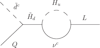
It is worth noticing here that one-loop contributions in the SSM will generate one of the usual lepton number violating terms mentioned in the introduction, , as shown in Fig. 12. The corresponding RGEs are:
| (155) |
However, this contribution is proportional to the neutrino Yukawa coupling, and therefore can be neglected in the computation.
Finally, for the VEVs we have
| (156) |
| (157) |
| (158) |
| (159) |
References
- [1] For reviews, see: H.P. Nilles, Phys. Rep. 110 (1984) 1; H.E. Haber and G.L. Kane, Phys. Rep. 117 (1985) 75; H.E. Haber, TASI lectures [arXiv:hep-ph/9306207]; S.P. Martin, in the book ‘Perspectives on supersymmetry’, World Scientific, p. 1 [arXiv:hep-ph/9709356].
- [2] For an update of the bounds on R-parity violating couplings, see: H.K. Dreiner, M. Kramer and B. O’Leary, Phys. Rev. D75 (2007) 114016 [arXiv:hep-ph/0612278], and references therein.
- [3] For a review, see: H.K. Dreiner, in the book ’Perspectives on supersymmetry’, World Scientific, p. 462 [arXiv:hep-ph/9707435].
- [4] J.A. Casas, E.K. Katehou and C. Muñoz, Oxford preprint, Nov. 1987, Ref: 1/88; Nucl. Phys. B317 (1989) 171; J.A. Casas and C. Muñoz, Phys. Lett. B212 (1988) 343 [arXiv:hep-ph/0309346].
- [5] For a recent review, see: C. Muñoz, Int. J. Mod. Phys. A19 (2004) 3093 [arXiv:hep-ph/0309346].
- [6] See e.g.: D.G. Cerdeño, C. Muñoz and O. Seto, arXiv:0807.3029 [hep-ph], and references therein.
- [7] For analyses of gravitino dark matter without R-parity, see: F. Takayama and M. Yamaguchi, Phys. Lett. B485 (2000) 388 [arXiv:hep-ph/0005214]; M. Hirsch, W. Porod and D. Restrepo, J. High Energy Phys. 03 (2005) 062 [arXiv:hep-ph/0503059]; W. Buchmuller, L. Covi, K. Hamaguchi, A. Ibarra and T. Yanagida, J. High Energy Phys. 03 (2007) 037 [arXiv:hep-ph/0702184]; G. Bertone, W. Buchmuller, L. Covi and A. Ibarra J. Cosm. Astrop. Phys. 11 (2007) 003 (arXiv:0709.2299 [astro-ph]); A. Ibarra and D. Tran Phys. Rev. Lett. 100 (2008) 061301 (arXiv:0709.4593 [astro-ph]), J. Cosm. Astrop. Phys. 07 (2008) 002 (arXiv:0804.4596 [astro-ph]).
- [8] For an analysis of axino dark matter without R-parity, see e.g.: H.B. Kim and J.E. Kim, Phys. Lett. 527 (2002) 18 [arXiv:hep-ph/0108101], and references therein.
- [9] For a recent review, see: R. Barbier et al., Phys. Rept. 420 (2005) 1 [arXiv:hep-ph/0406039].
- [10] See e.g.: B.C. Allanach, A. Dedes and H.K. Dreiner, Phys. Rev. D69 (2004) 115002, Erratum-ibid. D72 (2005) 079902 [arXiv:hep-ph/0309196]; D. Aristizabal Sierra, W. Porod, D. Restrepo and C.E. Yaguna, Phys. Rev. D78 (2008) 015015 (arXiv:0804.1907 [hep-ph]), and references therein.
- [11] L.J. Hall and M. Suzuki, Nucl. Phys. B231 (1984) 419; I.H. Lee, Phys. Lett. B138 (1984) 121; Nucl. Phys. B246 (1984) 120; S. Dawson, Nucl. Phys. B261 (1985) 297.
- [12] F. de Campos, M.A. Garcia-Jareño, A.S. Joshipura, J. Rosiek and J.W.F. Valle, Nucl. Phys. B451 (1995) 3 [arXiv:hep-ph/9502237]; R. Hempfling, arXiv:hep-ph/9609528; S. Davidson, M. Losada and N. Rius, Nucl. Phys. B587 (2000) 118 [arXiv:hep-ph/9911317]; M. Hirsch, M.A. Diaz, W. Porod, J.C. Romao and J.W.F. Valle, Phys. Rev. D62 (2000) 113008, Erratum-ibid. D65 (2002) 119901 [arXiv:hep-ph/0004115]; M. Hirsch and J.W.F. Valle, New J. Phys. 7 (2004) 76 [arXiv:hep-ph/0405015].
- [13] J.C. Romao, F. de Campos, M.A. Garcia-Jareño, M.B. Magro and J.W.F. Valle, Nucl. Phys. B482 (1996) 3 [arXiv:hep-ph/9604244]; M.C. Gonzalez-Garcia, J.C. Romao and J.W.F. Valle, Nucl. Phys. B391 (1993) 100; W. Porod, M. Hirsch, J.C. Romao and J.W.F. Valle, Phys. Rev. D63 (2001) 115004 [arXiv:hep-ph/0011248]; A. Bartl, M. Hirsch, T. Kernreiter, W. Porod and J.W.F. Valle, J. High Energy Phys. 11 (2003) 005 [arXiv:hep-ph/0306071]; M. Hirsch and W. Porod, Phys. Rev. D68 (2003) 115007 [arXiv:hep-ph/0307364].
- [14] C.S. Aulakh and R.N. Mohapatra, Phys. Lett. B119 (1982) 136; J. Ellis, G. Gelmini, C. Jarlskog, G.G. Ross and J.W.F. Valle, Phys. Lett. B150 (1985) 142; G.G. Ross and J.W.F. Valle, Phys. Lett. B151 (1985) 375.
- [15] P. Fayet, Nucl. Phys. B90 (1975) 104; H. P. Nilles, M. Srednicki and D. Wyler, Phys. Lett. B120 (1983) 346; J. M. Frere, D. R. T. Jones and S. Raby, Nucl. Phys. B222 (1983) 11; J. P. Derendinger and C. A. Savoy, Nucl. Phys. B237 (1984) 307.
- [16] J. R. Ellis, J. F. Gunion, H. E. Haber, L. Roszkowski and F. Zwirner, Phys. Rev. D39 (1989) 844; M. Drees, Int. J. Mod. Phys. A4 (1989) 3635; U. Ellwanger, M. Rausch de Traubenberg and C. A. Savoy, Phys. Lett. B315 (1993) 331 [arXiv:hep-ph/9307322]; P.N. Pandita, Phys. Lett. B318 (1993) 338, Z. Phys. C59 (1993) 575; S. F. King and P. L. White, Phys. Rev. D52 (1995) 4183 [arXiv:hep-ph/9505326]; U. Ellwanger and C. Hugonie, Eur. Phys. J. C13 (2000) 681 [arXiv:hep-ph/9812427].
- [17] D.G. Cerdeño, C. Hugonie, D. E. López-Fogliani, C. Muñoz and A. M. Teixeira, J. High Energy Phys. 12 (2004) 048 [arXiv:hep-ph/0408102]; G. Belanger, F. Boudjema, C. Hugonie, A. Pukhov, A. Semenov, J. Cosm. Astrop. Phys. 09 (2005) 001 [arXiv:hep-ph/0505142]; D.G. Cerdeño, E. Gabrielli, D. E. López-Fogliani, C. Muñoz and A. M. Teixeira, J. Cosm. Astrop. Phys. 06 (2007) 008 [arXiv:hep-ph/0701271]; C. Hugonie, G. Belanger and A. Pukhov J. Cosm. Astrop. Phys. 11 (2007) 001 (arXiv:0707.0628 [hep-ph]).
- [18] A. Djouadi et al. J. High Energy Phys. 07 (2008) 002 (arXiv:0801.4321 [hep-ph]); A. Djouadi, U. Ellwanger and A.M. Teixeira (arXiv:0803.0253 [hep-ph]); U. Ellwanger, C.-C. Jean-Louis and A.M. Teixeira, J. High Energy Phys. 05 (2008) 044 (arXiv:0803.2962 [hep-ph]).
- [19] P.N. Pandita and P. Francis Paulraj, Phys. Lett. B462 (1999) 294 [arXiv:hep-ph/9907561]; P.N. Pandita, Phys. Rev. D64 (2001) 056002 [arXiv:hep-ph/0103005]; M. Chemtob and P.N. Pandita, Phys. Rev. D73 (2006) 055012 [arXiv:hep-ph/0601159]; A. Abada and G. Moreau, J. High Energy Phys. 08 (2006) 044 [arXiv:hep-ph/0604216].
- [20] R. Kitano and K.Y. Oda, Phys. Rev. D61 (2000) 113001 [arXiv:hep-ph/9911327].
- [21] A. Abada, G. Bhattacharyya and G. Moreau, Phys. Lett. B642 (2006) 503 [arXiv:hep-ph/0606179].
- [22] C. Muñoz, in the book ’2006 Electroweak Interactions and Unified Theories’, XLIth Rencontres de Moriond, The Gioi Publishers (2006), p. 178 (arXiv:0705.2007 [hep-ph]).
- [23] Super-Kamiokande collaboration, Y. Fukuda et al., Phys. Rev. Lett. 81 (1998) 1562 [arXiv:hep-ex/9807003]; SNO collaboration, Q.R. Ahmad et al., Phys. Rev. Lett. 89 (2002) 011301 [arXiv:nucl-ex/0204008]; KamLAND collaboration, K. Eguchi et al., Phys. Rev. Lett. 90 (2003) 021802 [arXiv:hep-ex/0212021].
- [24] J.E. Kim and H.P. Nilles, Phys. Lett. B138 (1984) 150.
- [25] D. E. López-Fogliani and C. Muñoz, Phys. Rev. Lett. 97 (2006) 041801 [arXiv:hep-ph/0508297].
- [26] C. Muñoz, unpublished notes (1994).
- [27] Y. Farzan and J.W.F. Valle, Phys. Rev. Lett. 96 (2006) 011601 [arXiv:hep-ph/0509280].
- [28] B. Mukhopadhyaya and R. Srikanth, Phys. Rev. D74 (2006) 075001 [arXiv:hep-ph/0605109].
- [29] J. R. Ellis, K. Enqvist, D. V. Nanopoulos, K. A. Olive, M. Quiros and F. Zwirner, Phys. Lett. B176 (1986) 403; B. Ray and G. Senjanovic, Phys. Rev. D49 (1994) 2729 [hep-ph/9301240].
- [30] S. A. Abel, S. Sarkar and P. L. White, Nucl. Phys. B454 (1995) 663 [hep-ph/9506359].
- [31] S. A. Abel, Nucl. Phys. B480 (1996) 55 [hep-ph/9609323]; C. Panagiotakopoulos and K. Tamvakis, Phys. Lett. B446 (1999) 224 [hep-ph/9809475].
- [32]
G.F. Giudice and A. Masiero,
Phys. Lett. B206 (1988) 480.
- [33]
J.E. Kim and H.P. Nilles,
Phys. Lett. B263 (1991) 79;
E.J. Chun, J.E. Kim and H.P. Nilles,
Nucl. Phys. B370 (1992) 105;
- [34]
J.A. Casas and C. Muñoz,
Phys. Lett. B306 (1993) 288 [arXiv:hep-ph/9302227].
- [35] M. Masip and A. Rasin, Phys. Rev. D58 (1998) 035007 [arxiv:hep-ph/9803271].
- [36] J. Fidalgo, D.E. López-Fogliani, C. Muñoz and R. Ruiz de Austri, in preparation.
- [37] R. J. Zhang, Phys. Lett. B447 (1999) 89 [arXiv:hep-ph/9808299].
- [38] F. Gabbiani, E. Gabrielli,A. Masiero and L. Silvestrini, Nucl. Phys. B477 (1996) 321-352 [arXiv:hep-ph/9604387].
- [39] For a review, see: A. Brignole, L.E. Ibáñez and C. Muñoz, in the book ’Perspectives on supersymmetry’, World Scientific, p. 125 [arXiv:hep-ph/9707209].
- [40] Particle Data Group, C. Amsler et al., Phys. Lett. B667 (2008) 1.
- [41] The Tevatron electroweak working group for the CDF and D0 Collaboration, arXiv:0803.1683 [hep-ex].
- [42] S. G. Gorishnii, A. L. Kataev, S. A. Larin and L. R. Surguladze, Mod.Phys. Lett A4 (1990) 2703; L. V. Avdeev, O. V. Tarasov, A. A. Vladimirov, Phys. Lett. B96 (1980) 94; S. G. Gorishnii, A. L. Kataev and S. A. Larin, Phys. Lett. B135 (1984) 457.
- [43] W. A. Bardeen, A. J. Buras, D. W. Duke and T. Muta, Phys. Rev. D18 (1978) 3998.
- [44] J. A. Casas, J. R. Espinosa and H. E. Haber, Nucl. Phys. B526 (1998) 3 [arXiv:hep-ph/9801365].
- [45] I. G. Tsoulos and I. E. Lagaris, Comput. Phys. Commun. 174(2006) 152.
- [46] D. M. Pierce, J. A. Bagger, K. T. Matchev and R. j. Zhang, Nucl. Phys. B491 (1997) 3 [arXiv:hep-ph/9606211].
- [47] G. Passarino and M.J.G. Veltman, Nucl. Phys. B160 (1979) 151.
- [48] J.R. Espinosa and M. Quiros, Phys. Rev. Lett. 81 (1998) 516 [arXiv:hep-ph/9804235]; Y. Daikoku and D. Suematsu, Prog. Theor. Phys. 104 (2000) 827 [arXiv:hep-ph/0003206]; U. Ellwanger and C. Hugonie, Mod. Phys. Lett. A22 (2007) 1581 [arXiv:hep-ph/0612133].
- [49] See e.g.: D.G. Cerdeño, E. Gabrielli, S. Khalil, C. Muñoz and E. Torrente-Lujan, Nucl. Phys. B603 (2001) 231 [arXiv:hep-ph/0102270], and references therein.
- [50] R. Barbieri, L.J. Hall, Y. Nomura and V.S. Rychkov, Phys. Rev D75 (2007) 035007 [arXiv:hep-ph/0607332]; Y. Nomura and D. Poland, Phys. Rev D75 (2007) 015005 [arXiv:hep-ph/0608253].
- [51] J.R. Espinosa and M. Quiros, Phys. Lett. B279 (1992) 92; Phys. Lett. B302 (1993) 51 [arXiv: hep-ph/9212305].
- [52] M. Drees, Int. J. Mod. Phys. A4 (1989) 3635; J. R. Ellis, J. F. Gunion, H. E. Haber, L. Roszkowski and F. Zwirner, Phys. Rev. D39 (1989) 844; P. Binetruy and C. Savoy, Phys. Lett. B277 (1992) 453.
- [53] See e.g.: J.A. Casas, J.R. Espinosa and H.E. Haber, Nucl. Phys. B526 (1998) 3 [arXiv:hep/ph9801365], and references therein.