Work fluctuations in a nematic liquid crystal
Abstract
The orientation fluctuations of the director of a liquid crystal are measured, by a sensitive polarization interferometer, close to the Fréedericksz transition, which is a second order transition driven by an electric field. Using mean field theory, we define the work injected into the system by a change of the electric field and we calibrate it using Fluctuation-Dissipation Theorem. We show that the work fluctuations satisfy the Transient Fluctuation Theorem. An analytical justification of this result is given. The open problems for the out of equilibrium case are finally discussed.
pacs
05.40.-a,05.70.xz-a1 Introduction
The physics of small systems used in nanotechnology and biology has recently received an increased interest. In such systems, fluctuations of the work injected become of the order of the mean value, leading to unexpected and undesired effects. For example, the instantaneous energy transfer can flow from a cold source to a hot one. The probabilities of getting positive and negative injected work are quantitatively related in non equilibrium system using Fluctuation Theorem (FT) [1]-[5]. This theorem has been both theoretically and experimentally studied in Brownian systems described by a Langevin equation [6]-[14]. The Transient Fluctuation Theorem(TFT) of the injected work considers the work done on the system in the transient state, i.e. considering a time interval of duration which starts immediately after the external force has been applied to the system. For these systems, FT holds for all integration time and all fluctuation magnitudes :
| (1) |
where is the Boltzmann constant, the temperature of the heat bath and is the probability density function (PDF) of the injected work . is called symmetry function. In a recent paper [15], some surprising results have been obtained for the TFT in a spatially extended system where the fluctuations of the work injected by an electric field into a nematic liquid crystal (LC) have been studied. More precisely, the authors find an agreement between experimental results and TFT only for particular values of the observation time . We report in this article experimental results on the same system using a different measurement technic. We show that in our experiment, TFT holds for all integration time and all fluctuation magnitude. The paper is organized as follow. In the section 2, we describe the experimental setup. In the section 3, the work and the free energy of the LC system are defined. The experimental results are presented in section 4. Finally, we conclude in section 5.
2 Experimental setup
In our experimental apparatus, we measure the spatially averaged alignment of the LC molecules, whose local direction of alignment is defined by the unit vectors . The LC is confined between two parallel glass plates at a distance . The inner surfaces of the confining plates have transparent Indium-Tin-Oxyde (ITO) electrodes, used to apply an electric field . The plates surfaces are coated by a thin layer of polymer which is mechanically rubbed into one direction. This treatment of the glass plates align the molecules of the LC in a unique direction parallel to the surface (planar alignment), i.e. all the molecules near the surfaces have the same director parallel to -axis and (see figure 1a). This kind of coating excludes weak anchoring effect described in the literature [17]. The experiments are performed on nematic liquid crystal (5CB) produced by Merck in a cell of thickness m.
The LC is submitted to an electric field perpendicular to the plates by applying a voltage between the ITO electrodes. In order to avoid electrohydrodynamic effects of the motion of the ions invariably present in the liquid crystal, we apply an AC voltage at a frequency of kHz () [18, 19]. When the voltage exceeds a threshold value , the planar state becomes unstable and the LC molecules try to align parallel to the electric field (fig. 1a). This is known as the Fréedericksz transition which is second order. Above the critical value of the field, the equilibrium structure of the LC depends on the reduced control parameter defined as . The sample is thermostated at room temperature, i.e. K. The stability of the temperature is better than K over the duration of the experiment.

The measurement of the alignment of the LC molecules uses the anisotropic optical properties of the LC, i.e. the cell is a birefringent plate whose local optical axis is parallel to the director . This optical anisotropy can be precisely estimated by measuring the phase shift between two linearly polarized beams which cross the cell, one polarized along -axis (ordinary ray) and the other along the -axis (extraordinary ray). The experimental set-up employed is schematically shown in fig. 1c. The beam produced by a stabilized He-Ne laser ( nm) passes through the LC cell and it is finally back-reflected into the LC cell by a mirror. The lens between the mirror and the LC cell is used to compensate the divergency of the beam inside the interferometer. Inside the cell, the laser beam is parallel and has a diameter of about mm. The beam is at normal incidence to the cell and linearly polarized at from the -axis, i.e., can be decomposed in an extraordinary beam and in an ordinary one. The optical path difference, between the ordinary and extraordinary beams, is measured by a very sensitive polarization interferometer [21].
The phase shift takes into account the angular displacement in -plane, , and in -plane, (fig. 1b). For larger than the threshold value , depend only on and can be written as :
| (2) |
with (, ) the two anistotropic refractive indices [18, 19] and is the area of the measuring region of diameter in the (, ) plane. The global variable of our interest is defined as the spatially averaged alignment of the LC molecules, and more precisely :
| (3) |
Close to the critical value , using boundary conditions, the space dependance of along has the following form : , thus [18, 19, 20]. If remains small, takes a simple form in terms of :
| (4) |
After some algebra, we can show that the phase shift is a linear function of :
| (5) | |||
| (6) |
The phase , measured by the interferometer, is acquired with a resolution of bits at a sampling rate of Hz and then filtered at Hz in order to suppress the AC voltage at . The need of such a high acquisition frequency will be explained in the next section. The instrumental noise of the apparatus [21] is three orders of magnitude smaller than the amplitude of the fluctuations of induced by the thermal fluctuations of . In a recent paper, we have shown that is characterized by a mean value and fluctuations which have a lorentzian spectrum [22, 16].
We are interested here in the fluctuations of the work injected into the LC when it is driven away from an equilibrium state to another using a small change of the voltage (i.e. the control parameter), specifically:
| (7) |
We take care that the system is in equilibrium at by applying the value for a time much larger than the relaxation time () of the system. A typical measurement cycle is depicted in Fig. 2 where we plot (Fig. 2a) and (Fig. 2b) as functions of time. We repeat the same cycle 2500 times to compute, over this ensemble of experiments, the probability density function of the work injected during a time . We choose the amplitude of sufficiently small such that the mean response of the system to this excitation is comparable to the thermal noise amplitude, as can be seen in figure 2b) for and .

3 Landau equation and definition of the work
We define now the work injected into this system using the kind of forcing plotted in fig. 2a. The free energy is the sum of the electric energy and the potential energy :
| (8) |
Elastic free energy is a function of the director and its spatial derivative [18, 19] and electric free energy is where is the dielectric anisotropy of the LC ( is positive for 5CB). As the area of the measuring beam is much larger than the correlation length, we can neglect spatial derivative over and . Using the sinusoidal approximation for , i.e. [18], free energy has the following form :
| (9) | |||||
| (10) |
where is equal to , and , and are the three elastic constants of the LC. To simplify the analysis the dependance of in and can be neglected and the free energy takes the simple form:
| (11) |
where . From eq.11 we can obtain the equation of momentum [20]:
| (12) |
where is a viscosity coefficient and a thermal noise delta-correlated in time, such that :
| (13) |
where stands for ensemble average. First, we have to calibrate the system, i.e. determine the value of the constant that is a function of the area which is very difficult to precisely determine on the experiment. For this calibration, we use Fluctuation-Dissipation Theorem (FDT). We apply a small change of the voltage and, so of the control parameter, i.e. . We separate into the average part at and a deviation due to : , where is the stationary solution of eq.12 at . If the response is linear, the average value of is of the order of . In this limit, the equation of momentum can be rewritten :
| (14) |
The external torque, and so the conjugate variable to , is equal to
| (15) |
We define the integrated linear response function using an heaviside for :
| (16) |
where is the integrated response function of to . is related by FDT to the autocorrelation function,, of the fluctuations of , that is:
| (17) |
The global variable measured by the interferometer and defined in eq. 3 is . Thus the mean value of is and the fluctuations of can be related to the fluctuations of : . We measure the autocorrelation function of , . The response function of to is also related to : . Using fluctuation-dissipation theorem, we can measure the constant :
| (18) |
where .
We define now the work, , injected into the system when the control parameter is suddenly changed from to at (eq.7). Using equation 12, can be written as :
| (19) |
we consider that the external torque is . This expression can be integrated into :
| (20) |
Using the assumption of the limit of small and neglecting its dependance in the and directions, the work has a simple form in terms of :
| (21) |
Notice that if, is not too large, the quadratic term in this expression can be neglected, but it is not the case in general. The work is of course a fluctuating quantity because of the fluctuation of .
4 Fluctuations of the work injected into the system
4.1 Experimental results
The first step consists in calibrating the system. Indeed as we have already mentioned the parameter appearing in eq.18 depends on , i.e. the effective area of the laser beam inside the cell that is very difficult to estimate with a good accuracy. In order to calibrate the system we use FDT. In this case we use a sufficiently small perturbation to insure that the response is linear. Thus we obtain the integrated linear response of the system : . Then we measure the correlation . The function is a linear function of , as can be seen in figure 3 and the slope seems to be independent of . Using FDT, the slope is equal to ; by this method, we can calibrate the constant . We measure . Using in the equation for , the measured values of and , N (value for the LC 5CB) and m we estimate m2. This value is consistent with a mm which is very close to the estimated diameter of the laser beam inside the cell which is about mm. This justify our approach.

The system is at equilibrium at s and we are now interested in the work done by the change of during a time , . We need a high acquisition frequency to reduce experimental errors in the determination of the first point of each cycle . The probability density function of are plotted in figure 4 for different values of . We find that the PDFs are Gaussian for all values of and the average value of is equal to a few . We also notice that the probability of having negative values decreases when is increased. The symmetry function is plotted in fig. 4b. It is a linear function of for any , that is . Within experimental errors, we measure the slope . Thus, for our experimental system, the TFT is verified for any time .

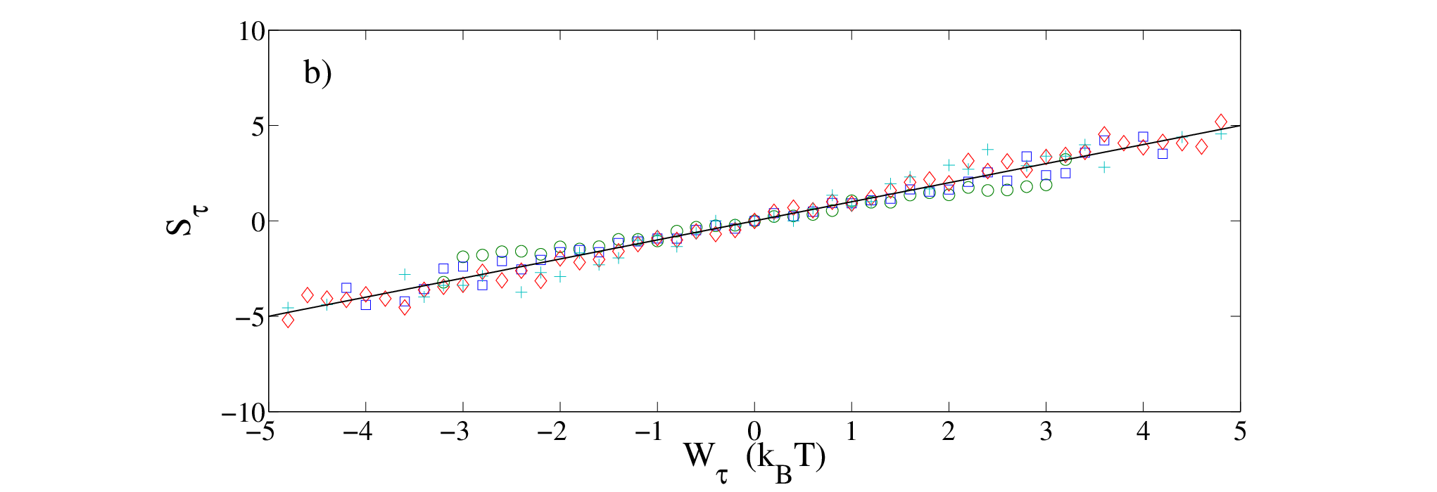
To test the importance of the quartic terms in the expression of the work, we have done the same experiments using a higher value of the control parameter . The perturbation remains small (see figure 5). The quadratic terms in the expression of the work cannot be neglected in this situation. We find that the PDFs of the work are also Gaussian for all the integration times. This is normal because the perturbation is such small that we are in the realm of the applicability of the FDT. The symmetry function is plotted in fig. 5b. It is a linear function of for any . Within experimental errors, we measure the slope equal to . Thus, for our experimental system, the TFT is verified for any time .


4.2 Comparison with theory
These results can be justified for small and . Decomposing into the sum of a mean part and a fluctuating one , i.e. . The distributions of the injected work are Gaussian for all values of , so the symmetry function takes a simple form :
| (22) |
where is the variance of the fluctuation of the injected work. The mean value of the work is for small and small :
| (23) | |||||
| (24) |
The variance of the fluctuations is given by :
| (25) | |||||
| (26) |
Using FDT, we obtain that , thus FT is satisfied for all integration times and all fluctuation magnitudes as can be seen in fig. 4b).
5 Conclusion
In conclusion, we have defined in a LC cell close to Fréedericksz transition the work injected into the system by the change of during a time using the assumption of small angle and neglecting its dependance in and directions. We have shown that the TFT holds for the work injected in a spatially extended system for all integration times and all fluctuation magnitudes. We have tested this result for another thickness of the LC cell and other values of . It is interesting to notice that this experimental test is the first for a spatially extended system in the presence of a non linear potential. This is in contrast to the result of ref [15]. The reason of this discrepancy is that they neglect in the definition of the work (eq.21) the square term in . This cannot be done when a large is used as in the case of ref.[15].
Our results are a preliminary study for future investigation on unsolved problems such as the applicability of Transient Fluctuation Theorem in an out-of-equilibrium system such as an aging system or a rapid quench.
References
References
- [1] G. Gallavotti, E.G.D. Cohen, Phys. Rev. Lett. 1995 74 2694; G. Gallavotti, E.G.D. Cohen, J. Stat. Phys. 1995 80(5-6) 931
- [2] D.J. Evans, D.J. Searles Phys. Rev. E 1994 50 1645; D.J. Evans, D.J. Searles, Advances in Physics 2002 51(7) 1529; D.J. Evans, D.J. Searles, L. Rondoni Phys. Rev. E 2005 71(5) 056120
- [3] J. Kurchan, J. Phys. A : Math. Gen. 1998 31 3719
- [4] J.L. Lebowitz and H. Spohn, J. Stat. Phys., 1999 95 333
- [5] R.J. Harris, G.M. Schütz, J. Stat. Mech. : Theory and Experiment, 2007 P07020
- [6] V. Blickle, T. Speck, L. Helden, U. Seifert, C. Bechinger, Phys. Rev. Lett., 2006 96 070603
- [7] S. Joubaud, N.B. Garnier, S. Ciliberto, J. Stat. Mech.: Theory and Experiment, 2007 P09018
- [8] J. Farago, J. Stat. Phys., 2002, 107 781; Physica A 2004 331 69
- [9] R. van Zon, E.G.D. Cohen, Phys. Rev. Lett. 2003 91(11) 110601; R. van Zon, E.G.D. Cohen, Phys. Rev. E 2003 67 046102; R. van Zon, S. Ciliberto, E.G.D. Cohen, Phys. Rev. Lett. 2004 92(13)130601
- [10] G.M. Wang, E.M. Sevick, E. Mittag, D.J. Searles, D.J. Evans, Phys. Rev. Lett., 2002 89 050601; G.M. Wang, J.C. Reid, D.M. Carberry, D.R.M. Williams, E.M. Sevick, D.J. Evans, Phys. Rev. E 2005 71 046142
- [11] N. Garnier and S. Ciliberto, Phys. Rev. E, 2005 71 060101(R)
- [12] A. Imparato, L. Peliti, G. Pesce, G. Rusciano, A. Sasso, Phys. Rev. E 2007 76 050101(R); A. Imparato, L. Peliti, Europhys. Lett., 2005 70 740-746
- [13] F. Douarche, S. Joubaud, N. Garnier, A. Petrosyan and S. Ciliberto, Phys. Rev. Lett. 2006 97 140603
- [14] T. Taniguchi and E.G.D. Cohen, J. Stat. Phys. 2007 127 1-41; T. Taniguchi and E.G.D. Cohen, J Stat Phys 2008 130 633-667
- [15] S. Datta, A. Roy, 2008 cond-mat arXiv:0805:0952
- [16] S. Joubaud, A. Petrosyan, S.Ciliberto, N. Garnier, 2008 Phys. Rev. Lett. 100 180601
- [17] J. Cognard, 1982 Molecular crystals and liquid crystals supplement series 1 1
- [18] P.G. De Gennes and J. Prost, 1974, Clarendon Press, Oxford, ch 5
- [19] P. Oswald and P. Pieranski, 2005, Taylor & Francis, ch 4, ch 5
- [20] M. San Miguel, 1985 Phys. Rev. A 32(6) 3811
- [21] L. Bellon, S. Ciliberto, H. Boubaker, L. Guyon, 2002 Optics Communications 207 49-56
- [22] P. Galatola and M. Rajteri, 1994 Phys. Rev. 49 623.