On Resource Allocation in Fading Multiple Access Channels - An Efficient Approximate Projection Approach
Abstract
We consider the problem of rate and power allocation in a multiple-access channel. Our objective is to obtain rate and power allocation policies that maximize a general concave utility function of average transmission rates on the information theoretic capacity region of the multiple-access channel. Our policies does not require queue-length information. We consider several different scenarios. First, we address the utility maximization problem in a non-fading channel to obtain the optimal operating rates, and present an iterative gradient projection algorithm that uses approximate projection. By exploiting the polymatroid structure of the capacity region, we show that the approximate projection can be implemented in time polynomial in the number of users. Second, we consider resource allocation in a fading channel. Optimal rate and power allocation policies are presented for the case that power control is possible and channel statistics are available. For the case that transmission power is fixed and channel statistics are unknown, we propose a greedy rate allocation policy and provide bounds on the performance difference of this policy and the optimal policy in terms of channel variations and structure of the utility function. We present numerical results that demonstrate superior convergence rate performance for the greedy policy compared to queue-length based policies. In order to reduce the computational complexity of the greedy policy, we present approximate rate allocation policies which track the greedy policy within a certain neighborhood that is characterized in terms of the speed of fading.
Index Terms:
Multiple access, resource allocation, power control, utility maximization, fading channel, rate splitting.I Introduction
Dynamic allocation of communication resources such as bandwidth or transmission power is a central issue in multiple access channels in view of the time varying nature of the channel and the interference effects. Most of the existing literature focuses on specific communication schemes such as TDMA (time-division multiple access) [1], CDMA (code-division multiple access) [2, 3], and OFDM (Orthogonal Frequency Division Multiplexing) [4] systems. An exception is the work by Tse et al. [5], which consider the notion of throughput capacity for the fading channel with Channel State Information (CSI). The throughput capacity is the notion of Shannon capacity applied to the fading channel, where the codeword length can be arbitrarily long to average over the fading of the channel. Tse et al. [5] consider allocation of rate and power to maximize a linear utility function of the transmission rates over the throughput region, which characterizes the points on the boundary of the throughput capacity region.
In this paper, we consider the problem of rate and power allocation in a multiple access channel with perfect CSI. Contrary to the linear case in [5], we consider maximizing a general utility function of transmission rates over the throughput capacity region. Such a general concave utility function allows us to capture different performance metrics such as fairness or delay (cf. Shenker [6], Srikant [7]). Our contributions can be summarized as follows.
We first consider a non-fading multiple-access channel where we introduce a gradient projection algorithm for the problem of maximizing a concave utility function of transmission rates over the capacity region. We establish the convergence of the method to the optimal rate allocation. Since the capacity region of the multiple-access channel is described by a number of constraints exponential in the number of users, the projection operation used in the method can be computationally expensive. To reduce the computational complexity, we introduce a new method that utilizes approximate projections. By exploiting the polymatroid structure of the capacity region, we show that the approximate projection operation can be implemented in time polynomial in number of users by using submodular function minimization algorithms. Moreover, we present a more efficient algorithm for the approximate projection problem which relies on rate-splitting [8]. This algorithm also provides the extra information that allows the receiver to decode the message by successive cancelation.
Second, we consider a fading multiple access channel and study the case where channel statistics are known and transmission power can be controlled at the transmitters. Owing to strict convexity properties of the capacity region along the boundary, we show that the resource allocation problem for a general concave utility is equivalent to another problem with a linear utility. Hence, the optimal resource allocation policies are obtained by applying the results in [5] for the linear utility. Given a general utility function, the conditional gradient method is used to obtain the corresponding linear utility.
If the transmitters do not have the power control feature and channel statistics are not known, the throughput capacity region is a polyhedron and the strictly convexity properties of the region do not hold any more. Hence, the previous approach is not applicable. In this case, we consider a greedy policy, which maximizes the utility function for any given channel state. This policy is suboptimal, however, we can bound the performance difference between the optimal and the greedy policies. We show that this bound is tight in the sense that it goes to zero either as the utility function tends to a linear function of the rates or as the channel variations vanish.
The greedy policy requires exact solution of a nonlinear program in each time slot, which makes it computationally intractable. To alleviate this problem, we present approximate rate allocation policies based on the gradient projection method with approximate projection and study its tracking capabilities when the channel conditions vary over time. In our algorithm, the solution is updated in every time slot in a direction to increase the utility function at that time slot. But, since the channel may vary between time-slots, the level of these temporal channel variations become critical to the performance. We explicitly quantify the impact of the speed of fading on the performance of the policy, both for the worst-case and the average speed of fading. Our results also capture the effect of the degree of concavity of the utility functions on the average performance.
An important literature relevant to our work appears in the context of cross-layer design, where joint scheduling-routing-flow control algorithms have been proposed and shown to achieve utility maximization for concave utility functions while guaranteeing network stability (e.g. [9, 10, 11, 12]). The common idea behind these schemes is to use properly maintained queues to make dynamic decisions about new packet generation as well as rate allocation.
Some of these works ([10, 11]) explicitly address the fading channel conditions, and show that the associated policies can achieve rates arbitrarily close to the optimal based on a design parameter choice. However, the rate allocation with these schemes requires that a large optimization problem requiring global queue-length information be solved over a complex feasible set in every time slot. Clearly, this may not always be possible owing to the limitations of the available information, the processing power, or the complexity intrinsic to the feasible set. Requirement for queue-length information may impose much more overhead on the system than channel state information. On the other hand, even in the absence of fading, the interference constraints among nearby nodes’ transmissions may make the feasible set so complex that the optimal rate allocation problem becomes NP-hard (see [13]). Moreover, the convergence results of queue-length based policies ([10, 11]) are asymptotic, and our simulation results show that such policies may suffer from poor convergence rate. In fact, duration of a communication session may not be sufficient for these algorithms to approach the optimal solution while suboptimal policies such as the greedy policy seems to have superior performance when communication time is limited, even though the greedy policy does not use queue-length information.
In the absence of fading, several works have proposed and analyzed approximate randomized and/or distributed rate allocation algorithms for various interference models to reduce the computational of the centralized optimization problem of the rate allocation policy ([14, 9, 15, 13, 16, 17]). The effect of these algorithms on the utility achieved is investigated in [13, 18]. However, no similar work exists for fading channel conditions, where the changes in the fading conditions coupled with the inability to solve the optimization problem instantaneously make the solution much more challenging.
Other than the papers cited above, our work is also related to the work of Vishwanath et al. [19] which builds on [5] and takes a similar approach to the resource allocation problem for linear utility functions. Other works address different criteria for resource allocation including minimizing delay by a queue-length based approach [20], minimizing the weighted sum of transmission powers [21], and considering Quality of Service (QoS) constraints [22]. In contrast to this literature, we consider the utility maximization framework for general concave utility functions.
The remainder of this paper is organized as follows: In Section II, we introduce the model and describe the capacity region of a fading multiple-access channel. In Section III, we consider the utility maximization problem in a non-fading channel and present the gradient projection method with approximate projection. In Section IV, we address the resource allocation problem with power control and known channel statistics. In Section V, we consider the same problem without power control and knowledge of channel statistics. We present the greedy policy and approximate rate allocation policies and study their tracking behavior. Section VI provides the simulation results, and we give our concluding remarks in Section VII.
Regarding the notation, we denote by the -th component of a vector . We denote the nonnegative orthant by , i.e., . We write to denote the transpose of a vector . We use the notation for the probability of an event in the Borel -algebra on . The exact projection operation on a closed convex set is denoted by , i.e., for any closed convex set and , we have , where denotes the Euclidean norm.
II System Model
We consider transmitters sharing the same media to communicate to a single receiver. We model the channel as a Gaussian multiple access channel with flat fading effects,
| (1) |
where and are the transmitted waveform and the fading process of the -th transmitter, respectively, and is properly bandlimited Gaussian noise with variance . We assume that the fading processes of all transmitters are jointly stationary and ergodic, and the stationary distribution of the fading process has continuous density. We assume that all the transmitters and the receiver have instant access to channel state information. In practice, the receiver measures the channels and feeds back the channel information to the transmitters. The implicit assumption in this model is that the channel variations are much slower than the data rate, so that the channel can be measured accurately at the receiver and the amount of feedback bits is negligible compared to that of transmitting information.
Definition 1
The temporal variation in fading is modeled as follows:
| (2) |
where the s are nonnegative random variables independent across time slots for each . We assume that for each , the random variables are uniformly bounded from above by , which we refer to as the maximum speed of fading. Under slow fading conditions, the distribution of is expected to be more concentrated around zero.
Consider the non-fading case where the channel state vector is fixed. The capacity region of the Gaussian multiple-access channel with no power control is described as follows [23],
| (3) |
where and are the -th transmitter’s power and rate, respectively. denotes Shannon’s formula for the capacity of the AWGN channel given by
| (4) |
For a multiple-access channel with fading, but fixed transmission powers , the throughput capacity region is given by averaging the instantaneous capacity regions with respect to the fading process [24],
| (5) |
where is a random vector with the stationary distribution of the fading process.
A power control policy is a function that maps any given fading state to the powers allocated to the transmitters . Similarly, we can define the rate allocation policy, , as a function that maps the fading state to the transmission rates, . For any given power-control policy , the capacity region follows from (5) as
| (6) |
Tse et al. [5] have shown that the throughput capacity of a multiple access fading channel is given by
| (7) |
where is the set of all power control policies satisfying the average power constraint. Let us define the notion of boundary or dominant face for any of the capacity regions defined above.
Definition 2
The dominant face or boundary of a capacity region, denoted by , is defined as the set of all -tuples in the capacity region such that no component can be increased without decreasing others while remaining in the capacity region.
III Rate Allocation in a Non-fading Channel
In this section, we address the problem of finding the optimal operation rates in a non-fading multiple-access channel. Without loss of generality, we fix the channel state vector to unity throughout this section, and denote the capacity region by a simpler notation instead of , where denotes the transmission power. Consider the following utility maximization problem for a -user channel.
| maximize | |||||
| subject to | (8) |
where and are -th user rate and power, respectively. The utility function is assumed to satisfy the following conditions.
Assumption 1
The following conditions hold:
- (a)
The utility function is concave with respect to vector .
- (b)
is monotonically increasing with respect to , for .
Assumption 2
There exists a scalar such that
where denotes the subdifferential of at , i.e., the set of all subgradients 11 1 The vector is a subgradient of a concave function at , if and only if for all . of at .
Note that Assumption 2 is standard in the analysis of subgradient methods for non-differentiable optimization problems [25]. The maximization problem in (8) is a convex program and the optimal solution can be obtained by several optimization methods such as the gradient projection method. The gradient projection method with exact projection is typically used for problems where the projection operation is simple, i.e., for problems with simple constraint sets such as the non-negative orthant or a simplex. However, the constraint set in (8) is defined by exponentially many constraints, making the projection problem computationally intractable. To alleviate this problem, we use an approximate projection, which is obtained by successively projecting on violated constraints.
Definition 3
Let , where has non-negative entries. Let violate the constraint , for . The approximate projection of on , denoted by , is given by
where denotes the exact projection on the hyperplane .
An example of approximate projection on a two-user multiple-access capacity region is illustrated in Figure 1. As shown in the figure, the result of approximate projection is not necessarily unique. In the following, when we write , it refers to an approximate projection for an arbitrary order of projections on the violated hyperplanes. Although the approximate projection is not unique, it is pseudo-nonexpansive as claimed in the following Lemma.

Lemma 1
The approximate projection given by Definition 3 has the following properties:
- (i)
For any , is feasible with respect to set , i.e., .
- (ii)
is pseudo-nonexpansive, i.e.,
(9)
Proof:
For part (i), it is straightforward to see that is given by (cf. [26] Sec. 2.1.1) P_i(y) = y - a i ’y - b i ∥a i ∥ a_i. Since has only non-negative entries, all components of are decreased after projection and hence, the constraint will not be violated in the subsequent projections. This shows that given an infeasible vector , the approximate projection operation given in Definition 3 yields a feasible vector with respect to set .
Part (ii) can be verified by using the nonexpansiveness property of projection on a closed convex set (See Proposition 2.1.3 of [26]) for times. Since is a fixed point of for all , we have
| (10) | |||||
Q.E.D.
Here, we present the gradient projection method with approximate projection to solve the problem in (8). The -th iteration of the gradient projection method with approximate projection is given by
| (11) |
where is a subgradient of at , and denotes the stepsize. Figure 2 demonstrates gradient projection iterations for a two-user multiple access channel. The following theorem provides a sufficient condition which can be used to establish convergence of (11) to the optimal solution.

Theorem 1
Proof:
We have
By concavity of , we have
| (14) |
Hence,
If the stepsize satisfies (12), the above relation yields the following ∥R^k + α^k g^k - R^*∥ ¡ ∥R^k - R^*∥.
Now by applying pseudo-nonexpansiveness of the approximate projection we have
Q.E.D.
Theorem 2
Proof:
See Proposition 8.2.7 of [25]. Q.E.D.
The convergence analysis for this method can be extended for different stepsize selection rules. For instance, we can employ diminishing stepsize, i.e.,
or more complicated dynamic stepsize selection rules such as the path-based incremental target level algorithm proposed by Brännlund [27] which guarantees convergence to the optimal solution [25], and has better convergence rate compared to the diminishing stepsize rule.
III-A Complexity of the Projection Problem
Even though the approximate projection is simply obtained by successive projection on the violated constraints, it requires to find the violated constraints among exponentially many constraints describing the constraint set. In this part, we exploit the special structure of the capacity region so that each gradient projection step in (11) can be performed in polynomial time in .
Definition 4
Let be a function defined over all subsets of . The function is submodular if
| (15) |
Lemma 2
Define as follows:
| (16) |
If for all , then is submodular. Moreover, the inequality holds with equality if and only if , or .
Proof:
The proof is simply by plugging the definition of in inequality (15). In particular,
| (17) | |||||
Since , the above inequality holds with equality if and only if , or . This condition is equivalent to either or contains the other. Q.E.D.
Theorem 3
For any , finding the most violated capacity constraint in (3) can be written as a submodular function minimization (SFM) problem, that is unconstrained minimization of a submodular function over all .
Proof:
We can rewrite the capacity constraints of as
| (18) |
Thus, the most violated constraint at corresponds to
By Lemma 2 is a submodular function. Since summation of a submodular and a linear function is also submodular, the problem above is of the form of submodular function minimization. Q.E.D.
It was first shown by Grötschel et al. [28] that an SFM problem can be solved in polynomial time. The are several fully combinatorial strongly polynomial algorithms in the literature. The best known algorithm for SFM proposed by Orlin [29] has running time . Note that approximate projection does not require any specific order for successive projections. Hence, finding the most violated constraint is not necessary for approximate projection. In view of this fact, a more efficient algorithm based on rate-splitting is presented in Appendix A, to find a violated constraint. It is shown in Theorem 11 that the rate-splitting-based algorithm runs in time, where is the number of users.
Although a violated constraint can be obtained in polynomial time, it does not guarantee that the approximate projection can be performed in polynomial time. Because it is possible to have exponentially many constraints violated at some point and hence the total running time of the projection would be exponential in . However, we show that for a small enough stepsize in the gradient projection iteration (11), no more than constraints can be violated at each iteration. Let us first define the notions of expansion and distance for a polyhedra.
Definition 5
Let be a polyhedron described by a set of linear inequalities, i.e.,
| (19) |
Define the expansion of by , denoted by , as the polyhedron obtained by relaxing all the constraints in (19), i.e., where is the vector of all ones.
Definition 6
Let and be two polyhedra described by a set of linear constraints. Let be an expansion of by as defined in Definition 5. The distance between and is defined as the minimum scalar such that and .
Lemma 3
Proof:
Existence of a positive scalar satisfying (20) follows directly from Lemma 2, using the fact that neither nor contains the other one.
Suppose for some , there are violated constraints of . Since it is not possible to have non-empty nested sets in , there are at least two violated constraints corresponding to some sets where , and
| (21) | |||||
| (22) |
Since is feasible in the relaxed region,
| (23) | |||||
| (24) |
Note that if , (23) reduces to , which is a valid inequality.
By summing the above inequalities we conclude
| (25) |
which is a contradiction. Q.E.D.
Theorem 4
If the stepsize in the -th iteration (11) satisfies
| (26) |
then at most constraints of the capacity region can be violated at each iteration step.
Proof:
We first show that inequality in (20) holds for the following choice of :
| (27) |
In order to verify this, rewrite the right hand side of (20) as
The inequalities can be justified by using the monotonicity of the logarithm function and the fact that is non-empty because .
Now, let be feasible in the capacity region, . For every , we have
| (28) | |||||
where the first inequality follows from Assumption 1(b), Assumption 2, and Eq. (26). The second inequality holds because for any unit vector , it is true that
| (29) |
Thus, if satisfies (26) then , for some for which (20) holds. Therefore, by Lemma 3 the number of violated constraints does not exceed . Q.E.D.
In view of the fact that a violated constraint can be identified in time (see the Algorithm in Appendix A), Theorem 4 implies that, for small enough stepsize, the approximate projection can be implemented in time.
In section V, we will develop algorithms that use the gradient projection method for dynamic rate allocation in a time varying channel.
IV Dynamic Rate and Power Allocation in Fading Channel with Known Channel Statistics
In this section, we assume that the channel statistics are known. Our goal is to find feasible rate and power allocation policies denoted by and , respectively, such that , and . Moreover,
| (30) |
where is a given utility function and is assumed to be differentiable and satisfy Assumption 1.
For the case of a linear utility function, i.e., for some , Tse et al. [5] have shown that the optimal rate and power allocation policies are given by the optimal solution to a linear program, i.e.,
| (31) |
where is the channel state realization, and is a Lagrange multiplier satisfying the average power constraint, i.e., is the unique solution of the following equations
| (32) |
where and are, respectively, the cumulative distribution function (CDF) and the probability density function (PDF) of the stationary distribution of the channel state process for transmitter .
Exploiting the polymatroid structure of the capacity region, problem (31) can be solved by a simple greedy algorithm (see Lemma 3.2 of [5]). It is also shown in [5] that, for positive , the optimal solution, , to the problem in (30) is uniquely obtained. Given the distribution of channel state process, denoted by and , we have
| (33) |
The uniqueness of follows from the fact that the stationary distribution of the channel state process has a continuous density [5]. It is worth mentioning that (33) parametrically describes the boundary of the capacity region which is precisely defined in Definition 2. Thus, there is a one-to-one correspondence between the boundary of and the positive vectors with unit norm.
Now consider a general concave utility function satisfying Assumption 1. It is straightforward to show that , the optimal solution to (30), is unique. Moreover, by Assumption 1(b) it lies on the boundary of the throughput region. Now suppose that is given by some genie. We can choose and , as a replacement for the nonlinear utility. By checking the optimality conditions, it can be seen that is also the optimal solution of the problem in (30), i.e.,
| (34) |
Thus, we can employ the greedy rate and power allocation policies in (31) for the linear utility function , and achieve the optimal average rate for the nonlinear utility function . Therefore, the problem of optimal resource allocation reduces to computing the vector . Note that the throughput capacity region is not characterized by a finite set of constraints, so standard optimization methods such as gradient projection or interior-point methods are not applicable in this case. However, the closed-form solution to maximization of a linear function on the throughput region is given by (33). This naturally leads us to the conditional gradient method [26] to compute . The -th iteration of the method is given by
| (35) |
where is the stepsize and is obtained as
| (36) |
where denotes the gradient vector of at . Since the utility function is monotonically increasing by Assumption 1(b), the gradient vector is always positive and, hence, the unique optimal solution to the above sub-problem is obtained by (33), in which is replaced by . By concavity of the utility function and convexity of the capacity region, the iteration (35) will converge to the optimal solution of (30) for appropriate stepsize selection rules such as the Armijo rule or limited maximization rule (cf. [26] pp. 220-222).
Note that our goal is to determine rate and power allocation policies. Finding allows us to determine such policies by the greedy policy in (31) for . It is worth mentioning that all the computations for obtaining are performed once in the setup of the communication session. Here, the convergence rate of the conditional gradient method is generally not of critical importance.
V Dynamic Rate Allocation without Knowledge of Channel Statistics
In this part we assume that the channel statistics are not known and that the transmission powers are fixed to . In practice, this scenario occurs when the transmission power may be limited owing to environmental limitations such as human presence, or limitations of the hardware.
The capacity region of the fading multiple access channel for this scenario is a polyhedron given by (5). Similarly to the previous case, the goal is to find an optimal rate allocation policy with respect to a given utility function, which we formally define next.
Definition 7
[Optimal Policy] The optimal rate allocation policy denoted by is a mapping that satisfies for all , such that
| argmax | (37) | ||||
| subject to |
It is worth noting that the approach used to find the optimal resource allocation policies for the case with known channel statistics does not apply to this scenario, because is a polyhedron and hence, unlike in Section IV the uniqueness of the optimal solution, for any positive vector does not hold anymore.
Here we present a greedy rate allocation policy and compare its performance with the unknown optimal policy. The performance of a particular rate allocation policy is defined as the utility function evaluated at the average rate achieved by that policy.
Definition 8
[Greedy Policy] A greedy rate allocation policy, denoted by , is given by
| argmax | (38) | ||||
| subject to |
i.e., for each channel state, the greedy policy chooses the rate vector that maximizes the utility function over the corresponding capacity region.
The utility function is assumed to satisfy the following conditions.
Assumption 3
For every , let . The following conditions hold:
- (a)
There exists a scalar such that for all ,
where
(39) - (b)
There exists a scalar such that for all ,
Assumption 3(a) is a weakened version of Assumption 2, which imposes a bound on subgradients of the utility function. This assumption only requires bound on the subgradient in a neighborhood of the optimal solution and away from the origin, which is satisfied by a larger class of functions. Assumption 3(b) is a strong concavity type assumption. In fact, strong concavity of the utility implies Assumption 3(b), but it is not necessary. The scalar becomes small as the utility tends to have a linear structure with level sets tangent to the dominant face of the capacity region. Assumption 3 holds for a large class of utility functions including the well known -fair functions given by
| (40) |
which do not satisfy Assumption 2.
Note that the greedy policy is not necessarily optimal for general concave utility functions. Consider the following relations
| (41) | |||||
where the first and third inequality follow from the feasibility of the optimal and the greedy policy for any channel state, and the second inequality follows from Jensen’s inequality by concavity of the utility function.
In the case of a linear utility function we have , so equality holds throughout in (41) and is indeed the optimal rate allocation policy. For nonlinear utility functions, the greedy policy can be strictly suboptimal.
However, the greedy policy is not arbitrarily worse than the optimal one. In view of (41), we can bound the performance difference, , by bounding or from above. We show that the first bound goes to zero as the channel variations become small and the second bound vanishes as the utility function tends to have a more linear structure.
Before stating the main theorems, let us introduce some useful lemmas. The first lemma asserts that the optimal and greedy policies assign rates on the dominant face of the capacity region.
Lemma 4
Proof:
Part (a) is direct consequence of Assumption 1(b) and Definition 2. If the optimal solution to the utility maximization problem is not on the dominant face, there exists a user such that we can increase its rate and keep all other user’s rates fixed while staying in the capacity region. Thus, we are able to increase the utility by Assumption 1(b), which leads to a contradiction.
For part (b), first note that with the same argument as above we have
| (42) |
Thus, , with probability one, because , for all . Therefore, by definition of MAC capacity region in (3) we conclude , with probability one. Q.E.D.
The following lemma extends Chebyshev’s inequality for capacity regions. It states that, with high probability, the time varying capacity region does not deviate much from its mean.
Lemma 5
Let be a random vector with the stationary distribution of the channel state process, mean and covariance matrix . Then
| (44) |
where is defined as
| (45) |
where
| (46) |
Proof:
See Appendix B. Q.E.D.
The system parameter in Lemma 5 is proportional to channel variations, and we expect it to vanish for very small channel variations. The following lemma ensures that the distance between the optimal solutions of the utility maximization problem over two regions is small, provided that the regions are close to each other.
Lemma 6
Proof:
See Appendix C. Q.E.D.
The following theorem combines the results of the above two lemmas to obtain a bound on the performance difference of the greedy and the optimal policy.
Theorem 5
Proof:
Pick any . Define the event, as V = { H: d_H(C_g(P, H), C_a(P)) ≤δ}.
By Lemma 5, the probability of this event is at least . Using Jensen’s inequality as in (41) we can bound the left-hand side of (48) as follows
| (49) | |||||
In the above relations, the first inequality follows from the fact that , and the second inequality holds because of the non-negativity of .
On the other hand, by incorporating Lemma 4 in Assumption 3(a) we have —u(R^*) -u( ¯ R (H)) — ≤B(δ) ∥ ¯ R (H) - R^*∥.
Now by Assumption 3 we can employ Lemma 6 to conclude the following from the above relation:
which implies
| (50) |
Q.E.D.
Theorem 5 provides a bound parameterized by . For very small channel variations, becomes small. Therefore, the parameter can be picked small enough such that the bound in (48) tends to zero. Figure 3 illustrates the behavior of right hand side of Eq. (48) as a function of for different values of . For each value of , the upper bound is minimized for a specific choice of , which is illustrated by a dot in Figure 3. As demonstrated in the figure, for smaller channel variations, a smaller gap is achieved and the parameter that minimizes the bound decreases.
The next theorem provides another bound demonstrating the impact of the structure of the utility function on the performance of the greedy policy.

Theorem 6
Proof:
Similarly to the proof of Theorem 5, for any define the event as
| (54) |
By Lemma 5, this event has probability at least . Lemma 4 asserts that the optimal policy almost surely allocate rate vectors on the dominant face of . Therefore, for almost all , the optimal policy satisfies the following
| (55) |
Thus, for almost all , we have —R_i^*(H) - R_i^*— ≤ σ H ϵ + E_H[ 1 2 log( (1+H i P i )(1+∑ j ≠i H j P j ) 1+∑ j=1 M H j P j )].
Therefore,
| (56) | |||||
Now let us write the Taylor expansion of at in the direction of ,
| (57) | |||||
In the above relation, let for all . The utility function is concave, so its Hessian is negative definite and we can combine (56) with the above relation to write
| (58) |
Taking the expectation conditioned on , and using the fact that we have the following
| (59) |
Hence, we conclude
where the first inequality is verified by (41), and the third inequality follows from non-negativity of the utility function and the inequality in (59). Q.E.D.
Similarly to Theorem 5, Theorem 6 provides a bound parameterized by . As the utility function tends to have a more linear structure, tends to zero. For instance, is proportional to for a weighted sum -fair utility function. Hence, we can choose small such that the right hand side of (51) goes to zero. The behavior of this upper bound for different values of is similar to the one plotted in Figure 3.
In summary, the performance difference between the greedy and the optimal policy is bounded from above by the minimum of the bounds provided by Theorem 5 and Theorem 6.
Even though the greedy policy can perform closely to the optimal policy, it requires solving a nonlinear program in each time slot. For each channel state, finding even a near-optimal solution of the problem in (38) requires a large number of iterations, making the online evaluation of the greedy policy impractical. In the following section, we introduce an alternative rate allocation policy, which implements a single gradient projection iteration of the form (11) per time slot.
V-A Approximate Rate Allocation Policy
In this part, we assume that the channel state information is available at each time slot , and the computational resources are limited such that a single iteration of the gradient projection method in (11) can be implemented in each time slot. In order to simplify the notation in this part and avoid unnecessary technical details, we consider a stronger version of Assumption 3(b).
Assumption 4
Let . Then there exists a positive scalar such that
Definition 9
[Approximate Policy] Given some fixed integer , we define the approximate rate allocation policy, , as follows:
| (60) |
where
| (61) |
and is given by the following gradient projection iterations:
| (62) |
where is a subgradient of at , denotes the stepsize and is the approximate projection on .
For , (62) reduces to taking only one gradient projection iteration at each time slot. For , the proposed rate allocation policy essentially allows the channel state to change for a block of consecutive time slots, and then takes iterations of the gradient projection method with the approximate projection. We will show below that this method tracks the greedy policy closely. Hence, this yields an efficient method that on average requires only one iteration step per time slot. Note that to compute the policy at time slot , we are using the channel state information at time slots . Hence, in practice the channel measurements need to be done only every time slots.
There is a tradeoff in choosing system parameter , because taking only one gradient projection step may not be sufficient to get close enough to the greedy policy’s operating point. Moreover, for large the new operating point of the greedy policy can be far from the previous one, and iterations may be insufficient.
Before stating the main result, let us introduce some useful lemmas. In the following lemma, we translate the model in Definition 1 for temporal variations in channel state into changes in the corresponding capacity regions.
Lemma 7
Let be the fading process that satisfies condition in (2). We have
| (63) |
where are non-negative independent identically distributed random variables bounded from above by , where is a uniform upper bound on the sequence of random variables and is the -th user’s transmission power.
Proof:
By Definition 6 we have
| (64) |
Therefore, (63) is true for . Since the random variables are i.i.d. and bounded above by , the random variables are i.i.d. and bounded from above by .
Q.E.D.
The following useful lemma by Nedić and Bertsekas [30] addresses the convergence rate of the gradient projection method with constant stepsize.
Lemma 8
Proof:
See Proposition 2.3 of [30]. Q.E.D.
We next state our main result, which shows that the approximate rate allocation policy given by Definition 9 tracks the greedy policy within a neighborhood which is quantified as a function of the maximum speed of fading, the parameters of the utility function, and the transmission powers.
Theorem 7
Let Assumptions 1, 2 and 4 hold and the rate allocation policies and be given by Definition 8 and Definition 9, respectively. Choose the system parameters and for the approximate policy in Definition 9 as
where , is the upper bound on as defined in Lemma 7, and are constants given in Assumptions 4 and 2. Then, we have
| (67) |
Proof:
First, we show that
| (68) |
where . The proof is by induction on . For the claim is trivially true. Now suppose that (68) is true for some positive . Hence, it also holds for by induction hypothesis, i.e.,
| (69) |
On the other hand, by Lemma 7 implies that for every , d_H(C_g(P, H(n+1)),C_g(P, H(n))) ≤ ^ w .
Thus, by Lemma 6 and the triangle inequality we have
| (70) |
After plugging the corresponding values of and , it is straightforward to show that (66) holds for . Thus, we can apply Lemma 8 to show
| (72) |
By Assumption 4 we can write
| (73) |
Therefore, the proof of (68) is complete by induction.
Again by applying Lemma 6 and Lemma 7 we have
| (74) |
and the desired result directly follows from (68) and (74) by the triangle inequality. Q.E.D.
Theorem 7 provides a bound on the size of the tracking neighborhood as a function of the maximum speed of fading, denoted by , which may be too conservative. It is of interest to provide a rate allocation policy and a bound on the size of its tracking neighborhood as a function of the average speed of fading. The next section addresses this issue.
V-B Improved Approximate Rate Allocation Policy
In this section, we design an efficient rate allocation policy that tracks the greedy policy within a neighborhood characterized by the average speed of fading which is typically much smaller than the maximum speed of fading. We consider policies which can implement one gradient projection iteration per time slot.
Unlike the approximate policy given by (60) which uses the channel state information once in every time slots, we present an algorithm which uses the channel state information in all time slots. Roughly speaking, this method takes a fixed number of gradient projection iterations only after the change in the channel state has reached a certain threshold.
Definition 10
[Improved Approximate Policy] Let be the sequence of non-negative random variables as defined in Lemma 7, and be a positive constant. Define the sequence as
| (75) |
Define the improved approximate rate allocation policy, , with parameters and , as follows:
| (76) |
where
| (77) | |||||
| (78) |
and is given by the following gradient projection iterations
| (79) |
where is a subgradient of at , denotes the stepsize and is the approximate projection on .
Figure 4 depicts a particular realization of the random walk generated by , and the operation of the improved approximate policy.

Theorem 8
Let be as defined in (77), and let . If , then we have
| (80) |
Proof:
The sequence is obtained as the random walk generated by the crosses the threshold level . Since the random variables are positive, we can think of the threshold crossing as a renewal process, denoted by , with inter-arrivals .
We can rewrite the limit as follows
| (81) |
Since the random walk will hit the threshold with probability 1, the first term goes to zero with probability 1. Also, by Strong law for renewal processes the second terms goes to 1 with probability 1 (see [31], p.60). Q.E.D.
Theorem 8 essentially guarantees that the number of gradient projection iterations is the same as the number of channel measurements in the long run with probability 1.
Theorem 9
Proof:
We follow the line of proof of Theorem 7. First, by induction on we show that
| (84) |
where is defined in (77). The base is trivial. Similar to (69), by induction hypothesis we have
| (85) |
By definition of in (75) we can write
| (86) |
Thus, by Lemma 6, we have
| (87) |
Therefore, by combining (85) and (87) by triangle inequality we obtain
| (88) |
Using the fact that , after a few steps of straightforward manipulations we can show that
| (89) |
Now by plugging the values of and in terms of system parameters in (66), we can verify that
| (90) |
Hence, we can apply Lemma 8 for , and conclude
| (91) |
By exploiting Assumption 4 we have
| (92) |
Therefore, the proof of (84) is complete by induction. Similarly to (87) we have
| (93) |
and (83) follows immediately from (84) and (93) by invoking triangle inequality. Q.E.D.
Theorem 8 and Theorem 9 guarantee that the presented rate allocation policy tracks the greedy policy within a small neighborhood while only one gradient projection iteration is computed per time slot, with probability 1. The neighborhood is characterized in terms of the average behavior of temporal channel variations and vanishes as the fading speed decreases.
VI Simulation Results and Discussion
In this section, we provide simulation results to complement our analytical results and make a comparison with other fair resource allocation algorithms. We focus on the case with no power control or knowledge of channel statistics. We also make reasonable assumption that the channel state processes are generated by independent identical finite state Markov chains. We consider weighted -fair function as the utility function, i.e.,
| (94) |
where is given by equation (40).
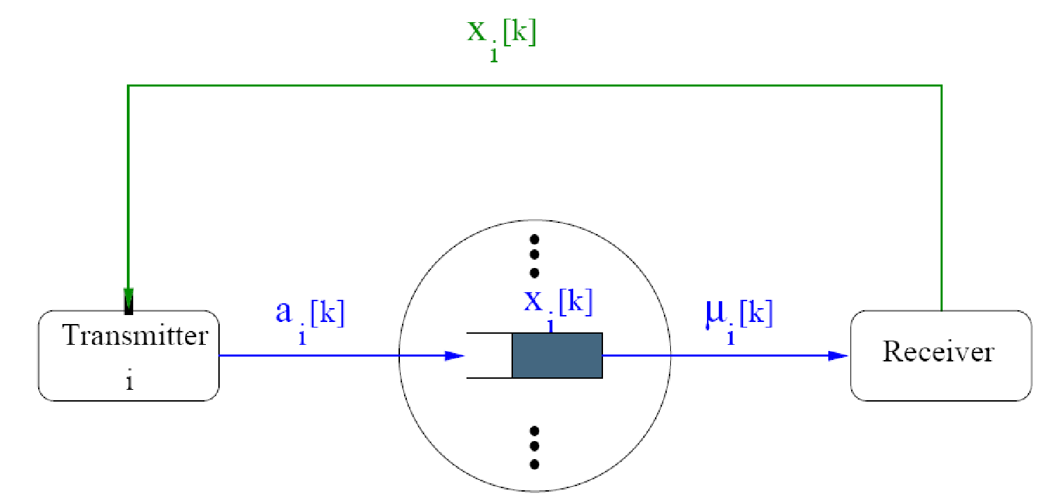

We consider two different scenarios to compare the performance of the greedy policy with the queue-based rate allocation policy by Eryilmaz and Srikant [10]. This policy, parameterized by some parameter , uses queue length information to allocate the rates arbitrarily close to the optimal policy by choosing large enough. As illustrated in Figure 6, denotes the queue-length of the -th user. At time slot , the scheduler chooses the service rate vector based on a max-weight policy, i.e.,
| argmax | (95) | ||||
| subject to |
The congestion controller proposed in [10] leads to a fair allocation of the rates for a given -fair utility function. In particular, the data generation rate for the -th transmitter, denoted by is a random variable satisfying the following conditions:
| (96) |
where , and are positive constants.


In the first scenario, we compare the average achieved rate of the policies for a communication session with limited duration. Figure 7 depicts the distance between empirical average rate achieved by the greedy or the queue-length based policy, and , the maximizer of the utility function over the throughput region. In this case, the utility function is given by (94) with and , and the corresponding optimal solution is . As observed in Figure 7, the greedy policy outperforms the queue-length based policy a communication session with limited duration. It is worth noting that there is a tradeoff in choosing the parameter of the queue-length based policy. In order to guarantee achieving close to optimal rates by queue-based policy, the parameter should be chosen large which results in large expected queue length and lower convergence rate. On the other hand, if takes a small value to improve the convergence rate, the achieved rate of the queue based policy converges to a larger neighborhood of the .
As established in Theorem 5, the performance of the greedy policy improves by decreasing the channel variations. Figure 8 demonstrates the improvement in performance of the greedy policy when decreases from 1.22 to 0.13. We also observe in Figure 8 that the queue-length based policy is not sensitive to channel variations, and its performance does not improve by decreasing the channel variations. It is worth mentioning that the greedy policy as observed in the simulation results performs significantly better than the bounds provided by Theorems 5 and 6. These upper bounds characterize the behavior of the greedy policy in terms of channel variations and structure of the utility function, but they are not necessarily tight.

Second, we consider a file upload scenario where each user transmitting a file with finite size to the base station in a rateless manner. Let be the -th user’s completion time of the file upload session for a file of size . Define the average upload rate for the -th user as . We can measure the performance of each policy for this scenario by evaluating the utility function at the average upload rate. Figure 9 demonstrates the utility difference of the greedy and the queue-based policy for different file sizes. We can observe that for small file sizes the greedy policy outperforms the queue-based policy significantly, and this difference decreases by increasing the file size. We can interpret this behavior as follows. The files are first buffered into the queues based on the queue lengths and the weighted -fair utility, while the queues are emptied by a max-weight scheduler. Once the files are all buffered in the queues, the queues are empties with the same rate which is not fair because it does not give any priority to the users based on their utility. For larger file size, the duration for which the entire file is emptied into the queue is negligible compared to the total transmission time, and the average upload rate converges to a near-optimal rate.
VII Conclusion
We addressed the problem of optimal resource allocation in a fading multiple access channel from an information theoretic point of view. We formulated the problem as a utility maximization problem for a more general class of utility functions.
We considered several different scenarios. First, we considered the problem of optimal rate allocation in a non-fading channel. We presented the notion of approximate projection for the gradient projection method to solve the rate allocation problem in polynomial time in the number of users.
Second, we studied rate and power allocation in a fading channel with known channel statistics. In this case, the optimal rate and power allocation policies are obtained by greedily maximizing a properly defined linear utility function. If for the fading channel power control and channel statistics are not available, the greedy policy is not optimal for nonlinear utility functions. However, we showed that its performance in terms of the utility is not arbitrarily worse compared to the optimal policy, by bounding their performance difference. The provided bound tends to zero as the channel variations become small or the utility function behaves more linearly.
The greedy policy may itself be computationally expensive. A computationally efficient algorithm can be employed to allocate rates close to the ones allocated by the greedy policy. Two different rate allocation policies are presented which only take one iteration of the gradient projection method with approximate projection at each time slot. It is shown that these policies track the greedy policy within a neighborhood which is characterized by average speed of fading as well as fading speed in the worst case.
Appendix A Algorithm for finding a violated constraint
In this section, we present an alternative algorithm based on rate-splitting idea to identify a violated constraint for an infeasible point. For a feasible point, the algorithm provides information for decoding by successive cancellation. We first introduce some definitions.
Definition 11
The quadruple is called a configuration for an -user multiple-access channel, where is the rate tuple, represents the received power and is the noise variance. For any given configuration, the elevation, , is defined as the unique vector satisfying
| (97) |
Intuitively, we can think of message as rectangles of height , raised above the noise level by . In fact, is the amount of additional Gaussian interference that message can tolerate. Note that if the rate vector corresponding to a configuration is feasible its elevation vector is non-negative. However, that is not sufficient for feasibility check.
Definition 12
The configuration is single-user codable, if after possible re-indexing,
| (98) |
where we have defined for convention.
By the graphical representation described earlier, a configuration is single-user codable if the none of the messages are overlapping. Figure 10(a) gives an example of graphical representing for a message with power and elevation . Figures 10(b) and 10(c) illustrate overlapping and non-overlapping configurations, respectively.
Definition 13
The quadruple is a spin-off of if there exists a surjective mapping such that for all we have
where is the set of all that map into by means of .
Definition 14
A hyper-user with power , rate , is obtained by merging actual users with powers and rates , i.e,
| (99) |
Theorem 10
For any -user achievable configuration , there exists a spin-off which is single user codable.
Proof:
See Theorem 1 of [8]. Q.E.D.Here, we give a brief sketch of the proof to give intuition about the algorithm. The proof is by induction on . For a given configuration, if none of the messages are overlapping then the spin-off is trivially equal to the configuration. Otherwise, merge the two overlapping users into a hyper-user of rate and power equal the sum rate and sum power of the overlapping users, respectively. Now the problem is reduced to rate splitting for users. This proof suggests a recursive algorithm for rate-splitting that gives the actual spin-off for a given configuration.
It follows directly from the proof of Proposition 10 that this recursive algorithm gives a single-user codable spin-off for an achievable configuration. If the configuration is not achievable, then the algorithm encounters a hyper-user with negative elevation. At this point the algorithm terminates. Suppose that hyper-user has rate and power . Negative elevation is equivalent to the following
Hence, by Definition 14 we have,
where . Therefore, a hyper-user with negative elevation leads us to a violated constraint in the initial configuration.
Theorem 11
The presented algorithm runs in time, where is the number of users.
Proof:
The computational complexity of the algorithm can be computed as follows. The algorithm terminates after at most recursions. At each recursion, all the elevations corresponding to a configuration with at most hyper-users are computed in time. It takes time to sort the elevation in an increasing order. Once the users are sorted by their elevation, a hyper-user with negative elevation could be found in time, or two if such a hyper-user does not exists it takes time to find two overlapping hyper-users. In the case that there are no overlapping users and all the elevations are non-negative the input configuration is achievable, and the algorithm terminates with no violated constraint. Hence, computational complexity of each recursion is . Therefore, the algorithm runs in time. Q.E.D.

Appendix B Proof of Lemma 5
First, consider the following lemmas. Lemma 9 bounds Jensen’s difference of a random variable for a concave function. The upper bound is characterized in terms of the variance of the random variable.
Lemma 9
Let be concave and twice differentiable. Let be a random variable with variance . Then,
| (100) |
where be an upper-bound on .
Proof:
Pick any . By Chebyshev’s inequality we have
| (101) |
where . Therefore, we have
| (102) | |||||
where the first inequality follows from non-negativity of , and the second and the second inequality follows from concavity of . The scalars and are given by Taylor’s theorem.
Given the above relation, for any we have
| (103) |
The right-hand side is minimized for
| (104) |
By substituting in (103), the desired result follows immediately.
Q.E.D.
We next provide an upper bound on variance of proportional to the variance of .
Lemma 10
Let be a random variable with mean and variance , and then variance of is upper-bounded as
| (105) |
Proof:
Let for some . By invoking the mean value theorem, we have
| (106) | |||||
where is a non-negative random variable.
On the other hand, by employing lemma 9 with , we can write
| (107) |
Hence,
| (108) | |||||
where the first inequality is by (107), and the second relation can be verified after some straightforward manipulation. By combining (106) and (107) the variance of can be bounded as follows
| (109) | |||||
Q.E.D.
Now we provide the proof for Lemma 5. Define random variable as the following:
| (110) |
The facet defining constraints of and are of the form of and , respectively. Therefore, by Definition 6, we have if and only if , for all . Thus, we can write
| (111) | |||||
where the first inequality is obtained by union bound, and the second relation is by applying Chebyshev’s inequality. On the other hand, can be bounded from above by employing Lemma 10, i.e.,
| (112) |
where
Appendix C Proof of Lemma 6
Let us first state and prove a useful lemma which asserts that Euclidean expansion of a capacity region by contains its expansion by relaxing its constraints by .
Lemma 11
Let be a capacity region with polymatroid structure, i.e.,
| (113) |
where is a nondecreasing submodular function. Also, let be an expansion of by as defined in Definition 5. Then, for all , there exists some such that .
Proof:
By Definition 15, it is straightforward to show that is also a polymatroid, i.e.,
| (114) |
where is a submodular function. By convexity of , we just need to prove the claim for the vertices of . Let be a vertex of . The polymatroid structure of implies that is generated by an ordered subset of (see Theorem 2.1 of [32]). Hence, there is some such that . Consider the following construction for :
| (115) |
By construction, is in a -neighborhood of . So we just need to show that is feasible in . First, let us consider the sets that contain . We have
| (116) |
Second, consider the case that .
where the first inequality comes from (116), and the second inequality is true by submodularity of the function . This completes the proof. Q.E.D.
References
- [1] X. Wang and G.B. Giannakis. Energy-efficient resource allocation in time division multiple-access over fading channels. Preprint, 2005.
- [2] S.J. Oh, Z. Danlu, and K.M. Wasserman. Optimal resource allocation in multiservice CDMA networks. IEEE Transactions on Wireless Communications, 2(4):811–821, 2003.
- [3] J.B. Kim and M.L. Honig. Resource allocation for multiple classes of DS-CDMA traffic. IEEE Transactions on Vehicular Technology, 49(2):506–519, 2000.
- [4] J. Huang, V. Subramanian, R. Berry, and R. Agrawal. Joint scheduling and resource allocation in OFDM systems: Algorithms and performance for the uplink. In Proceedings of 41st Annual Asilomar Conference on Signals, Systems, and Computers (invited paper), 2007.
- [5] D. Tse and S. Hanly. Multiaccess fading channels part I: Polymatroid structure, optimal resource allocation and throughput capacities. IEEE Transactions on Information Theory, 44(7):2796–2815, 1998.
- [6] S. Shenker. Fundamental design issues for the future internet. IEEE Journal on Selected Areas in Communications, 13:1176–118, 1995.
- [7] R. Srikant. Mathematics of Internet Congestion Control. Birkhauser, 2004.
- [8] B. Rimoldi and R. Urbanke. A rate-splitting approach to the gaussian multiple-access channel. IEEE Transactions on Information Theory, 42(2):364–375, 1996.
- [9] X. Lin and N. Shroff. The impact of imperfect scheduling on cross-layer rate control in multihop wireless networks. In Proceedings of IEEE Infocom, Miami, FL, March 2005.
- [10] A. Eryilmaz and R. Srikant. Fair resource allocation in wireless networks using queue-length based scheduling and congestion control. In Proceedings of IEEE Infocom, volume 3, pages 1794–1803, Miami, FL, March 2005.
- [11] M.J. Neely, E. Modiano, and C. Li. Fairness and optimal stochastic control for heterogeneous networks. In Proceedings of IEEE Infocom, pages 1723–1734, Miami, FL, March 2005.
- [12] A. Stolyar. Maximizing queueing network utility subject to stability: Greedy primal-dual algorithm. Queueing Systems, 50(4):401–457, 2005.
- [13] A. Eryilmaz, A. Ozdaglar, and E. Modiano. Polynomial complexity algorithms for full utilization of multi-hop wireless networks. In Proceedings of IEEE Infocom, Anchorage, AL, May 2007.
- [14] L. Tassiulas. Linear complexity algorithms for maximum throughput in radio networks and input queued switches. In Proceedings of IEEE Infocom, pages 533–539, 1998.
- [15] E. Modiano, D. Shah, and G. Zussman. Maximizing throughput in wireless networks via gossiping. In ACM SIGMETRICS/IFIP Performance, 2006.
- [16] S. Sanghavi, L. Bui, and R. Srikant. Distributed link scheduling with constant overhead, 2007. Technical Report.
- [17] C. Joo, X. Lin, and N. Shroff. Performance limits of greedy maximal matching in multi-hop wireless networks. In Proceedings of IEEE Conference on Decision and Control, New Orleans LA, December 2007.
- [18] A. Eryilmaz, A. Ozdaglar, D. Shah, and E. Modiano. Randomized algorithms for optimal control of wireless networks, 2007. ICCOPT Conference, Hamilton CA.
- [19] S. Vishwanath, S.A. Jafar, and A. Goldsmith. Optimum power and rate allocation strategies for multiple access fading channels. In Proceedings of IEEE VTC, 2001.
- [20] E. Yeh and A. Cohen. Delay optimal rate allocation in multiaccess fading communications. In Proceedings of the Allerton Conference on Communication, Control, and Computing, Monticello, IL, October 2004.
- [21] D. Yu and J.M. Cioffi. Iterative water-filling for optimal resource allocation in OFDM multiple-access and broadcast channels. In Proceedings of IEEE GLOBECOM, 2006.
- [22] K. Seong, R. Narasimhan, and J. Cioffi. Scheduling for fading multiple access channels with heterogeneous QoS constraints. In Proceedings of International Symposium on Information Theory, 2007.
- [23] H. Liao. Multiple access channels. Ph.D. thesis, University of Hawaii, Honolulu, 1972.
- [24] S. Shamai and A.D. Wyner. Information theoretic considerations for symmetric, cellular, multiple-access fading channels part I. IEEE Transactions on Information Theory, 43(6):1877–1894, 1997.
- [25] D.P. Bertsekas, A. Nedić, and A.E. Ozdaglar. Convex Analysis and Optimization. Athena Scientific, Cambridge, Massachusetts, 2003.
- [26] D.P. Bertsekas. Nonlinear Programming. Athena Scientific, Cambridge, Massachusetts, 1999.
- [27] U. Brännlund. On relaxation methods for nonsmooth convex optimization. Doctoral thesis, Royal Institute of Technology, Stockholm, Sweden, 1993.
- [28] M. Grötschel, L. Lovász, and A. Schrijver. The ellipsoid method and its consequences in combinatorial optimization. Combinatorica, 1(2):169–197, 1981.
- [29] J. Orlin. A faster strongly polynomial time algorithm for submodular function minimization. In Proceedings of the 12th Conference on Integer Programming and Combinatorial Optimization, pages 240–251, 2007.
- [30] A. Nedić and D.P. Bertsekas. Convergence Rate of Incremental Subgradient Algorithms. Stochastic Optimization: Algorithms and Applications (S. Uryasev and P. M. Pardalos, Editors), Kluwer Academic Publishers, 2000.
- [31] R. Gallager. Discrete Stochastic Processes. Kluwer Academic Publishers, London, United Kingdom, 1996.
- [32] R. E. Bixby, W. H. Cunningham, and D. M. Topkis. The partial order of a polymatroid extreme point. Mathematics of Operations Research, 10(3):367–378, 1985.