Dispersive Approach to Abelian Axial Anomaly and $\eta-\eta^{\prime}$ Mixing

The problem of the $\eta\eta^{\prime}$ mixing and particularly the value of the mixing angle $\theta$ has attracted a lot of interest for a long period of time. In the last decade the experimental data significantly improved (see e.g. [1] and references therein). So the improvement of the accuracy of the theoretical prediction of the mixing angle $\theta$ seems to be important. Very rich literature is dedicated to this question (see [2]-[14]).

The well-known estimation, based on Gell-Mann-Okubo mass formulas give the value of $\theta$ about -10^o for a quadratic mass formula and about -23^o for a linear case. Obviously, the accuracy of these estimations is not high.

In the well-known paper [2] many years ago by use of the expansion of the composite operators in the interpolating fields the values of the $\eta\eta^{\prime}\to 2\gamma$ and $J/\psi\to\eta(\eta^{\prime})\gamma$ were considered in the terms of the octet currents. The value of the mixing angle $\theta$ was obtained there by comparison of theoretical results with experimental results (existed at that time). Two possible mechanisms for the pseudoscalar field mixing, offered in [3], so called mass mixing and current-mixing models were discussed, and the values of $\theta$ about $-15^{o}\pm 1.8^{o}$ and $-19.2^{o}\pm 2.2^{o}$ correspondingly were obtained.

The analysis of the axial anomaly generated decays $\eta(\eta^{\prime})\to 2\gamma$ was also performed in [4] (in the framework of ChPT) and [5] and the estimate $\theta$ = $-20^{o}\div 25^{o}$ was obtained. The compehensive general analysis of the pseudoscalar mesons decays by making use of both abelian and nonabelian anomalies was performed in [8]. This approach is based on a standard (differential) form of the anomaly and on the pole approximation.

Another systematic anomaly based approach was developed in [6, 7], where a large set of decay processes was investigated. The mixing angle was estimated as $\theta$ = $-17^{o}\pm 2^{o}$, which significantly differs from the estimation of [8]: $\theta=-9^{o}$ . The possible explanation of such discrepancy is a different role played by the continuum contributions in this two approaches. The significance of the continuum contribution was explicitly mentioned in [7]. It was noted, that for $\eta\eta^{\prime}\to 2\gamma$ decay the value $\theta$ = $-17^{o}\pm 2^{o}$ can be obtained only if one takes into account the continuum contribution which cancel the effects of the large SU(3) breaking (i.e. the ratio $f_{8}/f_{\pi}=1.25$), otherwise the value of $\theta$ grows up to -21^o.

The effect of isoscalar pseudoscalar continuum on the mixing angle was also examined in [11]. In this approach the masses of the isoscalar mesons and their decays were discussed. The value of the mixing angle was estimated in the range $-30.5^{o}<\theta\penalty\ <-18.5^{o}$. The value $-17^{o}<\theta<-13^{o}$ was obtained in [10], where phenomenological analysis of a set of decays was performed.

All the above results were obtained in the mixing scheme with one angle. The case of the two mixing angles [16, 12, 13, 14] we will discuss in the section 4.

We can see that all results are compatible , but with relatively large uncertainties.

That’s why it seems reasonable, and this is the main aim of this paper, to use the dispersion form of axial anomaly to find some model-independent and precise restriction on the value of the mixing angle. We will develop the method, used in [23], where a very precise prediction on $\pi^{0}\to 2\gamma$ decay was obtained.

In section 3 we will discuss the one angle octet-singlet mixing scheme and a very precise restrictions will be obtained. The scheme with two angles will be discussed in sect. 4.

Consider a matrix element for a transition of the 8th component of the axial current into two photons with momenta $p$, $p^{\prime}$ and polarizations $\epsilon_{\alpha}$ , $\epsilon^{\prime}_{\beta}$:

where

Here $u$, $d$ and $s$ are fields of u,d and s respective quarks.
We are interested in the decay into two real photons, thus the general form of $T_{\mu\alpha\beta}(p,p^{\prime})$ can be expressed as:

where $q=p+p^{\prime}$.

Using the dispersive approach [17] (see also [21] and references therein) one can derive the exact ”anomaly sum rule” [18, 19, 20] :

where $e_{u}=2/3$,  $e_{d}=e_{s}=1/3$ are electric charges of $u$, $d$, and $s$ quarks, $N_{c}=3$ (the number of colors).

Notice, that in QCD this equation does’t have any perturbative corrections [22], and it is expected that it does not have any nonperturbative corrections as well due to t’Hooft’s consistency principle[19]. It is also important that at $q^{2}\to\infty$ the function $ImF_{1}(q^{2})$ decreases as $1/q^{4}$.

Based on the dispersion relation (4) for an axial anomaly, a high precision prediction for $\pi^{0}\rightarrow 2\gamma$ decay was obtained [23] ( 1.5% , mixing $\pi^{0}$ - $\eta$ was taken into account) and later was confirmed by experiment.

Let us first try to saturate the above relation by the $\eta$ contribution only. We use the following standard definition of the $\eta$ decay constant:

The general form of the $\eta$-contribution to $T_{\mu\alpha\beta}(p,p^{\prime})$ can be written as:

where $\widetilde{A}_{\eta}$ is a constant. So we see, that in the naive approximation, when only $\eta$ contribution is accounted in the l.h.s. of the sum rule for anomaly relation (4), one can find $\widetilde{A}_{\eta}$

Then one can easily calculate the decay width $\eta\rightarrow 2\gamma$ [21]:

If we substitute experimental numbers of $\alpha$, $m_{\eta}$ and $f_{\eta}=1.2f_{\pi}\approx 150MeV$ we’ll get the numerical value

which is in a striking contradiction with an experimental value

Such a large contradiction with exact anomaly dispersion relation motivates us to consider the effects arising from the other states contributions to the sum rule. We will mainly discuss the mixing of $\eta$ and $\eta^{\prime}$ mesons, because calculation show, that effect of $\pi-\eta$ mixing is found to be extremely small. We will say a few words about this later.

Let us now consider the decay $\eta\rightarrow 2\gamma$ using the dispersive approach and taking into account mixing of $\eta$ and $\eta^{\prime}$ mesons. We start with the well-known octet-singlet mixing scheme.

Following [24, 25], let’s introduce nonorthogonal states $|P_{8}\rangle$ and $|P_{0}\rangle$ and the corresponding fields $\varphi_{8}$, $\varphi_{0}$, coupled to $J^{(8)}_{\mu 5}$ and $J^{(0)}_{\mu 5}$:

Nonorthogonality of the fields $\varphi_{8}$, $\varphi_{0}$ corresponds to the non-diagonal term $\Delta H=m^{2}_{\eta\eta^{\prime}}\varphi_{8}\varphi_{0}$ in the effective interaction Hamiltonian. In the presence of such term the standard PCAC relation is modified in the following way:

The fields $\varphi_{8}$,$\varphi_{0}$ are expressed through the physical fields $\varphi_{\eta}$, $\varphi_{\eta^{\prime}}$ as

Mixing angle $\theta$ can be expressed from (9),(10) in terms of masses as:

Now $ImF_{1}(q^{2})$ is given by the sum of contributions of $\eta$ and $\eta^{\prime}$ mesons. In order to separate the formfactor $F_{1}(q^{2})$, multiply $T_{\mu\alpha\beta}(p,p^{\prime})$ by $q_{\mu}/q^{2}$. Then, taking the imagenary part of $F_{1}(q^{2})$, we get:

where $A_{\eta}$ ( $A_{\eta^{\prime}}$) is the amplitude of decay $\eta(\eta^{\prime})\to 2\gamma$.

If we employ sum rule (4), we obtain:

Now let’s express amplitudes in terms of decay widths, employ the relation (11) for a mixing parameter $m_{\eta\eta^{\prime}}^{2}$ and finally get the equation for a mixing angle $\theta$:

where the dimensionless parameters $\beta$ and $\xi$ were introduced:

Before starting a numerical analysis, let us discuss the accuracy of the obtained equation and possible additional contributions. The other (besides $\eta$ and $\eta^{\prime}$) pseudoscalar meson states contributions can arise as some additional terms in the r.h.s of eq.(12). But due to the fact, that $ImF_{1}$ decrease as $1/q^{4}$ at large $q^{2}$, from dimensional ground one can easily conclude, that higher resonances contribution should be suppressed significantly stronger than $(m_{\eta}/m_{res})^{2}$, more probably as a fourth power of the mass ratio. This fact effectively suppresses uncontrolled contributions of higher resonances and continuum and, consequently, allow us to reach a higher accuracy. This is one of the advantages of this method. The numerical analysis show, that possible influence of this uncontrolled effects on the solution of the eq. (14) (i.e. mixing angle $\theta$) is very small (at a few per cent level).

We also calculated the contribution of the $\pi-\eta$ mixing effects in the same way (in fact all what is necessary for this was done in [23]). The pion mixing contribution was found to be extremely small (less than a per cent, suppressed as $(m_{\pi}/m_{\eta})^{4}$), that’s why we don’t mention it.

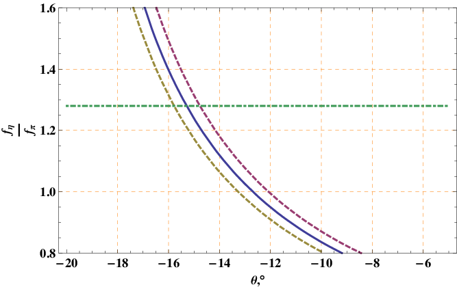
For a numerical analysis of our anomaly sum rule equation (14) we use the following experimental data (PDG Review 2008) [26]: $m_{\eta}=547.853\pm 0.024$ MeV, $m_{\eta^{\prime}}=957.78\pm 0.24$ MeV,  $\Gamma_{\eta\to 2\gamma}=0.510\pm 0.026$ keV,  $\Gamma_{\eta^{\prime}\to 2\gamma}=4.30\pm 0.15$ keV.  Also for a convenience we will present $f_{\eta}$ in units of a decay constant of pion $f_{\pi}=130.7$ MeV. The only parameter in eq. (14) that has no a well-defined experimental value, is $f_{\eta}$. If we use a well established prediction of ChPT (see e.g. [15]) $f_{\eta}=1.28f_{\pi}$, we get:

Error bars include both theoretical and experimental uncertainties which happened of the same order. It is useful to express $f_{\eta}$ from eq. (14) as a function of $\theta$. Remarkably, the function $f_{\eta}(\theta)$ within the interval of reasonable values of $f_{\eta}$ shows quite strong dependence on the mixing angle $\theta$ (fig.1). Moreover, expression (14) manifests also a dramatic dependence of the width $\Gamma_{\eta}\to 2\gamma$ on the mixing angle $\theta$. This property of the anomaly motivated equations (12), (14) explains how the relatively small mixing strongly effects the decay width.

It is interesting also to note, that eq. (14) as an equation for $\theta$ formally has 6 roots for $f_{\eta}\gtrsim 0.5f_{\pi}$ and only 4 roots for $f_{\eta}\lesssim 0.5f_{\pi}$ (see fig.2). Moreover, the only physical root is among these two disappearing roots.

An approach with one mixing angle in study of $\eta-\eta^{\prime}$ system dominated for decades. But in the recent years there was a rise of interest to the mixing scheme with two angles. It was noticed that taking into account the chiral anomaly through perturbative expansion in ChPT can lead to the introduction of two mixing angles in description of the $\eta$- $\eta^{\prime}$ system [16]. There were also performed some phenomenological analysis of various decay processes in the approach of two angle mixing scheme [12, 14].

In this section we will consider a two angle mixing scheme for the $\eta-\eta^{\prime}$ system using the approach developed in the previous section. We suggest a straightforward generalization of approach [24, 25] by combining PCAC relation (8) with presence of two mixing angles $\theta_{1}$ and $\theta_{2}$ (cf. [12] ):

When mixing angles $\theta_{1}$ and $\theta_{2}$ are equal to each other, one comes back to the scheme with one mixing angle. The anomaly sum rule equation for a two angle mixing scheme now reads:

where $\beta$ and $\xi$ are defined by (15) and

If we use the experimental values for masses $m_{\eta}$, $m_{\eta^{\prime}}$ and widths $\Gamma_{\eta\to 2\gamma}$, $\Gamma_{\eta^{\prime}\to 2\gamma}$ as in the previous section, we will get the equation which contains as parameters angles $\theta_{1}$, $\theta_{2}$ and $f_{\eta}$. For physically interesting values of angles we get the plot shown on the fig.3. The resulting plot for a full space of parameters is presented on the fig.4. We may see that the angles play rather different role. While $\theta_{1}$ is tightly bounded by the data, like in the case of one angle mixing scheme, the sensitivity ro the changes of $\theta_{2}$ is rather weak.

It was shown that the use of dispersive representation of electromagnetic axial anomaly leads to tight bounds for the $\eta-\eta^{\prime}$ mixing angle: $\theta=-15.3^{\circ}\pm 1^{\circ}$. This is model independent precise prediction which should be taken into account in future analyses.

One of the main advantages of this method is effective suppression of the higher contribution and higher resonances which are usually the main source of uncertainties.

Moreover, our result manifests also a dramatic dependence of the width $\Gamma_{\eta\to 2\gamma}$ on the mixing angle $\theta$. This property explains how the relatively small mixing strongly effects the decay width.

We considered also two angle mixing scheme and and found that rather weakly correlated: while the first angle is still tightly bounded, the second one may vary in a rather wide region.

The authors thank D.I. Dyakonov, A.V. Efremov, G. t’Hooft, B.L. Ioffe and A.V. Kisselev for useful discussions and comments. This work was supported in part by the Russian Foundation of Basic Research, projects no. 06-02-16905a, 06-02-16215a, 07-02-91557, 08-02-00896a and the funds from EC to the project ”Study of the Strong Interacting Matter” under contract N0. R113-CT-2004-506078.

References

- [1] C. E. Thomas, JHEP 0710, 026 (2007) [arXiv:0705.1500 [hep-ph]].
- [2] A.V. Kisselev and V.A. Petrov, Z. Phys. C58, 595-600 (1993)
- [3] N. M. Kroll, T. D. Lee and B. Zumino, Phys. Rev. 157, 1376 (1967).
- [4] J. F. Donoghue, B. R. Holstein and Y. C. R. Lin, Phys. Rev. Lett. 55, 2766 (1985) [Erratum-ibid. 61, 1527 (1988)].
- [5] F. J. Gilman and R. Kauffman, Phys. Rev. D 36, 2761 (1987) [Erratum-ibid. D 37, 3348 (1988)].
- [6] R. Akhoury and J. M. Frere, Phys. Lett. B 220, 258 (1989).
- [7] P. Ball, J. M. Frere and M. Tytgat, Phys. Lett. B 365, 367 (1996) [arXiv:hep-ph/9508359].
- [8] D. Diakonov and M. I. Eides, Sov. Phys. JETP 54, 232 (1981) [Zh. Eksp. Teor. Fiz. 81, 434 (1981)].
- [9] T. N. Pham, Phys. Lett. B 246, 175 (1990).
- [10] R. Escribano and J. M. Frere, Phys. Lett. B 459, 288 (1999) [arXiv:hep-ph/9901405].
- [11] N. F. Nasrallah, Phys. Rev. D 70, 116001 (2004) [Erratum-ibid. D 72, 019903 (2005)] [arXiv:hep-ph/0410240].
- [12] T. Feldmann, P. Kroll and B. Stech, Phys. Rev. D 58, 114006 (1998) [arXiv:hep-ph/9802409].
- [13] P. Kroll, Mod. Phys. Lett. A 20, 2667 (2005) [arXiv:hep-ph/0509031].
- [14] R. Escribano and J. M. Frere, JHEP 0506, 029 (2005) [arXiv:hep-ph/0501072].
- [15] R. Kaiser and H. Leutwyler, arXiv:hep-ph/9806336.
- [16] H. Leutwyler, Nucl. Phys. Proc. Suppl. 64, 223 (1998) [arXiv:hep-ph/9709408].
- [17] A. D. Dolgov and V. I. Zakharov, Nucl. Phys. B 27, 525 (1971).
- [18] J. Horejsi, Phys. Rev. D 32, 1029 (1985).
- [19] J. Horejsi and O. Teryaev, Z. Phys. C 65, 691 (1995).
- [20] O. L. Veretin and O. V. Teryaev, Yad. Fiz. 58, 2266 (1995)
- [21] B. L. Ioffe, Int. J. Mod. Phys. A 21, 6249 (2006) [arXiv:hep-ph/0611026].
- [22] S. L. Adler and W. A. Bardeen, Phys. Rev. 182, 1517 (1969).
- [23] B. L. Ioffe and A. G. Oganesian, Phys. Lett. B 647, 389 (2007) [arXiv:hep-ph/0701077].
- [24] B. L. Ioffe, Yad. Fiz. 29, 1611 (1979).
- [25] B. L. Ioffe and M. A. Shifman, Phys. Lett. B 95, 99 (1980).
- [26] C. Amsler et al. [Particle Data Group], Phys. Lett. B 667, 1 (2008).