Simulation of Laser Beam Propagation With a Paraxial Model in a Tilted Frame

Marie Doumic ^†^†thanks: Corresponding author M. Doumic: marie.doumic@inria.fr^†^†thanks: I.N.R.I.A Rocquencourt, BANG project, Domaine de Voluceau, B.P. 105, 78153 Rocquencourt, France, marie.doumic@inria.fr Frédéric Duboc ^†^†thanks: CEA/Bruyères, B.P. 12, 91680 Bruyères-Le-Chatel, France, frederic.duboc@cea.fr François Golse ^†^†thanks: Ecole Polytechnique, Centre de Mathématiques Laurent Schwartz, 91128 Palaiseau Cedex, France, golse@math.polytechnique.fr Rémi Sentis ^†^†thanks: CEA/Bruyères, B.P. 12, 91680 Bruyères-Le-Chatel, France, remi.sentis@cea.fr

Abstract

We study the Schrödinger equation which comes from the paraxial approximation of the Helmholtz equation in the case where the direction of propagation is tilted with respect to the boundary of the domain. In a first part, a mathematical analysis is made which leads to an analytical formula of the solution in the simple case where the refraction index and the absorption coefficients are constant. Afterwards, we propose a numerical method for solving the initial problem which uses the previous analytical expression. Numerical results are presented. We also sketch an extension to a time dependant model which is relevant for laser plasma interaction.

1 Introduction

For the simulation of the propagation of a monochromatic laser beam in a medium where the local refractive index is nearby a constant, it is classical to use the paraxial approximation of the Maxwell equations. This approximation takes into account diffraction and refraction phenomena ; it is intensively used for decades in optics and in a lot of models related to laser-plasma interaction in Inertial Confinement Fusion experiments (cf [4],[10], [21], [14] and the bibliography of these references). Let us first recall briefly the outlines of this approximation. Denote by $2\pi\epsilon$ the laser wave-length, it is in the order of 1 $\mu m$ and is very small compared to the characteristic length of the simulation domain (which is in the order of some $mm$ for the Inertial Confinement plasmas). According to laws of optics, the laser electromagnetic field may be modeled by the solution $\psi$ of the following Helmholtz equation (which comes from the time envelope of the full Maxwell equations):

\epsilon^{2}{\Delta}\psi+\psi+2i\epsilon\nu_{t}\psi=0,

(1)

where we have denoted:

\nu_{t}(\mathbf{x})=\nu(\mathbf{x})+i\mu(\mathbf{x}),

so $\nu_{t}$ is a complex function, its real part $\nu$ corresponds to a conveniently scaled absorption coefficient and its imaginary part $\mu$ to the variation of the refractive index ( $1-2\epsilon\mu$ is equal to the square of the refractive index $n$ up to a multiplicative constant).

We assume also that the light propagates according a fixed direction defined by the unit vector $\mathbf{k}.$ After making the classical WKB expansion:

\psi=u\exp(\frac{i\mathbf{k}.\mathbf{x}}{\epsilon}),

(2)

equation (1) may read as $2i\nu_{t}u+2i\mathbf{k}.{\mathbf{\nabla}}u+\epsilon\Delta_{\bot}u=\epsilon(\mathbf{k}.{\mathbf{\nabla}})^{2}u,$ where $\Delta_{\bot}$ is the Laplace operator with respect to the transverse variable:

\Delta_{\bot}\bullet=\nabla.[(\mathbf{1}-\mathbf{k}\otimes\mathbf{k})\nabla\bullet],\quad\mathbf{1}\hbox{ being the unit diagonal tensor.}

Assuming that $u$ is slowly varying with respect to the longitudinal variable, we can neglect the right hand side of the previous equation. Therefore $u$ satisfies the classical paraxial equation for wave propagation:

i\mathbf{k}.\nabla u+\frac{\epsilon}{2}\Delta_{\bot}u+i\nu_{t}u=0,\qquad{\rm with}\quad\nu_{t}=\nu+i\mu.

(3)

For this kind of model, it is usual to handle a simulation box which is a parallelepiped and the laser beam is assumed to enter into the simulation box on a plane boundary denoted by $\Gamma_{0}.$ Let us denote $\mathbf{n}$ the outward normal vector to the incoming boundary $\Gamma_{0}.$ Classically, the crucial assumption is that the laser beam enters into the simulation domain with a very small incidence angle, that is to say the vector $\mathbf{k}$ is almost equal to $-\mathbf{n}$ . Then, in such a framework, (3) is a classical linear Schrödinger equation, the operator $\mathbf{k}.\nabla$ plays the part of time derivative and the boundary condition on $\Gamma_{0}$ which reads $u=u^{in}\$ (where $u^{in}$ is a given function defined on $\Gamma_{0}$ ) plays the part of the initial condition. On the other hand, artificial absorbing boundary conditions are to be imposed on the faces of the simulation domain parallel to the vector $\mathbf{k},$ (see for example [1], [7], [15]). The numerical methods are always implemented on an orthogonal mesh and are based on a splitting with respect to the main spatial variable between the diffraction part $(\frac{\epsilon}{2}\Delta_{\bot}u)$ and refraction part $(i\nu_{t}u),$ see [4], [3], [10] for example.

We address in this paper a different case where the incidence angle of $\mathbf{k}$ with $-\mathbf{n}$ is large; these simulations are called tilted frame simulations. This kind of simulations is of particular interest if one has to deal with the crossing between two beams (in the high energy laser devices, a large number of beams are focused on the target, therefore beam crossing may be taken into account, see [8] for a survey on related laser propagation problems); an example of such simulations in a very simplified case may be found on Figure 13. This tilted frame model has been considered some years ago by physicists for dealing with beam crossing problems (see [20]).

Simulations in a tilted frame are also necessary for dealing with special situations. For instance for the propagation of a beam in a domain where the profile of the refractive index $n$ is such that $n^{2}(\mathbf{x})=n_{0}^{2}(1-\varepsilon\mu(\mathbf{x}))$ (with $n_{0}$ constant smaller than 1) in a first subdomain $\mathcal{D}$ and $n^{2}(\mathbf{x})=\mathcal{N}(\mathbf{x}.\mathbf{n}^{\ast})+\delta\mathcal{N}(\mathbf{x})$ (where $\mathcal{N}\in[0,n_{0}]$ depends on a one-dimension variable $\mathbf{x}.\mathbf{n}^{\ast}$ and $\delta\mathcal{N}$ is small with respect to $1$ ) in a second juxtaposed subdomain $\mathcal{D}^{H}$ , one must handle the paraxial equation (3) in subdomain $\mathcal{D}$ and the Helmholtz equation (1) in subdomain $\mathcal{D}^{H}$ . For the numerical solution of (1), one has to solve a huge linear system (corresponding to the discretization of the equation on a very fine grid) and for handling this huge linear system, it is necessary that the variable $\mathbf{x}.\mathbf{n}^{\ast}$ corresponds to one of the main direction of $\mathcal{D}^{H}$ . Therefore the full simulation on $(\mathcal{D}\cup\mathcal{D}^{H})$ has to be performed in a box such that the corresponding normal vector $\mathbf{n}$ must be parallel to $\mathbf{n}^{\ast}$ (see [6] for details for this kind of simulations).

In the case of a large incidence angle, the crude expansion $\psi=U\exp({-i\mathbf{n}.\mathbf{x}}/{\epsilon})$ leads to difficulties and to overcome these difficulties, it has been proposed in [13] to replace the transverse Laplacian by a pseudodifferential operator, but with this approximation, $U$ is not slowly varying with respect to the spatial coordinates therefore it is necessary to handle very fine mesh -at least 10 cells per wave length- to get accurate results. One can also refer to the works in the spirit of [16] in the acoustic framework but the application to the optics problems seems to be difficult.

Here we consider the expansion $\psi=u\exp({i\mathbf{k}.\mathbf{x}}/{\epsilon}),$ with $u$ slowly varying with respect to $\mathbf{k}.\mathbf{x,}$ so we have to deal with the tilted frame Laplace operator $\Delta_{\bot}$ and one has to supplement the equation (3) with a right incoming boundary condition on $\Gamma_{0}$ . For the statement of this boundary condition, one assumes that a fixed plane wave $\psi^{in}=u^{in}\exp(i\mathbf{k}.\mathbf{x}/{\epsilon})$ enters into the domain where $u^{in}$ is a given function of the variable which is orthogonal to $\mathbf{k}.$ Now, for the Helmholtz problem, the boundary condition is classical and may be written as $(\epsilon\mathbf{n}.\nabla+i\mathbf{k}.\mathbf{n})(\psi-u^{in}e^{i\mathbf{k}.\mathbf{x}\mathbf{/\epsilon}})=0,$ then using (2) and an asymptotic expansion with respect to the small parameter ${\epsilon}$ , the corresponding boundary condition for equation (3) may read in a natural way as:

(\epsilon\mathbf{n}.\nabla_{\bot}+2i\mathbf{k}.\mathbf{n})(u-u^{in})=0,

(4)

where $\nabla_{\bot}=\nabla-\mathbf{k}(\mathbf{k}.\nabla)$ denotes the gradient orthogonal to $\mathbf{k}.$ See [9] for a justification of the paraxial approximation in the special case we are dealing with.

If one sets $\mathbf{x}=(x,y,z)$ in 3D and $\mathbf{x}=(x,y)$ in 2D, the entrance boundary $\Gamma_{0}$ corresponds in this paper to $x=0$ . In the sequel we consider a 2D problem but most of the ideas of this work may be extended to the 3D case.

Equation (3) may be recast as:

i(k_{x}\partial_{x}u+k_{y}\partial_{y}u)+\frac{\epsilon}{2}\Delta_{\bot}u+i\nu_{t}u=0,

and up to our knowledge, the numerical solution of this kind of equations is novel; the main difficulty is to handle correctly the tilted Laplace operator $\Delta_{\bot}u$ . For the mathematical analysis of the problem, one key result is the following (cf. proposition 2). On the half-space $\{(x,y)\quad\mathrm{s.t.}\quad x\geq 0\},$ if the coefficient $\nu_{t}$ is a positive real constant, after taking the Fourier transform with respect to the $y$ variable, the problem (3)(4) is equivalent to an ordinary differential equation with respect to the $x$ variable and it is possible to exhibit an analytical solution. This analytical formula is the convenient tool for numerical treatment of the diffraction part of (3) in the general case where $\nu_{t}$ is not constant.

The paper is organized as follows. In Section 2, after setting classical energy estimates for Problem (3) supplemented by (4), we prove the above mentioned theoretical result.

Section 3 is devoted to the description of the numerical scheme for solving Problem (3)(4) ; it is based on a splitting method with respect to the spatial variable $x$ using fast Fourier transforms on a first step (for the diffraction part) and a standard finite difference method on a second step (for the advection and refraction part).

In Section 4, we give the numerical results on the initial problem and for a model where the coefficient $\mu$ in (3) is replaced by $f(|u|)$ corresponding to the autofocusing which occurs in the laser-plasma interaction (see [19] for instance). From a physical point of view, this term represents a variation of the plasma electronic density caused by the ponderomotrice force of the laser. In the last section we consider a more general model where the stationary problem (3) is replaced by a time dependent one which is coupled to a hydrodynamic system for a suitable modeling of the plasma behavior.

2 Analysis of the Tilted Paraxial Equation

For reasons which will appear in the sequel, we assume in this section that

\hbox{inf}_{\mathbf{x}}\nu(\mathbf{x})>0.

(5)

We first study the problem where the simulation domain is the half-space:

{\cal D}=\big\{\mathbf{x}=(x,y)\quad{\rm s.t.}\quad x>0\big\},\quad\Gamma_{0}=\big\{\mathbf{x}=(0,y)\big\}.

Assuming that $\mu$ is a bounded function, we consider the following problem:

	$\displaystyle i\mathbf{k}\cdot\mathbf{\mathbf{\nabla}}u+\frac{\epsilon}{2}\Delta_{\bot}u-\mu u+i\nu u=0\qquad{\rm on}\;{\cal D},$		(6)
	$\displaystyle(i\epsilon\mathbf{n}.\nabla_{\bot}-2\mathbf{k}.\mathbf{n})(u-u^{in})=0\qquad{\rm on}\;\Gamma_{0}.$		(7)

2.1 Energy Estimate

Let us first state the following classical estimate.

Proposition 1

Let $(i\epsilon\mathbf{n}.\nabla_{\bot}-2\mathbf{k}.\mathbf{n})u^{in}\in L^{2}(\mathds{R})$ . If $u\in H^{1}({\cal D})$ is a solution to Problem (6) (7), it is unique. Moreover, we have the following stability estimate, with a constant $C$ independent of $\nu,$ $\mu$ :

\iint\limits_{\mathcal{D}}2\nu|u|^{2}+\int\limits_{\Gamma_{0}}|\mathbf{k}\cdot\mathbf{n}||u|^{2}dy\leq C\int\limits_{\Gamma_{0}}|(i\epsilon\mathbf{n}.\nabla_{\bot}-2\mathbf{k}.\mathbf{n})u^{in}|^{2}dy.

Proof. Let us denote $D=\mathbf{n}.\nabla_{\bot}$ . Doing the scalar product of Equation (3) with $u$ and taking its imaginary part, we get:

\int\limits_{\Gamma_{0}}\biggl(|u|^{2}\mathbf{k}\cdot\mathbf{n}+\frac{\epsilon}{2i}(\bar{u}Du-uD\bar{u})\biggr)dy+\iint\limits_{\cal D}2\nu|u|^{2}d\mathbf{x}=0.

According to the boundary condition (7) we check that:

\frac{\epsilon}{2i}(\bar{u}Du-uD\bar{u})=-2\mathbf{k}\cdot\mathbf{n}|u|^{2}+{\cal I}m\bigl(\bar{u}(\epsilon D+2i\mathbf{k}\cdot\mathbf{n})u^{in}\bigr).

Then we get:

\iint\limits_{\mathcal{D}}2\nu|u|^{2}d\mathbf{x}+\int\limits_{\Gamma_{0}}|\mathbf{k}.\mathbf{n}||u|^{2}dy=-{\cal I}m\bigl(\int\limits_{\Gamma_{0}}\bar{u}(\epsilon D+2i\mathbf{k}.\mathbf{n}){u^{in}}dy\bigr).

(8)

According to (8), if $(i\epsilon D-2\mathbf{k}\cdot\mathbf{n})u^{in}=0,$ we see that $\iint\limits_{\mathcal{D}}2\nu|u|^{2}d\mathbf{x}=0,$ so $u=0.$ Therefore we get the uniqueness of the solution of Problem (6)(7).

To obtain the stability inequality, we first see that Equation (8) implies:

|\mathbf{k}\cdot\mathbf{n}|\int\limits_{\Gamma_{0}}|u|^{2}\leq\sqrt{\int\limits_{\Gamma_{0}}|u|^{2}}\sqrt{\int\limits_{\Gamma_{0}}|(\epsilon D+2i\mathbf{k}\cdot\mathbf{n}){u^{in}}|^{2}}.

Using this estimate, Equation (8) leads to:

\iint\limits_{\mathcal{D}}2\nu|u|^{2}d\mathbf{x}+\int\limits_{\Gamma_{0}}|\mathbf{k}\cdot\mathbf{n}||u|^{2}\leq\sqrt{\int\limits_{\Gamma_{0}}|u|^{2}}\sqrt{\int\limits_{\Gamma_{0}}|(\epsilon D+2i\mathbf{k}\cdot\mathbf{n}){u^{in}}|^{2}}\leq\frac{1}{|\mathbf{k}\cdot\mathbf{n}|}\int\limits_{\Gamma_{0}}|(\epsilon D+2i\mathbf{k}\cdot\mathbf{n}){u^{in}}|^{2}.

$\diamondsuit$

By the same technique we get also the following estimate:

\iint\limits_{\mathcal{D}}2\nu|u|^{2}+\int\limits_{\Gamma_{0}}\frac{|\mathbf{k}.\mathbf{n}|}{2}|\frac{(i\epsilon D+2\mathbf{k}.\mathbf{n})u}{2|\mathbf{k}.\mathbf{n}|}|^{2}=\int\limits_{\Gamma_{0}}|\mathbf{k}.\mathbf{n}|\biggl(|u|^{2}+\frac{1}{2}|\frac{(i\epsilon D-2\mathbf{k}.\mathbf{n})u^{in}}{2|\mathbf{k}.\mathbf{n}|}|^{2}\biggr),

which says that the absorbing energy plus the the outgoing energy is equal to the incoming energy.

2.2 Analytical Form of the Solution in the Case $\nu_{t}$ Constant

We now assume that $\mu=0$ and $\nu$ is constant for getting an analytical form of the solution to Problem (3)(4). We denote $\mathbf{k}=(k_{x},k_{y})$ and $g$ the function defined by:

2k_{x}g=i\epsilon k_{y}(k_{x}{\partial_{y}}-k_{y}{\partial_{x}})u^{in}+2k_{x}u^{in}.

(9)

The problem may read as:

	$\displaystyle i(k_{x}{\partial_{x}}+k_{y}{\partial_{y}})u+\frac{\epsilon}{2}(k_{x}^{2}{\partial^{2}_{yy}}-2k_{x}k_{y}{\partial^{2}_{xy}}+k_{y}^{2}{\partial^{2}_{xx}})u+i\nu u=0,\qquad{\rm on}\;\cal{D},$		(10)
	$\displaystyle i\epsilon k_{y}(k_{x}{\partial_{y}}-k_{y}{\partial_{x}})u+2k_{x}u=2k_{x}g,\qquad\;{\rm on}\Gamma_{0}.$		(11)

In the sequel, the Fourier variables related to $x$ and $y$ respectively are $\xi$ and $\eta.$ The Fourier transform in $x$ and $y$ are denoted by ${\cal F}_{x}(\bullet)$ and ${\cal F}_{y}(\bullet)$ , moreover ${\cal F}_{y}(u;x,.)$ denotes the Fourier transform of $u(x,.)$ .

Here and in the sequel, $\sqrt{\penalty\ \penalty\ }$ denotes the principal determination of the square root (its real part is positive). Denote:

R_{-}(i\eta)=i\frac{k_{x}\eta}{k_{y}}-i\frac{k_{x}}{{\epsilon k_{y}^{2}}}(1-\sqrt{1-2\frac{\epsilon k_{y}\eta}{k_{x}^{2}}+2i\nu\frac{\epsilon k_{y}^{2}}{k_{x}^{2}}}).

Since $\nu>0,$ one can define $R_{-}$ without ambiguity and one checks that ${\cal R}e(R_{-}(i\eta))<0$ for all $\eta.$ Let ${\cal S}^{\prime}(\mathds{R})$ be the space of tempered distributions.

Proposition 2

Assume that $g\in{\cal S}^{\prime}(\mathds{R}),$ then there exists a unique distribution $u(x,.)$ continuous from $\mathds{R}^{+}$ into ${\cal S}^{\prime}_{y}(\mathds{R}),$ solution to Problem (10)(11). It is given by:

{\cal F}_{y}(u;x,\eta)=\frac{2{\cal F}_{y}(g;\eta)}{1+\sqrt{1-2\frac{\epsilon k_{y}\eta}{k_{x}^{2}}+2i\nu\frac{\epsilon k_{y}^{2}}{k_{x}^{2}}}}e^{R_{-}(i\eta)x}.

(12)

It satisfies also:

\biggl({\partial_{x}}-R_{-}(i\eta)\biggr){\cal F}_{y}(u;x,\eta)=0.

Proof.

The principle is to take the Fourier transform in $y$ of the problem, and afterwards we shall consider Fourier transform in $x$ of the equation extended to the whole space.

Let $u$ be a solution of Problem (10)(11) and $v$ the extension of $u$ by zero in the whole space: $v(x,y)=u(x,y){{\mathds{1}}}_{x\geq 0}$ . By introducing formally the function $v$ in Equation (10) we get:

i\mathbf{k}\cdot\mathbf{\mathbf{\nabla}}v+\frac{\epsilon}{2}\Delta_{\bot}v+i\nu v=\biggl(\bigl(ik_{x}-\frac{\epsilon k_{y}}{2}(2k_{x}{\partial_{y}}-k_{y}{\partial_{x}})\bigr)u(0,y)\biggl){\delta}_{x=0}+\frac{\epsilon k_{y}^{2}}{2}u(0,y){\delta}^{{}^{\prime}}_{x=0}.

The term ${\partial_{x}}u(0,y)$ is defined by the entrance boundary condition (11), so we get:

i\mathbf{k}\cdot\mathbf{\mathbf{\nabla}}v+\frac{\epsilon}{2}\Delta_{\bot}v+i\nu v=ik_{x}g(y)\delta_{x=0}-\frac{\epsilon k_{y}}{2}\bigl(k_{x}{\partial_{y}}u(0,y){\delta}_{x=0}-k_{y}u(0,y){\delta}^{{}^{\prime}}_{x=0}\bigr).

Assuming that $u\in{\cal C}(\mathds{R}_{+},{\cal S}^{\prime}(\mathds{R}))$ , we are allowed to take the Fourier transform of this expression. Let us define $P(X,Y)$ as the polynomial which characterizes the differential operator of the equation, that is to say:

P({\partial_{x}},{\partial_{y}})=i(k_{x}{\partial_{x}}+k_{y}{\partial_{y}})+\frac{\epsilon}{2}(k_{y}^{2}{\partial^{2}_{xx}}-2k_{x}k_{y}{\partial^{2}_{xy}}+k_{x}^{2}{\partial^{2}_{yy}})+i\nu.

Writing $u_{0}(y)=u(0,y)$ , the Fourier transform in $y$ of the equation in $v$ reads:

P({\partial_{x}},i\eta){\cal F}_{y}(v;x,\eta)=\frac{\epsilon k_{y}^{2}}{2}\biggl\{\biggl(\frac{2ik_{x}}{\epsilon k_{y}^{2}}{\cal F}_{y}(g;\eta)-i\frac{k_{x}}{k_{y}}\eta{\cal F}_{y}(u_{0};\eta)\biggr)\delta_{x=0}+{\cal F}_{y}(u_{0};\eta)\delta^{{}^{\prime}}_{x=0}\biggr\}.

Polynomial $P$ may be factorized as:

P({\partial_{x}},i\eta)=\frac{\epsilon k_{y}^{2}}{2}\biggl({\partial_{x}}-R_{+}(i\eta)\biggr)\biggl({\partial_{x}}-R_{-}(i\eta)\biggr),

(13)

where we define $R_{\pm}(i\eta)=i\frac{k_{x}}{k_{y}}\eta-i\frac{k_{x}}{{\epsilon k_{y}^{2}}}\biggl(1\pm\sqrt{1-2\frac{\epsilon k_{y}\eta}{k_{x}^{2}}+2i\nu\frac{\epsilon k_{y}^{2}}{k_{x}^{2}}}\biggr).$ Thus:

\biggl({\partial_{x}}-R_{+}(i\eta)\biggr)\biggl({\partial_{x}}-R_{-}(i\eta)\biggr){\cal F}_{y}(v;x,\eta)=

\biggl(\frac{2ik_{x}}{\epsilon k_{y}^{2}}{\cal F}_{y}(g;\eta)-i\frac{k_{x}}{k_{y}}\eta{\cal F}_{y}(u_{0};\eta)\biggr)\delta_{x=0}+{\cal F}_{y}(u_{0};\eta)\delta^{{}^{\prime}}_{x=0}.

(14)

We now show that there is a unique acceptable solution for this ordinary differential equation. Let us take its Fourier transform in $x$ :

\biggl(i\xi-R_{+}(i\eta)\biggr)\biggl(i\xi-R_{-}(i\eta)\biggr){\cal F}_{x}{\cal F}_{y}(v;\xi,\eta)=\frac{2ik_{x}}{\epsilon k_{y}^{2}}{\cal F}_{y}(g;\eta)-i(\frac{k_{x}}{k_{y}}\eta-\xi){\cal F}_{y}(u_{0};\eta).

Since ${\cal R}e\bigl(i\xi-R_{\pm}(i\eta)\bigr)\neq 0$ , we can divide each side of this equation by $\frac{2}{\epsilon k_{y}^{2}}P(i\xi,i\eta):$

{\cal F}_{x}{\cal F}_{y}(v;\xi,\eta)=\frac{\alpha^{+}(\eta)}{i\xi-R_{+}(i\eta)}+\frac{\alpha^{-}(\eta)}{i\xi-R_{-}(i\eta)},

where $\alpha^{\pm}(\eta)=\pm\frac{R_{-}(i\eta)-i\frac{k_{x}}{k_{y}}\eta}{R_{+}(i\eta)-R_{-}(i\eta)}{\cal F}_{y}(u_{0};\eta)\pm\frac{2ik_{x}}{\epsilon k_{y}^{2}}\frac{1}{R_{+}(i\eta)-R_{-}(i\eta)}{\cal F}_{y}(g;\eta).$

If $\theta\in\mathds{C}\backslash\mathds{R}$ , one knows that:

\frac{1}{i\xi-\theta}=\left\{\begin{array}[]{ll}{\cal F}_{x}({{\mathds{1}}}_{x\geq 0}e^{\theta x};\xi)&\mbox{ if ${\cal R}e(\theta)<0$}\\ -{\cal F}_{x}({{\mathds{1}}}_{x\leq 0}e^{\theta x};\xi)&\mbox{ if ${\cal R}e(\theta)>0.$}\end{array}\right.

Here ${\cal R}e(R_{+})=-{\cal R}e(R_{-})>0.$ According to the previous remark, since $v(x,.)=0$ for $x$ negative, one gets $\alpha^{+}(\eta)=0$ and

{\cal F}_{y}(u;x,\eta)=\alpha^{-}(\eta)e^{R_{-}(i\eta)x}{{\mathds{1}}}_{x\geq 0},

so we get ${\cal F}_{y}(u_{0};\eta)=-\frac{2ik_{x}}{\epsilon k_{y}^{2}}\frac{{\cal F}_{y}(g;\eta)}{R_{+}(i\eta)-i\frac{k_{x}}{k_{y}}\eta}.$ Equality (12) and the last assertion follow. $\diamondsuit$

Notice that we can easily calculate, with this formula, the value of the derivative $\mathbf{k}\cdot\nabla u$ . As soon as $u$ is regular enough, we can perform an asymptotic expansion in $\epsilon$ and $\nu$ , and find: $\mathbf{k}\cdot\nabla u=O(\epsilon+\nu)$ .

From this result, one deduces the following stability result.

Corollary 1

If $g\in H^{-\frac{1}{2}}(\mathds{R})$ then the solution $u$ to Problem (10)(11) is continuous from $\mathds{R}^{+}$ into $L^{2}_{y}(\mathds{R})$ , and it satisfies, for some constant $C$ not depending on the coefficient $\nu$ :

||u||_{L^{\infty}_{x}(\mathds{R}_{+},L^{2}_{y}(\mathds{R}))}\leq C||g||_{H^{-\frac{1}{2}}(\mathds{R})}.

Since $C$ does not depend on the absorption coefficient $\nu,$ one can check that if $u^{in}$ is smooth enough, for $x$ fixed, the function $u(x,.)$ converges strongly to a function in $L^{2}_{y}$ when $\nu\to 0.$ Therefore, one may claim that there exists a bounded solution $u$ to Problem (10)(11), even if $\nu=0$ .

Proof.

Let us integrate with respect to $\eta$ the square modulus of both sides of Equation (12). Since $|e^{R_{-}(i\eta)x}|=e^{{\cal R}e(R_{-}(i\eta))x}\leq 1$ and:

\int{|{\cal F}_{y}(g;\eta)|^{2}(1+|\eta|^{2})^{-\frac{1}{2}}d\eta}=||g||_{H^{-\frac{1}{2}}(\mathds{R})}^{2},

it suffices to show that there exists a constant $C_{1}>0,$ not depending on $\nu$ , such that:

1+|\eta|^{2}\leq C_{1}\bigg|1+\sqrt{1-\frac{2\epsilon k_{y}}{k_{x}^{2}}\eta+2i\epsilon\nu\frac{k_{y}^{2}}{k_{x}^{2}}}\bigg|^{4}\qquad\forall\eta\;\in\mathds{R}.

(15)

So, if we denote $X=1-\frac{2\epsilon k_{y}}{k_{x}^{2}}\eta$ and $N=2\epsilon\nu\frac{k_{y}^{2}}{k_{x}^{2}}$ , one first sees that:

|1+\sqrt{X+iN}|^{2}=1+\sqrt{X^{2}+N^{2}}+2(X^{2}+N^{2})^{\frac{1}{4}}cos(\frac{\pi}{4}-\frac{{\rm Argtan}{X/N}}{2})\geq\sqrt{1+X^{2}}

(indeed the cosine is nonnegative). With $a=\frac{k_{x}^{2}}{2\epsilon k_{y}},$ we have $1+|\eta|^{2}=1+a^{2}(1-X)^{2}$ and it is easy to check that $1+a^{2}(1-X)^{2}\leq C_{1}(1+X^{2})$ for $C_{1}=2a^{2}+1$ ; Inequality (15) follows. $\diamondsuit$

Remark: with the same techniques, one can also find existence and uniqueness of a solution in other spaces, for instance, if $\frac{{\cal F}_{y}(g;\eta)}{(1+|\eta|^{2})^{1/8}}\in L^{2}_{\eta}(\mathds{R}),$ we have $u\in L^{2}(\mathcal{D}).$

Since $|{\cal F}_{y}(g;\eta)|\leq C(1+|\eta|^{2})^{1/2}|{\cal F}_{y}(u^{in};\eta)|,$ that means that if $u^{in}$ is smooth enough (in $H^{3/4}$ for example), the solution $u$ belongs to $L^{2}(\mathcal{D}).$

2.3 Remark on the Problem on the Quadrant

We now consider the same problem (10)(11) but restricted to the quadrant $\{(x,y)\;{\rm s.t.}\;x\geq 0,\;y\geq 0\}$ . To find a good absorbing boundary condition on the boundary $\{y=0\}$ , we formally factorize the differential operator of Equation (10) as follows:

P({\partial_{x}},{\partial_{y}})=\epsilon\frac{k_{x}^{2}}{2}\bigl({\partial_{y}}-A_{+}({\partial_{x}})\bigr)\bigl({\partial_{y}}-A_{-}({\partial_{x}})\bigr),

(16)

where $A_{+}(.)$ and $A_{-}(.)$ are the roots of $P$ considered as polynomials in ${\partial_{y}}:$

A_{\pm}({\partial_{x}})=\frac{k_{y}}{k_{x}}{\partial_{x}}-i\frac{k_{y}}{\epsilon k_{x}^{2}}\bigl(1\pm\sqrt{1+\frac{2i\epsilon k_{x}}{k_{y}^{2}}{\partial_{x}}+2i\epsilon\nu\frac{k_{x}^{2}}{k_{y}^{2}}}\bigr)=\frac{k_{y}}{k_{x}}{\partial_{x}}-i\frac{k_{y}}{\epsilon k_{x}^{2}}\mp\frac{1}{\epsilon k_{x}^{2}}\sqrt{-k_{y}^{2}-2i\epsilon k_{x}{\partial_{x}}-2i\epsilon\nu k_{x}^{2}}.

The definition of the fractional derivative is classical and is based on Fourier transform. The quadrant problem that we consider consists of Equations (10)(11) supplemented with the following boundary condition

{\partial_{y}}u-A_{+}({\partial_{x}})(u)=0,\quad\forall x>0,\;{\rm for}\quad y=0.

(17)

Then, we have the following result, which is detailed in [9, 5] (for related boundary value problems for classical Schrödinger equations, see for example [12]).

Proposition 3

Assume $g\in H^{-\frac{1}{2}}(\mathds{R}^{+})$ and its support is in $(0,+\infty).$ Let $u$ be the solution of the half-space problem (10)(11). There is a unique solution $U$ continuous from $\mathds{R}^{+}$ into $L^{2}_{y}(\mathds{R}^{+})$ of Problem (10)(11)(17) and it satisfies

i) if $k_{y}>0$ , then $U=u{{\mathds{1}}}_{y\geq 0}$ ,

ii) if $k_{y}<0$ and if the incoming data is given by $g(y)=h(y-a)$ with $a>0$ , then:

\lim\limits_{a\to+\infty}||U-u{{\mathds{1}}}_{y\geq 0}||_{L^{\infty}(\mathds{R}^{+},L^{2}_{y}(\mathds{R}^{+}))}=0.

3 Numerical Scheme

Let us consider the domain:

\mathcal{D}=\{(x,y):\;0\leq x\leq L_{x},\;y_{0}\leq y\leq y_{0}+L_{y}\}.

On this domain, we address the numerical solution of the following equation:

i(k_{x}{\partial_{x}}+k_{y}{\partial_{y}})u+{\frac{\epsilon}{2}}\Delta_{\bot}u+i\nu u-\mu u=0,

(18)

where $\nu=\nu(\mathbf{x})$ and $\mu=\mu(\mathbf{x});$ it is supplemented by the same boundary condition as before on $\{x=0\}$ :

i\epsilon k_{y}(k_{x}{\partial_{y}}-k_{y}{\partial_{x}})u+2k_{x}u=2k_{x}g,

where $g$ is given by Equation (9). It is the same problem as in Section 2, except that the coefficients $\nu$ and $\mu$ may be functions of $\mathbf{x}.$ In the sequel, we consider alternatively the case where $\mu$ is a function of $|u|;$ as a matter of fact, we can take

\mu=f(|u|),\qquad\mathrm{where}\;f(w)=e^{-\alpha w^{2}}-1,

with $\alpha$ a positive constant (for a justification of this model, see for example [19] [18] ).

The interesting problems involve a very small coefficient $\nu$ , and it may be necessary to have $\alpha$ sufficiently small so that there is no blow-up of the solution.

3.1 Description of the Scheme

Let us set :

\nu=\nu_{0}+\nu_{1}\;\;\;\;\mathrm{with}\;\;\;\;\nu_{0}=\inf\nu,

so $\nu_{0}$ is a constant and $\nu_{1}$ a function of $\mathbf{x}.$ One discretizes the problem according to a regular grid, we denote by $\delta x,\;\delta y$ the space step in the two directions and by $n$ and $j$ the indices corresponding respectively to $x$ and $y;$ then $u^{n}_{j}\approx u(n\delta x,j\delta y).$

The numerical method is based on a space marching technique according to the $x$ variable and a splitting with respect to this variable. According to Proposition 2, when the value of $u^{n}$ is known, it would be possible to evaluate a first intermediate value $u^{\mathrm{inter}}$ by solving on $[x^{n},x^{n}+\delta x]$ the following equation:

(k_{x}{\partial_{x}}+k_{y}{\partial_{y}})u-i\frac{\epsilon}{2}\Delta_{\perp}u+\nu_{0}u=0.

it would be given by $\mathcal{F}(u^{\mathrm{inter}})=\mathcal{F}(u^{n})e^{R_{-}(i\eta)\delta x}$ (here we denote ${\cal F}={\cal F}_{y}$ ).

As a matter of fact, in order to have an accurate treatment of the advection term, we prefer to perform the following simple splitting : at each space step $[x^{n},x^{n}+\delta x],$ one solves succesively

	$\displaystyle k_{x}{\partial_{x}}u-i\frac{\epsilon}{2}\Delta_{\perp}u+\nu_{0}u=0,$
	$\displaystyle k_{x}{\partial_{x}}u+k_{y}{\partial_{y}}u+(\nu_{1}+i\mu)u=0.$

3.1.1 Initialization

For the initial condition, recall that

g=i\epsilon{\frac{k_{y}}{2k_{x}}}(k_{x}{\partial_{y}}-k_{y}{\partial_{x}})u^{in}+u^{in},

where the input data $u^{in}=u_{|x=0}^{in}$ is a smooth function of the transverse variable $Y=\mathbf{k}_{\bot}\cdot\mathbf{x}=k_{x}y-k_{y}x$ which values zero around the corner points $y=y_{0}$ and $y=y_{0}+L_{y},$ so one can take its Fourier transform.

To determine the boundary value $u^{0}$ of $u,$ we use Formula (12)

\mathcal{F}(u^{0})={\frac{2\mathcal{F}(g)}{1+\sqrt{1-2{\frac{\epsilon k_{y}\eta}{k_{x}^{2}}}+2i\nu^{in}{\frac{\epsilon k_{y}^{2}}{k_{x}^{2}}}}}}.

(19)

That is to say, $(u_{j}^{0})_{j}$ is obtained by taking the FFT (Fast Fourier Transform) of $g$ , dividing this function of $\eta$ by the function $1+\sqrt{1-2{\frac{\epsilon k_{y}\eta}{k_{x}^{2}}}+2i\nu^{in}{\frac{\epsilon k_{y}^{2}}{k_{x}^{2}}}}$ and then taking the IFFT (Inverse Fast Fourier Transform) of the result.

Generally, the input data $u^{in}$ is a sum of Gaussian functions whose half-height width is in the order of a characteristic length $L_{s}$ which is the typical value of the speckle width (a speckle is a hot spot inside the laser beam) and $L_{s}$ is generally larger than $20$ times $\varepsilon.$ Then one checks that for values of $\epsilon/L_{s}$ less than $0.1,$ the term $i\epsilon k_{y}(k_{x}{\partial_{y}}-k_{y}{\partial_{x}})u^{in}$ that appears in the previous formula for $g$ is a corrective term and it is possible to take simply $g$ equal to $u^{in}.$

3.1.2 First stage: Fourier transform

The first stage is to solve

k_{x}{\partial_{x}}u-i\frac{\epsilon}{2}\Delta_{\perp}u+\nu_{0}u=0,

(20)

and we proceed from $u^{n}$ to $u^{n\#}$ . Practically, from Proposition 2, we get immediately :

\mathcal{F}(u^{n\#})=\mathcal{F}(u^{n})e^{(R_{-}(i\eta)+i\eta{\frac{k_{y}}{k_{x}}})\delta x}.

In fact, we have

R_{-}(i\eta)+i\eta{\frac{k_{y}}{k_{x}}}=-{\frac{2\nu_{0}}{k_{x}(1+\sqrt{1-2{\frac{\epsilon k_{y}\eta}{k_{x}^{2}}}+2i\nu_{0}{\frac{\epsilon k_{y}^{2}}{k_{x}^{2}}}})}}-{\frac{2i\eta\epsilon(\eta-i\nu_{0}k_{y})}{k_{x}^{3}(1+\sqrt{1-2{\frac{\epsilon k_{y}\eta}{k_{x}^{2}}}+2i\nu_{0}{\frac{\epsilon k_{y}^{2}}{k_{x}^{2}}}})^{2}}}.

(21)

Notice that this formula may be used even if $\nu_{0}$ is equal to zero, provided that the square root of the complex quantity is well defined.

So, after a FFT on $(u^{n})$ , we multiply it by $e^{(R_{-}(i\eta)+i\eta{\frac{k_{y}}{k_{x}}})\delta x}$ and then apply an inverse FFT. We denote $\bigl(u_{j}^{n\#}\bigr)$ the value of the intermediate function, in the cell $(n,j)$ .

3.1.3 Second stage: finite difference scheme

Boundary conditions on the edges $\{y=0\}$ and $\{y=L\}$

It is well known that for this kind of propagation model, the boundary treatment is sensitive; see for example [2] for the case of wave equations. In our case the problem is somehow different since there is a privileged direction of propagation: as we use a FFT technique, the key point at each stage of the space marching scheme is to force the values of the numerical solution to be negligeable on both edges. Therefore we use a damping method which is well known by physicists who address this kind of problem [15]. The principle is to introduce in a strip near each edge an artificial absorbing coefficient denoted by $B$ ; it decreases progressively on the first five cells near the edge and is very large on the edge. More precisely, if $\nu_{1,j}^{n}$ denotes the value of $\nu_{1}$ in cell $(n,j),$ one replaces $\nu_{1,j}^{n}$ by $\nu_{1,j}^{n}+B_{j}$ where the artificial coefficient $B_{j}$ is defined by

\begin{array}[]{llll}B_{j}&=&b\beta^{5-j}&\text{if }j\leq 5\\ &=&b\beta^{5-J_{\max}+j}&\text{if }J_{\max}-j\leq 5\\ &=&0\qquad\text{\ }&\text{elsewhere,}\end{array}

(22)

with $\beta$ typically in the order of $10$ to $100.$ The numerical tests below (with a characteristic value of $b$ in the order of $0.1$ to $1$ ) show that this technique leads to get a vanishing value of the solution on the edges. One checks on Table 3 that the value of the solution (outside the artificial absorbing layers) is almost independant from the choosen values of $b$ and $\beta.$ Indeed, near the boundary, the main step is the advection one and it is crucial to have a numerical solution which is negligible near the boundary cell, in order to avoid a spurious ray to appear on the opposite boundary, due to the FFT. Notice that, according to the advection scheme by space marching, the modification in the artificial layer at position $x^{n}$ has no significant impact on the value outside the artificial layer at position $x^{n+1}.$

First order scheme.

In this stage, we solve on $[x^{n},x^{n}+\delta x]$ the following equation:

k_{x}{\partial_{x}}u+k_{y}{\partial_{y}}u+\nu_{1}(x^{n})u+i\mu u=0.

(23)

To do this, we use standard finite difference methods. Assume that $k_{y}>0$ (the case $k_{y}<0$ is similar). We consider an upwind method, given that the CFL stability criteria $\theta\leq 1$ must be checked, where

\theta={\frac{k_{y}}{k_{x}}}{\frac{\delta x}{\delta y}}.

The initial value is now $u_{j}^{n\#}$ and we get the final value $u_{j}^{n+1}$ by setting

{\frac{k_{x}}{\delta x}}(u_{j}^{n+1}-u_{j}^{n\#})+{\frac{k_{y}}{\delta y}}(u_{j}^{n\#}-u_{j-1}^{n\#})+\biggl(\nu_{1,j}^{n}+i\mu_{j}^{n}\biggr)\bigl(\frac{u_{\theta j}^{n\#}+u_{j}^{n+1}}{2}\bigr)+B_{j}u_{j}^{n+1}=0,

(24)

where $u^{n\#}_{\theta j}=\theta u^{n\#}_{j-1}+(1-\theta)u^{n\#}_{j}.$ It is the value of the function on the characteristic line passing by $(x^{n+1},y_{j});$ for the first cell, we set $u^{n\#}_{-1}=0$ .

For the nonlinear model where the term $\mu$ is replaced by $f(|u|)$ , the coefficient $\mu_{j}^{n}$ has to be replaced by $f(|u^{n\#}_{\theta j}|)$ .

Second order scheme

When $\theta=1$ , the previous scheme gives very accurate results, but in real cases it is not possible to impose this condition, one has $\theta<1$ and results are much worse (see Table 2). We improve the numerical scheme when $\theta<1$ by using a second order scheme as in all advection problems. To do this, we choose a flux-limiter method (see [17]), with the Van Leer function as limiter (tests prove it to be the best one: see Figure 6 and Section 3.3.1). That is to say, we introduce the function $\phi$ which depends on the ratio $\lambda$ of the gradient of the function $u^{\#}$ in two neighboring cells:

\phi(\lambda)={\frac{|\lambda|+\lambda}{1+|\lambda|}}.

(25)

We have to solve simultaneously two scalar equations (one for the real and one for the imaginary part) with the same flux limiter, so we have to choose one single significant quantity to estimate the flux limitor: we choose the energy of the laser, i.e. $|u|^{2}$ , and evaluate $\phi$ in terms of $|u_{j}|^{2}$ and not of $|u_{j}|$ :

\lambda_{j}={\frac{|u_{j}^{\#}|^{2}-|u_{j-1}^{\#}|^{2}}{|u_{j+1}^{\#}|^{2}-|u_{j}^{\#}|^{2}}}.

We now replace, in the first order scheme, the term derivative in $y$ , $u_{j}^{\#}-u_{j-1}^{\#},$ by $F_{j}-F_{j-1}$ where the flux $F_{j}$ is defined as:

F_{j}=u_{j}^{\#}+{\frac{1}{2}}(1-\theta)(u_{j+1}^{\#}-u_{j}^{\#})\phi(\lambda_{j}).

The second order scheme is now:

{\frac{k_{x}}{\delta x}}(u_{j}^{n+1}-u_{j}^{n\#})+{\frac{k_{y}}{\delta y}}(F_{j}^{n}-F_{j-1}^{n})+\biggl(\nu_{1,j}^{n}+i\mu_{j}^{n}\biggr)\bigl({\frac{u_{\theta j}^{n\#}+u_{j}^{n+1}}{2}}\bigr)+B_{j}u_{j}^{n+1}=0.

(26)

3.1.4 Numerical method for two-ray model

One may also consider a more complex model with two rays crossing each other, with two different propagation vectors $\mathbf{k}^{1}$ and $\mathbf{k}^{2}$ (one with positive and one with negative $y-$ component: $k_{y}^{1}>0$ and $k_{y}^{2}<0$ .) To do so, it is necessary to evaluate the nonlinear term $f(|u|).$ Theoretically, the laser energy is:

|\Psi|^{2}=|u^{1}e^{i{\frac{\mathbf{k}^{1}\cdot\mathbf{x}}{\epsilon}}}+u^{2}e^{i{\frac{\mathbf{k}^{2}\cdot\mathbf{x}}{\epsilon}}}|=|u^{1}|^{2}+|u^{2}|^{2}+2\mathcal{R}e\bigl(u^{1}u^{2*}e^{i{\frac{(\mathbf{k}^{1}-\mathbf{k}^{2})}{\epsilon}}\cdot\mathbf{x}}\bigr).

But we are in the framework of W.K.B. approximation and we do not model the fluctuation of the solution at the wavelength level. Hence, the term $f$ has to be taken on a function $w$ corresponding to the variation of the index of refraction, which is here the average value of $|u|$ over a wavelength:

w=\sqrt{|u^{1}|^{2}+|u^{2}|^{2}}.

One considers the following model, for $p=1,2$ :

i\mathbf{k}^{p}\cdot\nabla u^{p}+{\frac{\epsilon}{2}}\Delta^{p}_{\bot}+i\nu u^{p}=f(\sqrt{|u^{1}|^{2}+|u^{2}|^{2}})u^{p}.

The first stage of the previous scheme is the same as before : for each ray, we consider Equation (20) with its own propagation direction $\mathbf{k}^{1}$ or $\mathbf{k}^{2}$ . The interaction between the two rays changes only the nonlinear term of the second stage.

3.2 Properties of the scheme

3.2.1 Stability

Let us denote $||v^{n}||^{2}_{l^{2}}=\sum\limits_{j}|v^{n}_{j}|^{2}\delta y.$

Proposition 4

The numerical first order scheme is monotone decreasing for the $l^{2}$ -norm, i.e. the following inequality stands

\forall\,n\in{\mathbf{N}}\,,\qquad||u^{n}||_{l^{2}}\leq||u^{n+1}||_{l^{2}}.

(27)

Moreover, the previous inequality is strict if $\nu\neq 0.$

Proof.

1.

First stage: Fast Fourier Transform

Let us denote by $\zeta$ the discrete variable associated to $\eta$ . On the one hand, since

$u^{n\#}=IFFT\biggl(e^{\bigl(R_{-}(i\zeta)+i\zeta{\frac{k_{y}}{k_{x}}}\bigr)\delta x}FFT(u^{n})\biggr)$

and since the FFT conserves the $l^{2}$ -norm, we have:

$||u^{n\#}||_{l^{2}}=||e^{\bigl(R_{-}(i\zeta)+i\zeta{\frac{k_{y}}{k_{x}}}\bigr)\delta x}FFT(u^{n})||_{l^{2}}.$

On the second hand, the inequality $\mathcal{R}e\bigl(R_{-}(i\zeta)\bigr)\leq 0$ implies that

$|e^{\bigl(R_{-}(i\zeta)+i\zeta{\frac{k_{y}}{k_{x}}}\bigr)\delta x}|\leq 1,$

with an equality iff $\nu_{0}=0.$ We deduce that:

$||e^{\bigl(R_{-}(i\zeta)+i\zeta{\frac{k_{y}}{k_{x}}}\bigr)\delta x}U(\zeta)||_{l^{2}}\leq||U(\zeta)||_{l^{2}},$

and conclude:

$||u^{n\#}||_{l^{2}}\leq||u^{n}||_{l^{2}},$

with $||u^{n\#}||_{l^{2}}=||u^{n}||_{l^{2}}$ iff $\nu_{0}=0.$

Second stage: upwind scheme

For the first order scheme, Relation (24) gives us that:

u_{j}^{n+1}={\frac{{\frac{k_{x}}{\delta_{x}}}u_{j}^{n\#}-{\frac{k_{y}}{\delta_{y}}}(u_{j}^{n\#}-u_{j-1}^{n\#})-{\frac{1}{2}}\bigl(\nu_{1,j}^{n}+i\mu_{j}^{n}\bigr)u_{\theta_{j}}^{n\#}}{{\frac{k_{x}}{\delta_{x}}}+{\frac{1}{2}}\bigl(\nu_{1,j}^{n}+i\mu_{j}^{n}\bigr)+B_{j}}}

Provided that ${\frac{k_{x}}{\delta_{x}}}u_{j}^{n\#}-{\frac{k_{y}}{\delta_{y}}}(u_{j}^{n\#}-u_{j-1}^{n\#})={\frac{k_{x}}{\delta_{x}}}u_{\theta_{j}}^{n\#},$ we obtain:

u_{j}^{n+1}={\frac{{\frac{k_{x}}{\delta_{x}}}-{\frac{1}{2}}\bigl(\nu_{1,j}^{n}+i\mu_{j}^{n}\bigr)}{{\frac{k_{x}}{\delta_{x}}}+{\frac{1}{2}}\bigl(\nu_{1,j}^{n}+i\mu_{j}^{n}\bigr)+B_{j}}}u_{\theta_{j}}^{n\#}.

(28)

Since the modulus of the multiplicative coefficient in the right-hand side is smaller than one, this leads to $||u^{n+1}||_{l^{2}}\leq||\bigl(u_{\theta_{j}}^{n\#}\bigr)_{j}||_{l^{2}}.$ By the triangle inequality:

||\bigl(u_{\theta_{j}}^{n\#}\bigr)_{j}||_{l^{2}}\leq\theta||\bigl(u_{j-1}^{n\#}\bigr)_{j}||_{l^{2}}+(1-\theta)||\bigl(u_{j}^{n\#}\bigr)_{j}||_{l^{2}}\leq||u^{n\#}||_{l^{2}},

which concludes the proof.

$\diamondsuit$

In the linear case, that is the case where $\mu$ is a data and not a function of $|u|,$ the scheme is obviously consistent, so Proposition 4 implies the convergence of the scheme.

Concerning the second order scheme modifying the advection step, it is well known (cf [17]) that the effect of this technique with a flux-limiter is to allow small $CFL-$ numbers with a better accuracy (than the first order scheme) without generating spurius oscillations. These assertions will be confirmed by numerical tests we have performed (see Section 3.3.1).

3.2.2 Comparison with the classical Schrödinger equation

If $k_{y}\rightarrow 0,$ Equation (18) reduces to the classical Schrödinger equation, in the case $\mu=f(|u|):$

i\partial_{x}u+{\frac{\epsilon}{2}}\partial^{2}_{yy}u+i\nu u-f(|u|)u=0,

(29)

with a very simple boundary condition (notice that $g\rightarrow u^{in}$ )

u_{|x=0}=u^{in}.

(30)

Proposition 5

If $k_{y}\to 0,$ the solution given by the numerical scheme converges to the solution of the classical Schrödinger problem (29 )(30).

Proof.

* Initializing. Formula (19) used in the scheme shows that

\lim\limits_{k_{y}\to 0}\mathcal{F}(u;x=0)=\mathcal{F}(g),

so the boundary condition tends to $u_{|x=0}=g,$ which is Equation (30).

* First stage. If $k_{y}$ tends to zero, i.e when the ray tends to be perpendicular to the boundary, Formula (21) shows that:

\lim\limits_{k_{y}\to 0}R_{-}(i\eta)+i\eta{\frac{k_{y}}{k_{x}}}=-\nu-i{\frac{\epsilon}{2}}\eta^{2},

so $u^{n\#}$ given by the first stage is the solution of the classical Schrödinger equation without potential:

i\partial_{x}u+{\frac{\epsilon}{2}}\partial^{2}_{yy}u+i\nu u=0,

which is the limit of the advection-Schrödinger equation.

* Second stage. It corresponds to a classical discretization of the ordinary differential equation:

\partial_{x}u+\nu_{1}u+if(|u|)u=0.

In other words, the scheme is a classical splitting between dispersion and refraction in the Schrödinger equation (29). $\diamondsuit$

3.3 Numerical results

Let us recall that the laser energy density is equal to $|u|^{2}.$ Moreover, the physical meaning of the absorption coefficient $\nu$ is the following: with a constant value of $\nu,$ if there would be no diffraction operator, the laser intensity (integrated on a line orthogonal to the propagation direction) would decrease by a factor $1/e^{2}$ on a propagation distance equal to $1/\nu.$

Refer to caption — Figure 1: Reference case: $\delta x=\delta y=0.05$ , $CFL=1$ . Then $L_{foc}=59.7,$ $Max(|u|^{2})=2.14.$

We now give the standard numerical values used for the numerical tests.

1.

For the incoming boundary condition on the edge $x=0$ , we take a Gaussian of amplitude $1$ centered at a point $(0,y_{0})$ i.e. $u^{in}=\mathrm{exp}(-(k_{x}(y-y_{0})-k_{y}x)^{2}/{L_{s}^{2}})$ with $L_{s}=2.5\;\mu m;$ which corresponds to the typical half-width of a speckle of a laser beam.
2.

For the incidence angle, we take $-45^{0},$ then $\mathbf{k}=(-{\frac{\sqrt{2}}{2}},{\frac{\sqrt{2}}{2}}).$
3.

$\epsilon=0.05\;\mu m$ , the wavelength of the laser is $2\pi\epsilon\approx 0.31\;\mu m$ .
4.

$\nu_{0}=\nu_{1}=5.10^{-4}\;\mu m^{-1}.$ Notice that the larger the absorption coefficient, the easier the numerical simulation (indeed the laser energy decreases faster with respect to the propagation distance).
5.

We take $\alpha=5.10^{-2}$ . It depends on the electronic density of the plasma: in the vacuum $\alpha$ would be null. This size order corresponds either to a dense plasma or to a high laser intensity - since we have taken a normalized value of the intensity corresponding to a maximum value of $u^{in}$ equal to 1.
6.

For the definition of the boundary layer $B,$ given by (22), we take $b=0.1$ and $\beta=50.$

All our figures represent the laser energy $|u|^{2}$ .

To be easier to read, our examples are variations with respect to the case defined by the previous numerical values of the coefficients and computed with a CFL number $\theta$ equal to 1 (see Figure 2). With these assumptions, the scheme converges very well as the discretization step decreases (see Table 1). Due to the $\alpha$ coefficient, focusing occurs: the beam focuses and reaches a maximum, then decreases. Notice that it may even focus several times for larger values of $\alpha.$ All our comparisons are made with this reference case, denoted $u^{\rm ref},$ in the fully converged situation (with mesh size $\delta x=0.05,$ corresponding to $2^{11}$ points on a domain length $L_{x}=100.$ )

3.3.1 Convergence of the scheme

Convergence of the first order scheme

Number of points	$2^{6}$	$2^{7}$	$2^{8}$	$2^{9}$	$2^{10}$	$\bf{2^{11}}$
Mesh size $\delta x=\delta y$	1.6	0.8	0.4	0.2	0.1	0.05
Error on energy $\Sigma_{j,n}\|\|u_{j}^{n}\|^{2}-\|u^{\rm ref,n}_{j}\|^{2}\|\delta x\delta y/\|u^{\rm ref}\|^{2}$	46 %	32%	15%	6%	2%	-
Focusing distance $L_{foc}$	82.7	61.4	59.5	59.4	59.9	59.7
Error on focusing distance	38%	2.9%	0.4%	0.6%	0.3%	-
Maximum of energy $Max_{n,j}(\|u^{n}_{j}\|^{2})$	1.74	2.16	2.13	2.13	2.14	2.14
Error on the maximum of energy	19%	0.7%	0.4%	0.4%	0.07%	-

Table 1: Convergence of the scheme, with

CFL=1.

The last column represents the fully converged reference case

u^{\rm ref}.

We first take the CFL number equal to 1, which is the case where the first and the second order schemes are equivalent. To verify the convergence of the scheme, we have three possible indicators. A first indicator is the total energy in the physical domain of interest (that is to say, outside the artificial absorbing layer) which is equal to the $l^{1}-$ norm of the energy: we denote it by

|u|^{2}=\Sigma_{n,j}|u_{j}^{n}|^{2}\delta x\delta y.

So we compare this quantity to the corresponding one of the fully converged case $|u^{\rm ref}|^{2}$ ; in the two first tables, we give the values of the relative error $\Sigma_{n,j}||u_{j}^{n}|^{2}-|u^{\rm ref,n}_{j}|^{2}|\delta x\delta y/|u^{\rm ref}|^{2}$ for different cases. Now, if we want to compare for instance the effects of the variation of the incidence angle, two other indicators are more relevant in the framework of the nonlinear model. One is given by the focusing distance: we can look for the focusing maximal point $L_{foc}$ and we measure the distance from $L_{foc}$ to the origin of the ray. A last indicator is the maximal value of the energy. These last two indicators are quite sensitive. For the nonlinear model, the numerical results are illustrated by Figure 2 for the reference case ; the estimates of the indicators are close to the ones of the reference case when the spatial step decreases (see Table 1).

Thus, we may conclude that when $CFL=1,$ we reach an accurate result even for $\delta x=\delta y=0.4,$ and that the focusing phenomenon is very well captured.

If $CFL$ number decreases, the accuracy becomes bad and even the focusing disappears: see Table 2 and Figures 4 and 4. (Of course, if the CFL number is strictly larger than 1, the computed solution blows up).

CFL	$0.5$	$0.6$	$0.75$	$0.875$	1	$\bf{1}$
Error on energy $\Sigma_{j,n}\|\|u_{j}^{n}\|^{2}-\|u^{\rm ref,n}_{j}\|^{2}\|\delta x\delta y/\|u^{\rm ref}\|^{2}$	19 %	17%	14%	9%	2%	-
Focusing distance	43.1	49.1	55.6	48.0	59.9	59.7
Error on focusing distance	28%	18%	7%	19%	0.3%	-
Maximum of energy	1.08	1.18	1.42	1.72	2.14	2.14
Error on the maximum of energy	50%	45%	34%	20%	0.07%	-

Table 2: Convergence of the first order scheme with cell size

\delta y=0.1

and various

CFL.

The last column represents the fully converged reference case already seen

u^{ref}

(with

\delta y=0.05

). We see that the focusing phenomenon is very poorly captured (huge error on the maximum of energy as soon as

CFL<1

Convergence of the second order scheme

We tested three different functions for the flux limiter: the first one is the Van Leer flux function defined by (25), the second one is a convex combination of Lax-Wendroff and Beam-Warning flux limiter functions, defined by

\phi(\lambda)=\left\{\begin{array}[]{ll}0&if\quad\lambda\leq 0\\ \lambda&if\quad 0\leq\lambda\leq 1\\ 1&if\quad 1\leq\lambda,\end{array}\right.

(31)

the third one is the Superbee function defined by

\phi(\lambda)=\left\{\begin{array}[]{ll}0&if\quad\lambda\leq 0\\ 2\lambda&if\quad 0\leq\lambda\leq\frac{1}{2}\\ 1&if\quad\frac{1}{2}\leq\lambda\leq 1\\ \lambda&if\quad 1\leq\lambda\leq 2\\ 2&if\quad 2\leq\lambda.\end{array}\right.

(32)

We always apply these flux limiter functions at $\lambda=|u|^{2}$ and not at the real or imaginary part of the solution. As clearly shows Figure 6, it appears that the Van Leer flux function is the one which gives the most accurate results. It is particularly clear in terms of the error on the maximum of energy : even for small CFL, its estimate is quite accurate contrarily to the first order scheme (for $CFL=0.5$ , the error is only about $3\%$ with second order scheme but about $50\%$ with first order one).

The smaller the CFL is, the more points are needed to get a correct approximation, as illustrates a comparison between Figures 8 and 8. It is however performed even with $2^{9}$ points (that is, with $\delta x=0.2$ ) for $CFL=0.6$ for instance, contrarily to the scheme of order one, where no focusing at all is observed if $CFL=0.6$ even for $\delta x=0.1$ for instance (see Figure 4).

Influence of the artificial boundary layer

In the definition of the artificial absorbing layer $B$ given by (22), we make $b$ and $\beta$ vary, with fixed cell sizes $\delta x=\delta y=0.2$ and all the other parameters given by the reference case. We look at the value of the total energy for each value of $b,\;\beta$ (the reference values being $b=0.1,$ $\beta=50.$ ) The results are given in Table 3. We check that the sensitivity to the exact values of these coeficients is very weak; but it is crucial to have $b\neq 0,$ elseif spurious reflexions may appear on the boundaries.

	$\bf{\beta=10}$	$\bf{\beta=30}$	$\bf{\beta=50}$	$\bf{\beta=100}$
b=0	29%	29%	29%	29%
b=0.1	0.08%	0.02%	0	0.02%
b=0.2	0.03%	0.03%	0.05%	0.07%
b=0.5	0.08%	0.14%	0.15%	0.16%
b=1	0.19%	0.22%	0.23%	0.23%

Table 3: Incidence of the variation of the boundary layer

B

on the difference between the total energy of each case and the one of the reference case (

b=0.1

and

\eta=50

\Sigma_{j,n}||u_{j}^{n}|^{2}-|u^{\rm ref,n}_{j}|^{2}|\delta x\delta y/|u^{\rm ref}|^{2}.

The results of this table show that the influence is negligible, as soon as

b

is not zero.

3.3.2 Variation of several parameters

$\bullet$ Variation of the absorption coefficient

	$\bf{\frac{\nu_{0}}{\nu}=0}$	$\bf{\frac{\nu_{0}}{\nu}=0.1}$	$\bf{\frac{\nu_{0}}{\nu}=0.3}$	$\bf{\frac{\nu_{0}}{\nu}=0.5}$	$\bf{\frac{\nu_{0}}{\nu}=0.7}$	$\bf{\frac{\nu_{0}}{\nu}=0.9}$	$\bf{\frac{\nu_{0}}{\nu}=1}$
reference case:
$\nu=10^{-3},$ $\alpha=0.05$	0.3%	0.2%	0.1%	-	0.1%	0.2%	0.3%
$\nu=10^{-3},$ $\alpha=0.5$	6.2%	5.0%	2.5%	-	2.5%	5.0%	6.2%
$\nu=10^{-2},$ $\alpha=0.05$	0.5%	0.4%	0.2%	-	0.2%	0.4%	0.5%
$\nu=10^{-2},$ $\alpha=0.5$	8.9%	7.2%	3.6%	-	3.7%	7.4%	9.3%

Table 4: Influence of the repartition between

\nu_{0}

and

\nu_{1}

in different cases: percentage of error on total energy, defined by

\Sigma_{j,n}||u_{j}^{n}|^{2}-|u^{\rm ref,n}_{j}|^{2}|\delta x\delta y/|u^{\rm ref}|^{2}.

The numerical scheme can also be used with no absorption ( $\nu=0$ ), it still works and give good results. The repartition of $\nu_{0}$ and $\nu_{1}$ changes very little the solution, as shows Table 4. In each case, the reference is taken for $\nu_{0}=\nu_{1}=\frac{\nu}{2}.$ The table shows the results only for the comparison on the total energy; indeed, the focusing distance remains completely unchanged in any case, and the maximum of energy changes by less than $0.3\%$ in the worst case.

When the absorption coefficient is larger, the problem is easier to solve since the laser energy decreases when $x$ increases: for instance in the reference case, if we set $\nu=10^{-2}$ instead of $\nu=10^{-3},$ the ray is rapidly totally absorbed, and no focusing is observed.

The influence of the repartition between $\nu_{0}$ and $\nu_{1}$ increases with $\alpha,$ as shows Table 4.

$\bullet$ Variation of the incidence angle

To test whether the scheme is accurate for various angles, we make it vary from $5^{0}$ to $70^{0},$ all the other parameters being constant: see Table 5. We check that the indicators for the focusing distance and the maximum of energy are well estimated, since they depend very few on the incidence angle.

Incidence angle	$\bf{5^{0}}$	$\bf{30^{o}}$	$\bf{45^{0}}$	$\bf{60^{0}}$	$\bf{70^{0}}$
${\bf\delta x}$	0.23	0.16	0.2	0.16	0.02
${\bf\delta y}$	0.02	0.1	0.2	0.27	0.06
Maximum of energy	2.17	2.16	2.13	2.10	1.99
Error on the maximum of energy	1.5%	0.8%	0.43%	2.2%	9.7%
Focusing distance	59.2	59.7	59.35	59.9	60.2
Error on the Focusing distance	0.9%	0.01%	0.6%	0.34%	0.96%

Table 5: Variation of the incidence angle: influence on the focusing distance and on the maximum of energy. As usual, the errors refer to the fully-converged reference case.

$\bullet$ Variation of $\epsilon$

If all other coefficients are fixed, the larger $\epsilon$ becomes, the more important the diffusion phenomenon is (and the larger the domain must be to obtain a converging solution), and, in the nonlinear case, the smaller the focusing distance becomes. A limit value of $\epsilon$ is experienced, above which no focusing phenomenon (for the nonlinear equation) is observed. In our reference case for instance, the limit is around $\epsilon=0.17,$ see Figure 6, but this limit depends of course on all parameters, especially $\alpha$ and $\nu.$

From a physical point of view, all our asymptotic analysis is built on the assumption $\epsilon=o(1):$ else, our equation is no more a valid approximation of the envelope of Helmholtz equation, given by (1). Hence, we have to assume $\epsilon<<1:$ larger values are meaningless.

$\bullet$ Variation of $\alpha.$

The parameter $\alpha$ represents a nonlinear effect, and induces autofocusing and filamentation of the beam. The larger it is, the more accurate the focusing phenomenon becomes, as illustrated in Figure 10.

It could be interesting to evaluate the value of $\alpha$ for which a focusing phenomenon appears: in our reference case, it is for $\alpha\geq 0.02$ . On the other hand, one may check that if $\alpha$ is large enough, several focusing points appear and a breaking of the beam occurs (see Figure 12). This phenomenon depends of course also on the absorption coefficient $\nu$ and on the diffusion coefficient $\epsilon.$

3.3.3 Remark on artificial damping

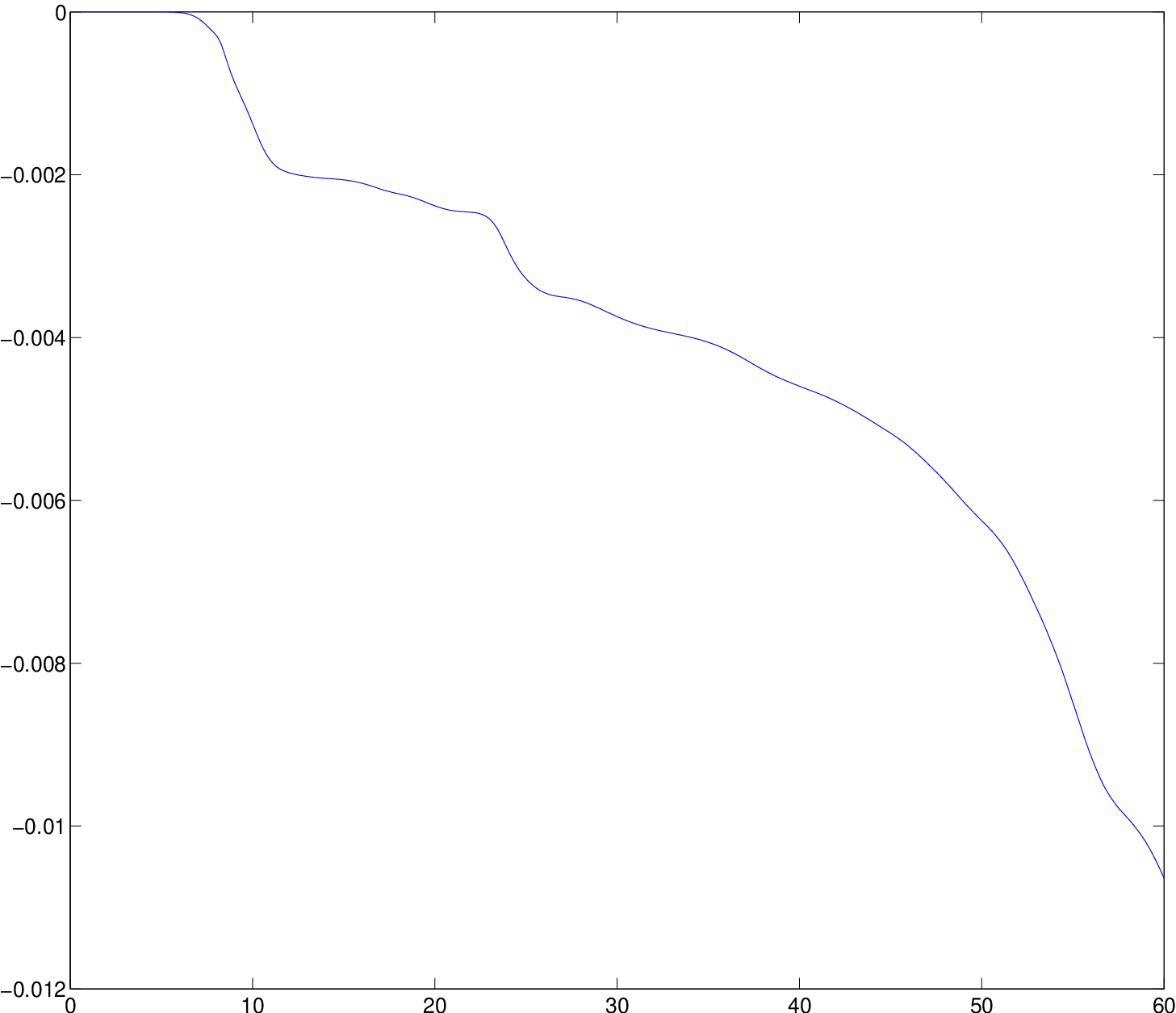
We wish to check now that there is no artificial damping due to the numerical scheme; in other words, that in the second stage the decrease of the $l^{2}-$ norm of the solution has the right value. Using the notations of Section 3.2, this right value is given by the equality:

||u^{n+1}||_{l^{2}}=e^{-2\nu_{1}\mathbf{\delta x}{kx}}||u^{n\#}||_{l^{2}}.

Going back to Equation (28), we can write it under the form (assuming no artificial boundary layer: $B_{j}=0$ )

u^{n+1}_{j}=\frac{1-a-ib}{1+a+ib}u^{n\#}_{\theta_{j}},

where we set $a=\frac{\delta x}{2k_{x}}\nu_{1,j}^{n}$ and $b=\frac{\delta x}{2k_{x}}\mu_{j}.$ Since the characteristic value of the coefficient $a$ is $10^{-4}$ (or smaller) and, in the worst case, the characteristic value of $\mu$ is in the order of $1,$ so that we can choose $\frac{\delta x}{2k_{x}}$ to have $b$ small, we see that

|\frac{1-a-ib}{1+a+ib}|^{2}=1-4a\frac{1}{1+b^{2}}+o(a^{2}),

which is very close to the right value $e^{-4a}=1-4a+o(a^{2}).$ The only damping may then come from the fact that $\sum\limits_{j}|u^{n\#}_{\theta_{j}}|^{2}$ may be significantly smaller than $\sum\limits_{j}|u^{n\#}_{j}|^{2},$ due to a large difference between $u^{n\#}_{j}$ and $u^{n\#}_{j-1}.$ To check this numerically, we test the case $\nu=0:$ Figure 10 shows that even in a difficult case with a large $\alpha=1.5,$ the global energy $||u^{n}||^{2}_{l^{2}}$ is conserved.

3.3.4 Two-ray model

We have also performed computations for the two-ray model which is described above at Section 3.1.4 using two functions $u^{1}$ and $u^{2}$ ; an illustration is given by Figure 12. The interaction between the rays is only given by the nonlinear term $f(w)$ with $w^{2}=|u^{1}|^{2}+|u^{2}|^{2}$ as above. To analyse its exact influence, one can compare the result given by the previous model with the two-ray interaction and the result given by a simple superposition of two independant rays (obtained with the one-ray model). One may see then that the energy becomes larger with the two-ray interaction: on the case of Figure 12 for instance, $Max(|u^{1}|^{2}+|u^{2}|^{2})=12.3$ instead of $10.6$ if the rays do not interact.

4 Extension to a Time-Dependent Interaction Model

We now address a model where a tilted paraxial equation is coupled with a hydrodynamic model in order to study filamentation. Under the hypothesis of a small incidence angle, this model has been extensively used by physicists for a long time and it is also addressed in [4],[3],[10] for example and the references therein (for a derivation of this model, see [18] for example).

4.1 The Model and the Numerical Method

Modeling of the plasma.

By taking the critical density (depending only on the laser wave length) as a reference density, one defines a non-dimension electron density $N=N(t,\mathbf{x})$ ; so the plasma may be characterized only by this quantity, the plasma velocity $\mathbf{U}=\mathbf{U}(t,\mathbf{x})$ and the electron density $T_{e}(t,\mathbf{x})$ .

Then, the simplest model is the following one. The pressure $P=P(N,T_{e})$ is assumed to be a smooth function of the density $N$ and of the electron temperature $T_{e}$ (which is assumed to be a very smooth fixed function of the position $\mathbf{x}$ ), for example $P(N,T_{e})$ may be the sum of two terms equal to $N^{3}$ and $NT_{e}$ up to multiplicative constants. Then one considers the following barotropic Euler system:

	$\displaystyle\frac{\partial}{\partial t}N+\nabla(N\mathbf{U})$	$\displaystyle=$	$\displaystyle 0,$		(33)
	$\displaystyle\frac{\partial}{\partial t}(N\mathbf{U})+\nabla(N\mathbf{UU})+\nabla(P(N,T_{e}))$	$\displaystyle=$	$\displaystyle-N\gamma_{p}\nabla\|\Psi\|^{2}.$		(34)

The term $\gamma_{p}\nabla|\Psi|^{2}$ corresponds to a ponderomotive force due to a laser pressure (the coefficient $\gamma_{p}$ is a constant depending only on the ion species).

Modeling of the laser beam.

The laser field $\Psi=\Psi(t,\mathbf{x})$ is a solution to the following frequency wave equation (which is of Schrödinger type):

2i\frac{1}{c}\frac{\partial}{\partial t}\Psi+\frac{1}{k_{0}}\Delta\Psi+k_{0}(1-N)\Psi+i\nu^{\diamond}\Psi=0,

(35)

where the real coefficient $\nu^{\diamond}$ is related to the absorption of the laser intensity by the plasma and $c$ the light speed.

Assume that the mean value of the plasma density is quite constant and denoted $N_{m}$ , so we set:

N(\mathbf{x})=N_{m}+\delta N(\mathbf{x}),

where $\delta N$ is small with respect to $1.$ Then one can make the paraxial approximation ; that is to say the laser beam is now characterized by the space and time envelope of the electric field $\mathcal{U}=\mathcal{U}(t,\mathbf{x})$ and we set:

\Psi(t,\mathbf{x})=\mathcal{U}(t,\mathbf{x})e^{ik_{0}\mathbf{K}.\mathbf{x}},\qquad{\rm where}\;\mathbf{K}=\sqrt{1-N_{m}}\mathbf{k}.

Therefore, if one sets $\epsilon=\frac{1}{k_{0}\sqrt{1-N_{m}}},$ by the same procedure as mentioned in the introduction, one checks that $\mathcal{U}$ satisfies:

\sqrt{1-N_{m}}(i\mathbf{k.}\nabla\mathcal{U}+\frac{\epsilon}{2}\Delta_{\bot}^{k}\mathcal{U})+i\frac{\nu^{\diamond}}{2}\mathcal{U}-\frac{k_{0}\delta N}{2}\mathcal{U}+i\frac{1}{c}\frac{\partial\mathcal{U}}{\partial t}=0.

(36)

It is necessary to supplement equation (36) with the same boundary condition as in the model of section 1 (and with an initial condition).

Numerical method.

We consider a mesh of finite difference type as above. The numerical treatment of the barotropic Euler system (33)(34) is a classical one, we have chosen a Lagrange-Euler method, see [3] for details. To deal with (36), according to the large value of the speed of light, one must perform a time inplicit discretization. So at each time step, one solves firstly the Euler system with a ponderomotive force evaluated with the previous value of $|\mathcal{U}|^{2}.$ Secondly, using the obtained values of $N$ and of $\delta N,$ one has to solve (36) ; if $u^{ini}$ and $u$ denote the values of the field $\mathcal{U}$ at the beginning and the end of time step, one searches $u$ solution to:

i\mathbf{k.}\nabla u+i\nu u+\frac{\epsilon}{2}(\Delta_{\bot}^{k}u)-\mu u=\frac{i}{c\sqrt{1-N_{m}}}\frac{u^{ini}}{\delta t},

(37)

where we have set:

\mu=\frac{k_{0}\delta N}{2\sqrt{1-N_{m}}},\qquad\nu=\frac{1}{c\sqrt{1-N_{m}}}\frac{1}{\delta t}+\frac{1}{2\sqrt{1-N_{m}}}\nu^{\diamond}.

That is exactly the equation studied in section 3, but a right hand side term has been added. So the numerical method is the same as described above ; the only modification is the adding of the right hand side term in the transport stage. Notice that the index of refraction $(1-N)$ is equal to $(1-2\epsilon\mu)(1-N_{m}).$

>From a practical point of view, the numerical method for (36) has been implemented in a parallel way in the HERA plateform for plasma hydrodynamics in 2D and in 3D; the parallel solver and the domain decomposition techniques are the same as the ones detailed in [3].

4.2 Numerical Results

Recall that from a practical point of view, in the transverse profile of a laser beam, one distinguishes a lot of small hot spots, called speckles, whose intensity is very large compared to the mean intensity of the beam. The shape of each individual speckle is a Gaussian function whose width is about a few micrometers. We present here the results of a 2D numerical simulation. One addresses a simulation box which is 600 $\mu$ m long and 300 $\mu$ m wide, the laser propagates with an incidence angle of $19^{0}.$ The incoming boundary condition $\alpha=\alpha(y)$ is independent of time and mimics a laser beam whose width is equal to $40\mu m$ with five speckles ; each speckle is modeled by a centered Gaussian function $h$ and is characterized by a random phase $\zeta_{k}$ , that is to say $\alpha(y)=\Sigma_{k=1}^{5}a_{k}h(y-y_{k})e^{i\zeta_{k}},$ where the $\alpha_{k}$ are random and the $a_{k}$ are close to each other. The plasma has an initial density equal to $N_{m}=0.15$ and the temperature is equal to $35.\ 10^{6}$ Kelvin. The mesh consists of 4 millions of cells and the time step is in the order of 0.1 picosecond (it is determined at each time step by the Courant-Friedrichs-Levy condition related to the sound speed of the plasma). The initial value of the laser intensity is zero, the plasma is progressively grabed by the ponderomotive force and on Figure 13, we have plotted the laser intensity at different times. At the first snapshot (at time $2.6$ ps), the plasma is not grabed enough, so the value of $\mu$ is small; the autofocusing effect is very low but not negligible: instead of five different speckles at the incoming boundary one notices only four speckels at the rear side (one of the four has a larger intensity) and a little spreading of the beam may be observed. At the second snapshot, the position of the four speckles has changed and the plasma is more grabed - since the energy density is larger in one speckle. On the two last snapshots, we may check that the spreading of the beam at the rear side of the simulation box becomes larger when the time increases. Moreover the configuration is not stationary, this situation is characteristic of the so-called filamentation instability.

Conclusion

A mathematical analysis has lead to an analytical form of the solution of the tilted paraxial equation in the simple case where the refraction index and the absorption coefficients are constant. Afterwards, we proposed a numerical method for solving the initial problem which uses the previous analytical form. The scheme has the property to yield a classical scheme when incidence angle becomes zero and the equation reduces to the classical paraxial one. The numerical method is illustrated by some results on toy problems. We have also given extensions of this model, which have enlarged the capability of our plateform HERA for laser propagation in a plasma (see [3] and [14] for examples of simulations performed with HERA). This numerical method may be also extended in the case where the unit vector $\mathbf{K}$ depends slowly on the one-dimension spatial variable $\mathbf{x}.\mathbf{n}$ , for instance if one has to deal with an equation of the following type

i\mathbf{K}.\nabla u+i\frac{1}{2}(\nabla.\mathbf{K})u+\frac{1}{2k_{0}}\Delta^{\mathbf{k}}_{\bot}u-\mu u+i\nu u=0,\quad{\rm on}\;{\cal D}.

The paraxial equation in a tilted frame may be also considered in a first region where the plasma density is slowly varying with respect to the spatial variable and coupled with another model in a neighbor region where the plasma density is strongly varying: in that region the laser is no more characterized by the time-space envelope of the fast oscillating electric field but by the wave equation (35) (see [6], for results obtained in HERA with this model). For simulating such a physical tilted beam, a classical paraxial model without accounting for the incidence angle would lead to search a the solution which would be highly oscillating with respect to the space variable and therefore to increase dramatically the mesh size to get accurate results.

References

[1] A. Arnold, Numerically Absorbing Boundary Conditions for Quantum Evolution Equations, VLSI Design 6 No. 1-4 p. 313-319, (1998).
[2] J.P. Bérenger, A Perfecly Matched Layer, J. Comp. Physics 114, p. 185-200 (1994).
[3] Ph. Ballereau, M. Casanova, F. Duboc et al., Simulation of the Paraxial Laser Propagation coupled with Hydrodynamics in 3D Geometry, J. Scientific Comp. 33, p.1-24, (2007).
[4] R.L. Berger, B.F. Lasinski et al., Theory and three-dimensional Simulation of Light Filamentation, Phys. Fluids B, 5, p. 2243-2258 (1993).
[5] M. Doumic, Boundary value problem for an oblique paraxial model, to appear.
[6] S. Desroziers, F. Nataf, R. Sentis, Simulation of Laser Propagation in a plasma with a Frequency Wave Equation, J. Comp. Physics, 227, p. 2610-2625 (2008).
[7] L. Di Menza, Transparent and Absorbing Boundary Conditions for Schrödinger Equations, Num. Funct. Anal. Optimization, 18, p 759 (1997).
[8] J. D. Lindl et al., The physics basis for ignition using indirect-drive target (§III), Phys. Plasmas, 11, pp. 339-491 (2004)
[9] M. Doumic, Etude asymptotique et simulation numérique de la propagation laser en milieu inhomogène, Ph. D. Dissertation, University Paris VII, (2005).
[10] M. R. Dorr, Garaizar F. X., Hittinger J. A., Simuation of laser-Plasma filamentation, J. Comp. Phys., 177, p.233-263 (2002).
[11] H. Dym, H.P. McKean, Fourier Series and Integrals, Academic Press, (1972).
[12] M. Ehrhardt, A. Arnold, Discrete Transparent Boundary Conditions for Schrödinger Equations, Riv. Mat. Univ. Parma, 6, p. 57 (2001).
[13] M.D. Feit, J.A. Fleck, Beam non paraxiality, J. Opt.Soc.Am. B, 5 , p633-640 (1988).
[14] P. Loiseau et al., Laser beam smoothing induced by simulated Brillouin scattering, Phys. Rev. Letters, 97, p.205001 (2006).
[15] R. Hadley, Transparent Boundary Condition for the Beam Propagation Method, IEEE, J. Quantum Electronics, 28, p.363 (1992).
[16] D. Lee, A. D. Pierce, E.-S. Shang, Parabolic Equation Development in the twentieth century, J. Comput. Acoust., 8 (2000), p.527-637.
[17] R. J. LeVeque, Numerical Methods for Conservation Laws, Birkhauser-Verlag, Basel, 1990.
[18] R. Sentis, Mathematical models for laser-plasma interaction, ESAIM-Mathematical Modelling and Numerical Analysis, 39, p. 275–318 (2005).
[19] H.A. Rose, Laser beam deflection, Phys. Plasmas, 3, p. 1709-1727 (1996).
[20] V.T. Tikhonchuk, A.A. Zozulya, Structure of Light beams in self-pumped four wave mixing geometries, Prog.Quant. Electr., 15, p.231 (1992).
[21] F. Walraet, G. Riazuelo, G. Bonnaud, Propagation in a plasma of a smooth Laser Beam, Phys. Plamas, 10, p. 811-919 (2003).

Simulation of Laser Beam Propagation With a Paraxial Model in a Tilted Frame

Abstract

1 Introduction

2 Analysis of the Tilted Paraxial Equation

2.1 Energy Estimate

Proposition 1

2.2 Analytical Form of the Solution in the Case νt\nu_{t} Constant

Proposition 2

Corollary 1

2.3 Remark on the Problem on the Quadrant

Proposition 3

3 Numerical Scheme

3.1 Description of the Scheme

3.1.1 Initialization

3.1.2 First stage: Fourier transform

3.1.3 Second stage: finite difference scheme

3.1.4 Numerical method for two-ray model

3.2 Properties of the scheme

3.2.1 Stability

Proposition 4

3.2.2 Comparison with the classical Schrödinger equation

Proposition 5

3.3 Numerical results

3.3.1 Convergence of the scheme

3.3.2 Variation of several parameters

3.3.3 Remark on artificial damping

3.3.4 Two-ray model

4 Extension to a Time-Dependent Interaction Model

4.1 The Model and the Numerical Method

4.2 Numerical Results

Conclusion

References

2.2 Analytical Form of the Solution in the Case $\nu_{t}$ Constant