Measuring the ”non-stopping timeness” of ends of previsible sets

Ju-Yi Yen^(1),(2) Address: (1) Vanderbilt University, Nashville, Tennessee 37240, USA Email address: ju-yi.yen@vanderbilt.edu Address: (2) Institute of Mathematics, Academia Sinica, Taipei, Taiwan Current address: and Marc Yor^(3),(4) Address: (3) Laboratoire de Probabilités et Modèles Aléatoires, Université Pierre et Marie Curie, Case Courrier 188, 4, Place Jussieu, 75252 Paris, Cedex 05, France Address: (4) Institut Universitaire de France Email address:

Date: October 3, 2008

Abstract.

In this paper, we propose several ”measurements” of the ”non-stopping timeness” of ends $\mathcal{G}$ of previsible sets, such that $\mathcal{G}$ avoids stopping times, in an ambiant filtration. We then study several explicit examples, involving last passage times of some remarkable martingales.

Key words and phrases:

Azéma supermartingale, last passage times

1. Introduction: About ends of previsible sets

In this paper, we are interested in random times $\mathcal{G}$ defined on a filtered probability space $(\Omega,\mathcal{F},(\mathcal{F}_{t}),P)$ as ends of $(\mathcal{F}_{t})$ previsible sets $\Gamma$ , that is:

\mathcal{G}\equiv\mathcal{G}_{\Gamma}=\sup\{t:\ (t,\omega)\in\Gamma\}

(1)

For simplicity, we shall make the following assumptions:

(C):: All $((\mathcal{F}_{t}),P)$ martingales are continuous;
(A):: For any $(\mathcal{F}_{t})$ stopping time $T$ , $P(\mathcal{G}=T)=0$ .

[(C) stands for ”continuous”, and (A) for ”avoiding”].
To such a random time, one associates the Azéma supermartingale:

Z_{t}^{\mathcal{G}}=P(\mathcal{G}>t|\mathcal{F}_{t}),

(2)

which, under (CA), admits a continuous version.

In a number of questions, it is very interesting to consider the smallest filtration $(\mathcal{F}_{t}^{\prime})_{t\geq 0}$ , which contains $(\mathcal{F}_{t})$ , and makes $\mathcal{G}$ a stopping time; this filtration is usually denoted $(\mathcal{F}_{t}^{\mathcal{G}})_{t\geq 0}$ . One of the interests of $(Z_{t}^{\mathcal{G}})$ is that it allows to write any $(\mathcal{F}_{t})$ martingale as a semimartingale in $(\mathcal{F}_{t}^{\mathcal{G}})_{t\geq 0}$ ; see e.g. [2, 3, 8, 9], for both general formulae and many examples.

Recently, it has been understood that Black-Scholes like formulae are closely related with certain such $\mathcal{G}$ ’s, thus throwing a new light on a cornerstone of Mathematical Finance, see, e.g. [6, 7]. In the present paper, with (A) as our essential hypothesis, we would like to measure ”how much $\mathcal{G}$ differs from a $(\mathcal{F}_{t})$ stopping time”. The remainder of this paper consists in two sections: - In Section 2, we propose several criterions to measure the NST ( $\equiv$ Non Stopping Timeness) of $\mathcal{G}$ ’s which satisfy (CA); it is not surprising that we get interested in the function:

m_{\mathcal{G}}(t)=E\left[\left(1_{(\mathcal{G}\geq t)}-P(\mathcal{G}\geq t|\mathcal{F}_{t})\right)^{2}\right].

- In Section 3, we compute explicitly this function $m_{\mathcal{G}}$ for various examples, where $\mathcal{G}$ is the last passage time at a level of a martingale which converges to 0, as $t\rightarrow\infty$ .

2. Several possible ”NST” criterions

2.1. A fundamental function: $m_{\mathcal{G}}(t)$

Let us consider several possible criterions: first of all, if $\mathcal{G}$ were a $(\mathcal{F}_{t})$ stopping time, then the process $1_{(\mathcal{G}\geq t)}$ would be identically equal to $Z_{t}^{\mathcal{G}}\equiv P(\mathcal{G}\geq t|\mathcal{F}_{t})$ . Thus, the function $(m_{\mathcal{G}}(t),\ t\geq 0)$ tells us about the NST of $\mathcal{G}$ . Next, a simple but useful remark is that:

m_{\mathcal{G}}(t)=E\left[Z_{t}^{\mathcal{G}}\left(1-Z_{t}^{\mathcal{G}}\right)\right].

(3)

2.2. Definition of $m_{\mathcal{G}}^{*}$ , $m_{\mathcal{G}}^{}$ , and $\widetilde{m}_{\mathcal{G}}$ and proof that $m_{\mathcal{G}}^{}=1/4=\widetilde{m}_{\mathcal{G}}$

Instead of considering the ”full”function $(m_{\mathcal{G}}(t),\ t\geq 0)$ , we may consider only:

m_{\mathcal{G}}^{*}=\underset{t\geq 0}{\sup}\ m_{\mathcal{G}}(t)

(4)

as a ”global” measurement of the NST of $\mathcal{G}$ .

Here are two other, a priori natural, measurements of the NST of $\mathcal{G}$ :

m_{\mathcal{G}}^{**}=E\left[\underset{t\geq 0}{\sup}\left(Z_{t}^{\mathcal{G}}\left(1-Z_{t}^{\mathcal{G}}\right)\right)\right]

(5)

and

\widetilde{m}_{\mathcal{G}}=\underset{T\geq 0}{\sup}\ E\left[Z_{T}^{\mathcal{G}}\left(1-Z_{T}^{\mathcal{G}}\right)\right]

(6)

where $T$ runs over all $(\mathcal{F}_{t})$ stopping times.

However, we cannot expect to learn very much from $m_{\mathcal{G}}^{**}$ and $\widetilde{m}_{\mathcal{G}}$ , since it is easily shown that

m_{\mathcal{G}}^{**}=1/4=\widetilde{m}_{\mathcal{G}}.

(7)

Proof.

(i)

The fact that $m^{**}_{\mathcal{G}}=1/4$ follows immediately from:
$\underset{x\in[0,1]}{\sup}\ (x(1-x))=1/4$ , and the fact that, a.s., the range of the process $(Z_{t}^{\mathcal{G}},t\geq 0)$ is $[0,1]$ since $Z_{0}^{\mathcal{G}}=1$ , $Z_{\infty}^{\mathcal{G}}=0$ , and $(Z_{t}^{\mathcal{G}},t\geq 0)$ is continuous.
(ii)

Let us consider $T_{a}=\inf\{t:Z_{t}^{\mathcal{G}}=a\}$ , for $0<a<1$ . Then:
$Z_{t}^{\mathcal{G}}(1-Z_{t}^{\mathcal{G}})\mid_{t=T_{a}}=a(1-a)$ ; hence,
$\underset{a\in]0,1[}{\sup}\left[Z_{T_{a}}^{\mathcal{G}}\left(1-Z_{T_{a}}^{\mathcal{G}}\right)\right]=\underset{a\in]0,1[}{\sup}\left(a(1-a)\right)=1/4.$

∎

2.3. The optional stopping time discrepancy $\mu_{\mathcal{G}}$

Let us not forget either the nice characterization [4], of stopping times, among random times, as the times $\tau$ such that for every bounded martingale $(M_{t})_{t\geq 0}$ one has

M_{\tau}=E\left[M_{\infty}|\mathcal{F}_{\tau}\right]

where, here under our hypothesis (C), we may define $\mathcal{F}_{\tau}=\sigma\{H_{\tau};\ H\ \mbox{previsible}\}$ . Thus, as a 4th possible measurement of the NST of $\mathcal{G}$ , we may take:

\mu_{\mathcal{G}}=\underset{\underset{E(M_{\infty}^{2})\leq 1}{M_{\infty}\in L^{2}(\mathcal{F}_{\infty})}}{\sup}E\left[\left(M_{\mathcal{G}}-E\left[M_{\infty}|\mathcal{F}_{\mathcal{G}}\right]\right)^{2}\right].

(8)

2.4. Distance from stopping times

We introduce:

\nu_{\mathcal{G}}=\underset{T\geq 0}{\inf}E\left[|\mathcal{G}-T|\right]

where $T$ runs over all $(\mathcal{F}_{t})$ stopping times. However, this quantity may be infinite as $\mathcal{G}$ may have infinite expectation. A more adequate distance may be:

\nu_{\mathcal{G}}^{\prime}=\underset{T\geq 0}{\inf}\left(E\left[\frac{|\mathcal{G}-T|}{1+|\mathcal{G}-T|}\right]\right)

We note that this distance was precisely computed by du Toit-Peskir-Shiryaev in the example they consider [1].

It would be nice to be able to estimate $\mu_{\mathcal{G}}$ and/or $\nu_{\mathcal{G}}$ , $\nu_{\mathcal{G}}^{\prime}$ in terms of the function $m_{\mathcal{G}}(t)$ , but we have not been able to obtain any result in this direction. We shall now concentrate uniquely on the study of $(m_{\mathcal{G}}(t),\ t\geq 0)$ .

3. A study of several interesting examples of functions $m_{\mathcal{G}}(t)$

3.1. Some general formulae

We shall compute $(m_{\mathcal{G}}(t),\ t\geq 0)$ in some particular cases where:

\mathcal{G}=\mathcal{G}_{K}=\sup\{t\geq 0:M_{t}=K\},\ K\leq 1,

with $M_{0}=1$ , $M_{t}\geq 0$ , a continuous local martingale such that $M_{t}\underset{t\rightarrow\infty}{\longrightarrow}0$ , we recall that (see, e.g. [2, 8]):

Z_{t}=P(\mathcal{G}_{K}\geq t|\mathcal{F}_{t})=1\wedge\left(\frac{M_{t}}{K}\right)

thus

m(t)=E\left[Z_{t}\left(1-Z_{t}\right)\right]=\frac{1}{K^{2}}E\left[M_{t}\left(K-M_{t}\right)^{+}\right]

(9)

3.2. The particular case $M_{t}=\mathcal{E}_{t}=\exp(B_{t}-t/2)$ , with $(B_{t})$ a standard Brownian motion, and $\mathcal{G}_{K}=\sup\{t:\mathcal{E}_{t}=K\}$ , $(K\leq 1)$

From formula (9), we deduce:

$\displaystyle m_{K}(t)$	$\displaystyle=$	$\displaystyle\frac{1}{K^{2}}E\left[\mathcal{E}_{t}\left(K-\mathcal{E}_{t}\right)^{+}\right]$
	$\displaystyle=$	$\displaystyle\frac{1}{K^{2}}E\left[\left(K-\exp\left(B_{t}+\frac{t}{2}\right)\right)^{+}\right]\ \ \mbox{(by Cameron-Martin)}$
	$\displaystyle=$	$\displaystyle\frac{1}{K^{2}}\left\{KP\left(\exp\left(B_{t}+\frac{t}{2}\right)<K\right)\right.$
		$\displaystyle\ \ \ \left.-E\left[1_{\left(\exp\left(B_{t}+\frac{t}{2}\right)<K\right)}\exp\left(B_{t}+\frac{t}{2}\right)\right]\right\}$
$\displaystyle(K=e^{l})$	$\displaystyle=$	$\displaystyle e^{-l}P\left(B_{t}+\frac{t}{2}<l\right)-e^{t}e^{-2l}P\left(B_{t}+\frac{3t}{2}<l\right)$
	$\displaystyle=$	$\displaystyle P\left(B_{1}<-\frac{3\sqrt{t}}{2}+\frac{l}{\sqrt{t}}\right)\left(e^{-l}-e^{t-2l}\right)$
		$\displaystyle\ \ \ \ +e^{-l}P\left(-\frac{3\sqrt{t}}{2}+\frac{l}{\sqrt{t}}<B_{1}<-\frac{\sqrt{t}}{2}+\frac{l}{\sqrt{t}}\right).$

Particularizing again, for $M_{t}=\mathcal{E}_{t}=\exp(B_{t}-t/2)$ , and $K=1$ , then

	$\displaystyle m(t)$	$\displaystyle=$	$\displaystyle E\left[\mathcal{E}_{t}\left(1-\mathcal{E}_{t}\right)^{+}\right]$		(10)
		$\displaystyle=$	$\displaystyle P\left(B_{1}<-\frac{3\sqrt{t}}{2}\right)\left(1-e^{t}\right)+P\left(-\frac{3\sqrt{t}}{2}<B_{1}<-\frac{\sqrt{t}}{2}\right).$		(10)

Figure 1 presents the graphs of $m_{K}(t)$ for some $K$ ’s.

Refer to caption — Figure 1. Graphs of $m_{K}(t)$ , for $K=0.1,0.2,...1.$

Comments: It seems that $m_{K}^{*}=\underset{t\geq 0}{\sup}\ (m_{K}(t))$ increases with $K$ , at least for $K\leq 1$ . Can this be proven? If so, it indicates that, as $K$ varies, the $\mathcal{G}_{K}$ ’s are increasingly further from stopping times.

3.3. The case $\mathcal{G}=\mathcal{G}_{T_{a}}=\sup\{t<T_{a}:B_{t}=0\}$

From line 4 of Table $(1\alpha)$ of Progressive Enlargements, p.32 of [8], we obtain:

Z_{t}=1-\frac{1}{a}B^{+}_{t\wedge T_{a}}

Thus, we obtain:

$\displaystyle m_{\mathcal{G}}(t)$	$\displaystyle=$	$\displaystyle E\left[\left(\frac{1}{a}B_{t\wedge T_{a}}^{+}\right)\left(1-\frac{1}{a}B_{t\wedge T_{a}}^{+}\right)\right]$
	$\displaystyle=$	$\displaystyle\frac{1}{a^{2}}E\left[1_{(t<T_{a})}1_{(B_{t}>0)}B_{t}(a-B_{t})\right]$
	$\displaystyle=$	$\displaystyle\frac{1}{a^{2}}E\left[1_{(S_{t}<a)}1_{(B_{t}>0)}B_{t}(a-B_{t})\right]$
	$\displaystyle=$	$\displaystyle\frac{1}{a^{2}}E\left[\left(S_{1}<\frac{a}{\sqrt{t}}\right)1_{(B_{1}>0)}tB_{1}\left(\frac{a}{\sqrt{t}}-B_{1}\right)\right]$
	$\displaystyle=$	$\displaystyle\frac{1}{x^{2}}\varphi(x),\ \ \mbox{where: $x=\frac{a}{\sqrt{t}}$ and:}$
$\displaystyle\varphi(x)$	$\displaystyle=$	$\displaystyle E\left[1_{(S_{1}<x)}1_{(B_{1}>0)}B_{1}(x-B_{1})\right]$	(11)

Now, it remains to compute the function $\varphi$ . We note that

\varphi(x)=E\left[B_{1}^{+}(x-B_{1})^{+}\right]-E\left[1_{(S_{1}>x)}B_{1}^{+}(x-B_{1})^{+}\right].

We shall take advantage of the very useful formula:

P(S_{1}>x|B_{1}=a)=\exp(-2x(x-a)),\ x\geq a>0.

(This formula is easily seen to be equivalent to the well-known expression of the joint density of $(S_{1},B_{1})$ ; see, e.g., [5], p.425.) Thus, we find:

	$\displaystyle\varphi(x)$	$\displaystyle=$	$\displaystyle\frac{1}{\sqrt{2\pi}}\int_{0}^{x}dy\ y(x-y)\left(\exp\left(-\frac{y^{2}}{2}\right)-\exp\left(-\frac{1}{2}(2x-y)^{2}\right)\right)$
		$\displaystyle\equiv$	$\displaystyle\frac{x^{3}}{\sqrt{2\pi}}\int_{0}^{1}du\ u(1-u)\left(\exp\left(-\frac{x^{2}u^{2}}{2}\right)-\exp\left(-\frac{x^{2}}{2}(2-u)^{2}\right)\right)$

Thus:

\frac{\varphi(x)}{x^{2}}=\frac{x}{\sqrt{2\pi}}\int_{0}^{1}du\ u(1-u)\left(\exp\left(-\frac{x^{2}u^{2}}{2}\right)-\exp\left(-\frac{x^{2}}{2}(2-u)^{2}\right)\right).

3.4. The case $\mathcal{G}=L_{a}=\sup\{u:R_{u}=a\}$

From line 6 of Table $(1\alpha)$ of Progressive Enlargements, p.32 of [8], we obtain:

Z_{t}=1\wedge\left(\frac{a}{R_{t}}\right)^{2\mu}.

Here, $(R_{u})$ is $BES_{0}(d),\ d=2(\mu+1)$ . For that second example, we get:

$\displaystyle m_{\mathcal{G}}(t)$	$\displaystyle=$	$\displaystyle E\left[\left(1\wedge\left(\frac{a}{R_{t}}\right)^{2\mu}\right)\left(1-1\wedge\left(\frac{a}{R_{t}}\right)^{2\mu}\right)\right]$
	$\displaystyle=$	$\displaystyle E\left[1\left(\frac{a}{\sqrt{t}R_{1}}<1\right)\left(\frac{a}{\sqrt{t}R_{1}}\right)^{2\mu}\left(1-\left(\frac{a}{\sqrt{t}R_{1}}\right)^{2\mu}\right)\right]$
	$\displaystyle=$	$\displaystyle\varphi_{\mu}\left(\frac{a^{2}}{2t}\right)$

where using the fact that $R^{2}_{1}\stackrel{{\scriptstyle\rm{(law)}}}{{=}}2\gamma_{d/2}$ , we get (recall: $\frac{d}{2}=\mu+1$ ):

\varphi_{\mu}(z)=\frac{1}{\Gamma(\mu+1)}\left\{z^{\mu}e^{-z}-z^{2\mu}\int_{z}^{\infty}\frac{du}{u^{\mu}}e^{-u}\right\}.

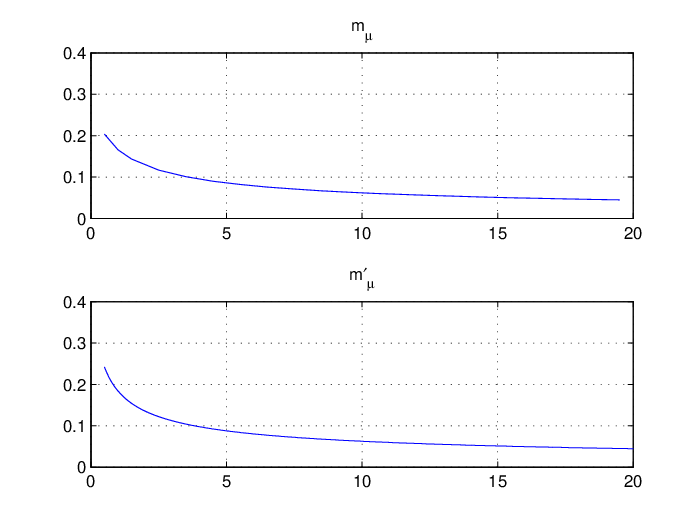
Figure 2 presents the graphs of $\varphi_{\mu}$ for $\mu=1/2,1,3/2,5/2,7/2,9/2,11/2$ and $13/2$ . We also approximate $z_{\mu}$ , the unique $>0$ real which achieves the max of $\varphi_{\mu}$ . This will give us the value $m_{\mu}\stackrel{{\scriptstyle\rm{def}}}{{=}}m_{\mathcal{G}}^{*}$ , for these $\mathcal{G}\equiv\mathcal{L}_{a}$ (note that, for a given $\mu$ , the value does not depend on $a$ ; this is because of the scaling property).

It is not difficult to show that: $z_{\mu}$ is the unique solution of

(E_{\mu}):\ \ \frac{1}{2z}=\int_{0}^{\infty}\frac{dh}{(1+h)^{\mu}}e^{-hz}

and also

m_{\mu}=\frac{1}{\Gamma(\mu+1)}e^{-z_{\mu}}\frac{(z_{\mu})^{\mu}}{2}.

Note that

m_{\mu}\leq m_{\mu}^{\prime}\stackrel{{\scriptstyle\rm{def}}}{{=}}\frac{1}{\Gamma(\mu+1)}\ \underset{z\geq 0}{\sup}\ \left(e^{-z}\frac{z^{\mu}}{2}\right).

Figure 3 presents the graphs of $m_{\mu}$ and $m_{\mu}^{\prime}$ .

References

[1] du Toit, J., Peskir, G. ,& Shiryaev, A. N. Predicting the last zero of Brownian motion with drift, Stochastics, 80: 229-245, 2008.
[2] Jeulin, T. Semi-martingales et grossissements d’une filtration, LNM 833, Springer, Berlin, 1980.
[3] Jeulin, T. & Yor, M. Eds. Grossissements de filtrations: exemples et applications, LNM 1118, Springer-Verlag, 1985.
[4] Knight, F. & Maisonneuve, B. A characterization of stopping times, The Annals of Probability, Vol. 22, No. 3 (July, 1994), pp. 1600-1606.
[5] Karatzas, I. & Shreve, M. Brownian Motion and Stochastic Calculus, 2nd ed. Springer, Berlin (1991).
[6] Madan, D., Roynette, R., & Yor, M. Option prices as probabilities, Finance Research Letters 5, 79-87 (2008), doi:10.1016/j.frl.2008.02.002
[7] Madan, D., Roynette, R., & Yor, M. Unifying Black-Scholes type formulae which involve last passage times up to finite horizon. To appear in Asia-Pacific Financial Markets (2008).
[8] Mansuy, R. & Yor, M. Random times and enlargements of filtrations in a Brownian setting, LNM 1873, Springer, Berlin, 2006.
[9] Nikeghbali, A. & Yor, M. Doob’s maximal identity, multiplicative decomposition and enlargements of filtrations, Ill. Journal of Maths., 50:791-814, 2006.

Measuring the ”non-stopping timeness” of ends of previsible sets

Abstract.

Key words and phrases:

1. Introduction: About ends of previsible sets

2. Several possible ”NST” criterions

2.1. A fundamental function: m𝒢​(t)m_{\mathcal{G}}(t)

2.2. Definition of m𝒢∗m_{\mathcal{G}}^{*}, m𝒢∗⁣∗m_{\mathcal{G}}^{**}, and m~𝒢\widetilde{m}_{\mathcal{G}} and proof that m𝒢∗⁣∗=1/4=m~𝒢m_{\mathcal{G}}^{**}=1/4=\widetilde{m}_{\mathcal{G}}

Proof.

2.3. The optional stopping time discrepancy μ𝒢\mu_{\mathcal{G}}

2.4. Distance from stopping times

3. A study of several interesting examples of functions m𝒢​(t)m_{\mathcal{G}}(t)

3.1. Some general formulae

3.2. The particular case Mt=ℰt=exp⁡(Bt−t/2)M_{t}=\mathcal{E}_{t}=\exp(B_{t}-t/2), with (Bt)(B_{t}) a standard Brownian motion, and 𝒢K=sup{t:ℰt=K}\mathcal{G}_{K}=\sup\{t:\mathcal{E}_{t}=K\}, (K≤1)(K\leq 1)

3.3. The case 𝒢=𝒢Ta=sup{t<Ta:Bt=0}\mathcal{G}=\mathcal{G}_{T_{a}}=\sup\{t<T_{a}:B_{t}=0\}

3.4. The case 𝒢=La=sup{u:Ru=a}\mathcal{G}=L_{a}=\sup\{u:R_{u}=a\}