In this section, we review the basic features of the two-site model (for more details see [30]). The particle content is divided into two sectors: composite and elementary. The elementary sector of the model is equal exactly to that of SM except for the Higgs field. The SM gauge fields ($SU(3)\otimes SU(2)_{L}\otimes U(1)_{Y}$) will be denoted in the following way,

$\displaystyle A_{\mu}\equiv\{G_{\mu},W_{\mu},B_{\mu}\}$

(1)

and fermion $SU(2)_{L}$ doublets by,

$\displaystyle\psi_{L}\equiv\{q_{Li}=(u_{Li},d_{Li}),l_{Li}=(\nu_{Li},e_{Li})\}$

(2)

and finally $SU(2)_{L}$ singlets as,

$\displaystyle\tilde{\psi}_{R}\equiv\{u_{Ri},d_{Ri},\nu_{Ri},e_{Ri}\}.$

(3)

The only renormalizable interactions are the gauge interactions.

$\displaystyle\mathcal{L}^{\small{\text{elementary}}}=-\frac{1}{4}F_{\mu\nu}^{2}+\bar{\psi}_{L}i\mathord{\not\mathrel{{\mathrel{D}}}}\psi_{L}+\bar{\tilde{\psi}}_{R}i\mathord{\not\mathrel{{\mathrel{D}}}}\tilde{\psi}_{R}.$

(4)

The composite boson sector (containing the SM Higgs and massive spin $1$ particles) has $SU(3)\otimes SU(2)_{L}\otimes SU(2)_{R}\otimes U(1)_{X}$ global symmetries, where we need the additional custodial $SU(2)_{R}$ to suppress new physics contribution to the $T$ parameter [7]. There are fifteen heavy vector mesons ($\rho_{\mu}$) that belong to adjoint representation of the $SU(3)\otimes SU(2)_{L}\otimes SU(2)_{R}\otimes U(1)_{X}$, and they can be decomposed into two sets: $\rho_{*}$, which are in the adjoint representation of the SM gauge group and their orthogonal combinations $\tilde{\rho}$

$$\rho^{*}_{\mu}=\{G_{\mu}^{*},W_{\mu}^{*},{\cal B}_{\mu}^{*}\}\,,\qquad\tilde{\rho}_{\mu}=\Big\{\tilde{W}^{\pm}_{\mu}\equiv\frac{\tilde{W}_{1}\mp i\,\tilde{W}_{2}}{\sqrt{2}},\tilde{\cal B}_{\mu}\Big\}\,.$$

(5)

We associate ${\cal B^{*}},{\cal\tilde{B}}$ with the generators $T_{{\cal B}^{*}}=Y_{\text{hypercharge}}=\frac{T^{3R}+\sqrt{2/3}T_{X}}{\sqrt{5/3}}$ and $T_{{\cal\tilde{B}}}=\frac{T^{3R}-\sqrt{2/3}T_{X}}{\sqrt{5/3}}$, where $T_{{\cal B}^{*}}$ is hypercharge generator in the SO(10) normalization. Higgs field belongs to the composite sector and is a real bidoublet under $SU(2)_{L}\otimes SU(2)_{R}$: $(H,\tilde{H})$.

Every SM fermion representation will be accompanied by a heavy composite Dirac fermion, so the composite sector will consist of $SU(2)_{L}$ doublets :

$\displaystyle\chi\equiv\left(Q_{i}=\{U_{i},D_{i}\},L_{i}=\{N_{i},E_{i}\}\right)$

(6)

and $SU(2)_{L}$ singlets:

$\displaystyle\tilde{\chi}=\left(\tilde{U}_{i},\tilde{D}_{i},\tilde{E}_{i},\tilde{N}_{i}\right)$

(7)

They are all singlets under $SU(2)_{R}$. The Dirac masses of the composite sector doublets and singlets are $m_{*},\tilde{m}_{*}$, respectively, which we assume to be the same (and generation-independent) for simplicity. $U(1)_{X}$ charges for fermions are chosen to reproduce the usual SM hypercharges.

The Lagrangian of the composite sector is

	$\displaystyle\mathcal{L}_{\small{\text{composite}}}=-\frac{1}{4}\rho_{\mu\nu}^{2}+\frac{M_{*}^{2}}{2}\rho_{\mu}^{2}+|D_{\mu}H|^{2}-V(H)+$
	$\displaystyle+\bar{\chi}(i\mathord{\not\mathrel{{\mathrel{D}}}}-m_{*})\chi+\bar{\tilde{\chi}}(i\mathord{\not\mathrel{{\mathrel{D}}}}-\tilde{m}_{*})\tilde{\chi}-\bar{\chi}(Y^{u}_{*}\tilde{H}\tilde{\chi}^{u}+Y^{d}_{*}H\tilde{\chi}^{d})+h.c.$		(8)

where $M_{*}$ is the mass of the composite sector vector boson (again, assumed to be the same for all gauge bosons for simplicity). One can see that Yukawa couplings explicitly break $SU(2)_{R}$ in composite sector (see Eq. (8)). But this breaking gives a small contribution to the $T$ parameter and is thus technically natural as mentioned in [30].⁴⁴ 4 Alternatively, we can add extra composite site fermions so that Yukawa interactions respect $SU(2)_{R}$. This corresponds to choosing $5D$ fermions in complete multiplets of $SU(2)_{R}$ in the $5D$ AdS models [7]. We will not pursue this option here.

The two sectors (composite and elementary) are connected to each other by the mixing terms

$${\cal L}_{\small{\text{mixing}}}=-M_{*}^{2}\,\frac{g_{el}}{g_{*}}\,A_{\mu}\rho_{\mu}^{*}+\frac{M_{*}^{2}}{2}\left(\frac{g_{el}}{g_{*}}A_{\mu}\right)^{2}+(\bar{\psi}_{L}\Delta\chi_{R}+\bar{\tilde{\psi}}_{R}\tilde{\Delta}\tilde{\chi}_{L}+{\rm h.c.}).$$

(9)

Due to the presence of the gauge boson mixing terms the following combination of the vector bosons will remain massless

$$\frac{g_{*}}{\sqrt{g_{el}^{2}+g_{*}^{2}}}\,A_{\mu}+\frac{g_{el}}{\sqrt{g_{el}^{2}+g_{*}^{2}}}\,\rho^{*}_{\mu}.$$

(10)

The original elementary and composite states will be re-written using the mass eigenstates as follows

	$\displaystyle\begin{pmatrix}A_{\mu}\\ \rho^{*}_{\mu}\end{pmatrix}$	$\displaystyle\rightarrow\begin{pmatrix}\cos\theta&-\sin\theta\\ \sin\theta&\cos\theta\end{pmatrix}\begin{pmatrix}A_{\mu}\\ \rho^{*}_{\mu}\end{pmatrix}\,,\quad$	$\displaystyle\tan\theta$	$\displaystyle=\frac{g_{el}}{g_{*}}\,,$		(11)
	$\displaystyle\begin{pmatrix}\psi_{L}\\ \chi_{L}\end{pmatrix}$	$\displaystyle\rightarrow\begin{pmatrix}\cos\varphi_{\psi_{L}}&-\sin\varphi_{\psi_{L}}\\ \sin\varphi_{\psi_{L}}&\cos\varphi_{\psi_{L}}\end{pmatrix}\begin{pmatrix}\psi_{L}\\ \chi_{L}\end{pmatrix}\,,\quad$	$\displaystyle\tan\varphi_{\psi_{L}}$	$\displaystyle=\frac{\Delta}{m_{*}}\,,$		(12)
	$\displaystyle\begin{pmatrix}\tilde{\psi}_{R}\\ \tilde{\chi}_{R}\end{pmatrix}$	$\displaystyle\rightarrow\begin{pmatrix}\cos\varphi_{\tilde{\psi}_{R}}&-\sin\varphi_{\tilde{\psi}_{R}}\\ \sin\varphi_{\tilde{\psi}_{R}}&\cos\varphi_{\tilde{\psi}_{R}}\end{pmatrix}\begin{pmatrix}\tilde{\psi}_{R}\\ \tilde{\chi}_{R}\end{pmatrix}\,,\quad$	$\displaystyle\tan\varphi_{\tilde{\psi}_{R}}$	$\displaystyle=\frac{\tilde{\Delta}}{\tilde{m}_{*}}\,.$		(13)

In the new, i.e., mass eigenstate basis, $(A_{\mu},\psi_{L},\tilde{\psi}_{R})$ are the SM fields, which are massless before EWSB, and $(\rho_{*}^{\mu},\chi_{L},\tilde{\chi}_{R})$ are the heavy mass eigenstates (i.e. the heavy partners of SM), again prior to EWSB. To shorten our notations we will denote

	$\displaystyle\theta\equiv\theta_{1},\theta_{2},\theta_{3},~~\varphi_{\psi_{L}}\equiv\varphi_{q_{Li}},\varphi_{l_{Li}},~~\varphi_{\tilde{\psi}_{R}}\equiv\varphi_{u_{Ri}},\varphi_{d_{Ri}},\varphi_{\nu_{Ri}},\varphi_{e_{Ri}}$
	$\displaystyle\sin\varphi_{u^{i}_{R}}\equiv s_{u},~~\sin\varphi_{d^{i}_{R}}\equiv s_{d},~~\sin\varphi_{q_{Li}}\equiv s_{q}.$		(14)

Substituting Eq. (11) (12) (13) in Eq. (8), we get the Lagrangian for the Yukawa interaction between quarks and Higgs field in mass eigenstates before EWSB (the same expression will be true for leptons too, one just has to substitute $L,E,N\Longleftrightarrow Q,D,U$)

	$\displaystyle{\cal L}_{Y}=$		$\displaystyle{\cal L}^{\text{SM-SM}}_{Y}+{\cal L}^{\text{SM-Heavy}}_{Y}+{\cal L}^{\text{Heavy-Heavy}}_{Y}$
	$\displaystyle=$		$\displaystyle-Y_{*u}\tilde{H}s_{q}s_{u}\bar{q}_{L}u_{R}-Y_{*d}{H}s_{q}s_{d}\bar{q}_{L}d_{R}$		(15)
			$\displaystyle-Y_{*u}\tilde{H}\left[c_{q}s_{u}\bar{Q}_{L}u_{R}+s_{q}c_{u}\bar{q}_{L}\tilde{U}_{R}\right]-Y_{*d}H\left[c_{q}s_{d}\bar{Q}_{L}d_{R}+s_{q}c_{d}\bar{q}_{L}\tilde{D}_{R}\right]$
			$\displaystyle-Y_{*u}\tilde{H}\left[c_{q}c_{u}\bar{Q}_{L}\tilde{U}_{R}+\bar{Q}_{R}\tilde{U}_{L}\right]-Y_{*d}{H}\left[c_{q}c_{d}\bar{Q}_{L}\tilde{D_{R}}+\bar{Q}_{R}\tilde{D}_{L}\right]+\text{h.c.}$

where $c_{q,u,d}$ stands for $\cos(\varphi_{q,u,d})$. We have split the Yukawa interactions into three parts, (SM-SM): interaction between two SM fermions, (SM-Heavy): interaction between SM fermion and heavy fermions, and (Heavy-Heavy): interaction between two heavy fermions.

Similarly interactions between fermions (including SM and heavy) and heavy partners of SM gauge bosons are

	$\displaystyle{\cal L}={\cal L}^{\text{SM-SM}}+{\cal L}^{\text{SM-Heavy}}+{\cal L}^{\text{Heavy-Heavy}}$
	$\displaystyle=\rho^{*}_{\mu}g\left[\bar{q}_{L}\gamma_{\mu}q_{L}(-c_{q}^{2}t+s_{q}^{2}\frac{1}{t})\right]$
	$\displaystyle+\rho^{*}_{\mu}g\left[(\bar{q}_{L}\gamma_{\mu}Q_{L}+\bar{Q}_{L}\gamma_{\mu}q_{L})(s_{q}c_{q}(1+\frac{1}{t}))\right]$
	$\displaystyle+\rho^{*}_{\mu}g\left[\bar{Q}_{L}\gamma_{\mu}Q_{L}(c_{q}^{2}\frac{1}{t}-s_{q}^{2}t)\right]$
	$\displaystyle+\{L\leftrightarrow R\},$		(16)

where $t\equiv\tan\theta$, and $g$ is usual SM gauge coupling constant, and it is equal to $g=g_{el}\text{cos}\theta=g_{*}\text{sin}\theta$. In the same way as we have done for the Yukawa interactions we split total Lagrangian into three parts ((SM-SM), (SM-Heavy), (Heavy-Heavy)) . In the limit when all the SM fermions are made up of mostly elementary sector particles, i.e. $s_{q}\ll 1$, then the flavor non-universal interaction between SM quarks and heavy gauge bosons will be $\frac{gs_{q}^{2}}{\text{tan}\theta}=g_{*}s_{q}^{2}\text{cos}\theta\approx g_{*}s_{q}^{2}$, and similarly for the right handed quarks.

The interactions between Higgs field, massless vector bosons and their heavy partners are

	$\displaystyle{\cal L}=$		$\displaystyle{\cal L}^{\text{SM-SM}}+{\cal L}^{\text{SM-Heavy}}+{\cal L}^{\text{Heavy-Heavy}}=|D_{\mu}H|^{2}$		(17)
			$\displaystyle+\left[H^{\dagger}ig\cot\theta\rho^{*}_{\mu}D_{\mu}H-i\frac{g_{1}}{2\sin\theta_{1}}\left(\frac{1}{\sqrt{2}}\tilde{H}^{\dagger}\tilde{W}_{\mu}^{-}D_{\mu}H+\frac{1}{\sqrt{2}}{H}^{\dagger}\tilde{W}_{\mu}^{+}D_{\mu}\tilde{H}-\sqrt{\frac{3}{5}}H^{\dagger}\tilde{\cal B}D_{\mu}H\right)\right]$
			$\displaystyle+\left[-g_{1}g\frac{\cot\theta}{2\sin\theta_{1}}\left(\frac{1}{\sqrt{2}}\tilde{H}^{\dagger}\tilde{W}_{\mu}^{-}\rho^{*}_{\mu}H+\frac{1}{\sqrt{2}}{H}^{\dagger}\tilde{W}_{\mu}^{+}\rho^{*}_{\mu}\tilde{H}-\sqrt{\frac{3}{5}}H^{\dagger}\tilde{\cal B}\rho^{*}_{\mu}H\right)\right.$
			$\displaystyle+\left.H^{\dagger}\left((g\cot\theta\rho^{*}_{\mu})^{2}+\frac{g_{1}^{2}}{\sin^{2}\theta_{1}}(\frac{1}{2}\tilde{W}_{\mu}^{+}\tilde{W}_{\mu}^{-}+\frac{3}{20}{\cal B}_{\mu}^{2})\right)H\right]$

We make the assumption that composite site Yukawa couplings are “anarchical”, i.e., there is no large hierarchy between elements within each matrix $Y_{\ast\,u,d}$. However, we need hierarchies in the elementary/composite mixing angles ($s_{q,u,d}$) to reproduce the hierarchical quark masses and CKM mixing angles. Such a choice appears arbitrary from the point of view of the two-site model, i.e., why some couplings are hierarchical and others are not, but this choice will be justified by the correspondence with the 5D model (see Appendix E).

Plugging in the Higgs vev in Eq. (15)(17) will lead to new mixings between SM massless fields and their heavy partners which can be classified in the same way as was done in Eq. (15),(16),(17): (SM-SM)- mixing between different generations of the SM massless fermions and the mixing between ($W^{3},B$) SM gauge fields ; (SM-Heavy)- mixing between SM massless fermions and heavy fermions and the mixing between ($B,W^{3}$) SM gauge bosons and ($W^{3}_{*},{\cal B}_{*},\tilde{{\cal B}_{*}},W_{*}$) heavy vector bosons; (Heavy-Heavy)- mixing between the heavy fermions corresponding to the different generations of SM and the mixing between $(W^{3}_{*},{\cal B}_{*},\tilde{{\cal B}_{*}},W_{*})$ heavy vector bosons. These mixings lead to many new contributions to flavor violating processes, which we will study in detail in later sections.

We want to find the bound on composite sector scale from CP violation in the $\Delta S=2$ process, i.e., $\epsilon_{K}$. The most general effective Hamiltonian for $\Delta S=2$ processes can be parameterized in the following way [34]

	$\displaystyle H_{\Delta S=2}=C_{1}{\cal O}_{1}+C_{2}{\cal O}_{2}+C_{3}{\cal O}_{3}+C_{4}{\cal O}_{4}+C_{5}{\cal O}_{5}\;\hbox{with}$
	$\displaystyle{\cal O}_{1}=\bar{d}_{L}^{\alpha}\gamma_{\mu}s_{L}^{\alpha}\bar{d}_{L}^{\beta}\gamma_{\mu}s_{L}^{\beta},~~{\cal O}_{2}=\bar{d}_{R}^{\alpha}s_{L}^{\alpha}\bar{d}_{R}^{\beta}s_{L}^{\beta}$
	$\displaystyle{\cal O}_{3}=\bar{d}_{R}^{\alpha}s_{L}^{\beta}\bar{d}_{R}^{\beta}s_{L}^{\alpha},~~{\cal O}_{4}=\bar{d}_{R}^{\alpha}s_{L}^{\alpha}\bar{d}_{L}^{\beta}s_{R}^{\beta},~~{\cal O}_{5}=\bar{d}_{R}^{\alpha}s_{L}^{\beta}\bar{d}_{L}^{\beta}s_{R}^{\alpha},$		(18)

where $\alpha,\beta$ are color indices. There are also $\cal O^{\prime}_{1,\;2}$ operators with $L$ replaced by $R$. The dominant contributions to these Wilson coefficients in the two-site model come from tree-level exchange of heavy gauge bosons – for example gluon (see Fig. 1) – with flavor violating couplings. These flavor violating couplings arise mainly from the mixings between SM fermions induced after EWSB (see section 2.5) which we now focus on – the other two types of mixings (SM-Heavy, Heavy-Heavy) have sub-leading effects for $\epsilon_{K}$ and so will be neglected for the analysis in this section.

The point is that the couplings between heavy gluon and SM quarks are diagonal but non-universal in the gauge eigenstate basis for quarks, i.e., before EWSB, in ${\cal L}^{\text{SM-SM}}$ term of Eq. (16). After EWSB, one has to use unitary transformations: ($D_{L}$, $D_{R}$) and ($U_{L}$, $U_{R}$) to go to mass eigenstate basis for down and up-type quarks respectively (just like in the SM). These rotations thus lead to off-diagonal couplings between SM quarks (in mass eigenstate basis) and heavy gluon. From the analysis of the $5D$ models [16, 17, 14, 15], it is well-known that the dominant contribution comes from the heavy/KK gluon exchange between left-handed and right-handed down-type quark currents, i.e., $(V-A)\times(V+A)$-type operators. Therefore, we focus here on heavy gluon exchange of the above type. It is straightforward to show that such exchange gives (upon Fierzing)

	$\displaystyle C_{4}\left(M_{\ast}\right)$	$\displaystyle=$	$\displaystyle-3C_{5}\left(M_{\ast}\right)$		(19)
		$\displaystyle=$	$\displaystyle\frac{(g_{s\ast})^{2}}{M_{\ast}^{2}}\big[(s_{q2})^{2}\left(D_{L}\right)_{12}+\left(s_{q3}\right)^{2}\left(D_{L}\right)_{13}\left(D_{L}\right)_{23}\Big]\times$
			$\displaystyle\Big[\left(s_{d2}\right)^{2}\left(D_{R}\right)_{12}+\left(s_{d3}\right)^{2}\left(D_{R}\right)_{13}\left(D_{R}\right)_{23}\Big]^{*}$

where $g_{s\ast}$ is composite QCD coupling. Each $\Big[...\Big]$ in this formula includes two terms, i.e., one from the “direct” $1-2$ mixing (present even with two generations) and another from the $(1-3)\times(2-3)$ mixing (i.e., via 3rd generation) for the left and right-handed flavor-violating couplings.

Assumption of anarchic Yukawa couplings $Y_{*}$ in the original Lagrangian of Eq. (15) implies that mixing angles in SM Yukawa couplings are given by ratios of elementary-composite mixings[13], for example,

$\displaystyle\left(D_{L,R}\right)_{ij}$

$\displaystyle\sim$

$\displaystyle\frac{(s_{q,d})_{i}}{(s_{q,d})_{j}}\;\hbox{for}\;i<j$

(20)

So, the two terms (inside each of the brackets $\Big[...\Big]$) in Eq. (19) (for each of left and right-handed sectors) are of same size, but uncorrelated.

On the other hand from the ${\cal L}^{\text{SM-SM}}_{Y}$ term of Eq. (15) we have

	$\displaystyle m_{d}\sim Y_{*}^{d}s_{q1}s_{d1}v/\sqrt{2}$		(21)
	$\displaystyle m_{s}\sim Y^{d}_{*}s_{q2}s_{d2}v/\sqrt{2},$

so we can estimate the size of the mixing angles $s_{qi},s_{di}$.

Now we can estimate new physics contribution to $C_{4,\;5}$ using the following assumptions: (i) considering one term in each of the brackets $\Big[...\Big]$ of Eq. (19) at a time, (ii) mixing angles set to “natural” size (i.e., with “$=$” in Eq.(20) above), and (iii) quark masses given by natural size of the parameters (i.e., with “$=$” in Eq.(21) above). Plugging Eq. (20) and (21) into Eq. (19) leads to the estimate, up to an $O(1)$ complex factor:

$\displaystyle C^{2-\text{site}}_{4\;\hbox{ estimate}}$

$\displaystyle=$

$\displaystyle\frac{g_{s\ast}^{2}}{(Y^{d}_{\ast})^{2}}\frac{2m_{s}m_{d}}{v^{2}}\frac{1}{M_{\ast}^{2}}$

(22)

with $v=246$ GeV, where subscript “estimate” stands for the above three assumptions. To repeat, the assumption of anarchy tells us that the four terms in Eq. (19) are of the same size as Eq. (22) and have uncorrelated phases. Therefore, our estimate using one term gives us the correct result up to $O(1)$ factor.

The model independent bound from $\epsilon_{K}$ is strongest on the Wilson coefficient $C_{4}$ due to (i) enhancement (as compared to for the other Wilson coefficients) from RG scaling from the new physics scale to the hadronic scale and (ii) from chiral enhancement of matrix element (see reference [35]).⁵⁵ 5 The effect of $C_{5}\left(M_{\ast}\right)$ in the two-site model is sub-leading because firstly the model-independent bound is weaker relative to $C_{4}$ (see reference [35]) and secondly in this model $C_{5}\left(M_{\ast}\right)$ is suppressed by a color factor relative to $C_{4}$ (see Eq. 19). This bound on $C_{4}$ is :

$\displaystyle\hbox{Im}\,C_{4}$

$\displaystyle\stackrel{{\scriptstyle<}}{{\sim}}$

$\displaystyle\frac{1}{\left(\Lambda_{F}\right)^{2}},\qquad\Lambda_{F}=1.6\times 10^{5}\,\hbox{TeV}.$

(23)

where the coefficient is renormalized at the $\sim 3$ TeV scale [14]. Note that the bound on Im $C_{4}$ is only mildly (logarithmically) sensitive to the renormalization scale and hence it remains almost the same as the above number (which is again for a scale of $\sim 3$ TeV) for heavy mass scales of up to $\sim 10$ TeV that we will consider in this paper. Using Eqs. (22) and (23), and assuming order one phase, we get

$\displaystyle M_{\ast}\stackrel{{\scriptstyle>}}{{\sim}}\frac{11g_{s\ast}}{Y^{d}_{\ast}}\;\hbox{TeV}$

(24)

We can see the bound on the composite mass scale decreases as $Y_{*}^{d}$ increases.

In two-site model, the largest new physics contribution to $\Gamma(b\rightarrow s\gamma)$ comes from diagrams with heavy states in the loop because of their larger coupling constants. First, we consider diagrams with heavy gluons and fermions (see Fig. 2). We can get an idea of the flavor structure of this diagram by treating the EWSB-induced fermion mass terms of Eq. (15) as being small compared to the masses of the heavy partners of SM fermions (henceforth called by the mass insertion approximation). From ${\cal{L}}^{\text{SM-Heavy}}$ term of Eq. (16), we see that mass insertion approximation gives us a new contribution to Wilson coefficients of operators $\bar{d_{j}}\sigma^{\mu\nu}F_{\mu\nu}(1-\gamma_{5})d_{i}$ (with quarks in gauge basis before EWSB)

$\displaystyle C^{G}_{7\,ij}\propto s_{q_{i}}g_{s\ast}^{2}Y^{d}_{\ast ij}s_{d_{j}}$

(28)

Notice that $C^{G}_{7\,ij}$ has the same flavor structure as quark mass matrix $m_{d\,ij}\approx Y^{d}_{\ast\,ij}s_{q_{i}}s_{d_{j}}$. Therefore, after unitary rotation into the mass eigenstates after EWSB, $C^{G}_{7\,ij}$ will be approximately diagonal in flavor space, and contribution from heavy gluon and heavy fermion exchange to $\Gamma(b\rightarrow s\gamma)$ is suppressed. (see reference [13] for a similar discussion in warped extra dimension, where KK gluons and KK fermions correspond to heavy gluons and fermions here.)

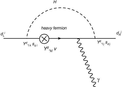
Next, we consider diagrams with heavy fermions and Higgs in the loop (including physical Higgs and longitudinal W/Z bosons). Similar to the previous analysis, we can get the flavor structure of these diagrams from mass insertion approximation. For the purpose of estimating flavor structure, we consider only neutral Higgs diagram (see Fig. 4). From the Yukawa couplings between SM fermion, heavy fermion and Higgs (${\cal{L}}^{\text{SM-Heavy}}$ term of Eq. 15), we find that

$\displaystyle C^{H}_{7\,ij}\propto s_{q_{i}}Y^{d}_{\ast ik}Y^{d}_{\ast kl}Y^{d}_{\ast lj}s_{d_{j}}$

(29)

It is obvious that $C^{H}_{7\,ij}$ is not aligned with $m_{d\,ij}$, assuming no particular structure in the $Y_{\ast}$ (i.e., anarchy). Thus these diagrams will give the leading new contribution to $C_{7}$ and $C^{\prime}_{7}$, and we will focus on these diagrams (see reference [13] for a similar discussion in warped extra dimension).

Because of the near degeneracy of heavy fermion masses, we cannot use mass insertion approximation to calculate the loop diagrams. Instead, we need to diagonalize the $9\times 9$ mass matrix (once we include EWSB-induced mass terms, i.e., coming from Yukawa couplings in Eq. (15)) for all down type quarks in order to determine the mass eigenstates and their couplings. Since it is difficult to obtain an exact analytical formulae for this effect, the analysis is performed numerically in Section 6. However, it is insightful to obtain an approximate analytical formulae for $b\rightarrow s\gamma$ as follows. First, we calculate the dipole operator for the case of one generation quark together with its heavy partners (say, as in the calculation of $(g-2)_{\mu})$) without using the mass insertion approximation and then we simply multiply it by factors from generational mixing effects in order to obtain the amplitude for $b\rightarrow s\gamma$.

In more detail, we diagonalize the $3\times 3$ mass matrix (including the EWSB-induced mass terms) for one generation quarks analytically to first order in $x\equiv Y^{u,d}_{\ast}v/\left(m_{*}\sqrt{2}\right)$ in Appendix B: the results for dipole moment operator of one generation with charged and neutral Higgs in the loop are shown in Eqs. (67) and (71). In order to estimate the effect of mixing between different generations, we again use mass insertion approximation (see Fig. 4). For example, the operator $\bar{b}_{L}\sigma^{\mu\nu}F_{\mu\nu}s_{R}$ can be generated via the mass insertions/Yukawa couplings (as in Eq. 29, but dropping the flavor indices on $Y_{d*}$ for simplicity)

$$Y_{d*}s_{q3}Y_{d*}vY_{d*}s_{d2}$$

(30)

Based on our assumption of anarchy and the formulae for Yukawa couplings and mixing angles (Eq. (15) (20)), we know that

$$Y_{d*}vs_{q3}s_{d2}=Y_{d*}vs_{q3}s_{d3}\frac{s_{d2}}{s_{d3}}\sim m_{b}(D_{R})_{23}$$

(31)

and

$\displaystyle\frac{m_{s}}{m_{b}}$

$\displaystyle\sim$

$\displaystyle\left(D_{L}\right)_{23}\left(D_{R}\right)_{23}$

(32)

In addition, since left-handed down and up-type quarks have the same elementary-composite mixing, we get (again assuming anarchy of $Y_{d\ast}$)

	$\displaystyle\left(D_{L}\right)_{23}$	$\displaystyle\sim$	$\displaystyle\left(U_{L}\right)_{23}$		(33)
		$\displaystyle\sim$	$\displaystyle V_{ts}\;\hbox{or}\;V_{cb}$

where in the second line we have used that $V_{CKM}=U_{L}^{\dagger}D_{L}$. Combining Eq (30) through (33), we can find that generational mixing gives a factor $\sim\frac{m_{s}}{m_{b}V_{ts}}$. Similarly, for the operator $\bar{b}_{R}\sigma^{\mu\nu}F_{\mu\nu}s_{L}$ we have (as in Eq. 29)

$$Y_{d*}s_{d3}Y_{d*}vY_{d*}s_{q2}\sim(Y_{d*})^{2}m_{b}(D_{L})_{23}\sim(Y_{d*})^{2}m_{b}V_{ts}$$

(34)

i.e., generational mixing gives a factor $\sim V_{ts}$. Note that for neutral Higgs diagram the amplitude is proportional to $Y_{d\ast}^{3}$. The flavor structure for charged Higgs (would-be Goldstone) diagram is similar, expect that there are two types of contributions (schematically $\propto Y_{d\ast}^{3}$ and $Y_{u\ast}^{2}Y_{d\ast}$). For simplicity, we set $Y_{u\ast}=Y_{d\ast}\equiv Y_{*}$ in our estimation.

Then, multiplying the one generation results for dipole operator in Eqs. (67) and (71) by the above generational mixing factors, we get the following effective Hamiltonians:

$$\mathcal{H}^{eff}_{\text{charged\, Higgs}}\approx\frac{5}{12}(Y_{*})^{2}m_{b}\frac{ie}{16\pi^{2}}\frac{(2\epsilon\cdot p)}{(m_{*})^{2}}[V_{ts}\bar{b}(1-\gamma_{5})s+\frac{m_{s}}{m_{b}V_{ts}}\bar{b}(1+\gamma_{5})s]$$

(35)

$$\mathcal{H}^{eff}_{\text{neutral\, Higgs}}\approx-\frac{1}{4}(Y_{*})^{2}m_{b}\frac{ie}{16\pi^{2}}\frac{(2\epsilon\cdot p)}{(m_{*})^{2}}[V_{ts}\bar{b}(1-\gamma_{5})s+\frac{m_{s}}{m_{b}V_{ts}}\bar{b}(1+\gamma_{5})s]$$

(36)

We present the results for both charged Higgs and neutral Higgs contribution since they generally have different phase and cannot be simply added together. Since their sizes are of the same order, we will focus just on charged Higgs contribution in the analytical estimates. Then, the new physics contribution to the Wilson coefficients are⁶⁶ 6 Note that such a size for these Wilson coefficients can be estimated, i.e., derived up to $O(1)$ factors, using purely mass insertion approximation. As explained above, here instead we have calculated the $O(1)$ factor from loop diagram (without using mass insertion approximation), although we still used mass insertion approximation to estimate the generational mixing factors.

$\displaystyle C^{2-\text{site}}_{7\;\hbox{estimate}}(m_{*})=-\frac{5}{48}\frac{(Y_{*})^{2}}{(m_{*})^{2}}\frac{\sqrt{2}}{G_{F}};\qquad C^{\,\prime\,2-\text{site}}_{7\;\hbox{estimate}}(m_{*})=-\frac{5}{48}\frac{(Y_{*})^{2}}{(m_{*})^{2}}\frac{\sqrt{2}}{G_{F}}\frac{m_{s}}{m_{b}\lambda^{4}}$

(37)

where we used $V_{ts}\sim\lambda^{2}$ ($\lambda\approx 0.22$). As explained earlier, (based on assumption of anarchy) in the exact result for $b\rightarrow s\gamma$ there will be several terms of the above order but with uncorrelated phases. Thus Eq. (37) is only an estimate for $b\rightarrow s\gamma$, i.e., the natural size of one term that contribute to the new physics effective Hamiltonian. We expect the final result of the coherent sum of such terms to be of the same order as this one-term estimates. From these estimates we can conclude that $C^{\,\prime 2-\text{site}}_{7}(m_{*})$ is bigger than $C^{2-\text{site}}_{7}(m_{*})$ by a factor of $m_{s}/\left(m_{b}V_{ts}^{2}\right)\sim 8$, which is different than the case in SM (where $C^{\,\prime}_{7}\approx C_{7}\;m_{s}/m_{b}$).

As mentioned earlier, in Section 6, we will apply the exact diagonalization of the $9\times 9$ mass matrix for three generations to the results from general loop calculation of $b\rightarrow s\gamma$ in Appendix A to obtain $C_{7}^{2-\text{site}}$ and $C^{\,\prime 2-\text{site}}_{7}$ numerically.

The leading order QCD corrections will suppress the new physics contribution to the Wilson coefficients

$\displaystyle C^{2-\text{site}}_{7}(\mu_{w})=\left[\frac{\alpha_{s}(m_{*})}{\alpha_{s}(m_{t})}\right]^{16/21}\left[\frac{\alpha_{s}(m_{t})}{\alpha_{s}(\mu_{w})}\right]^{16/23}C_{7}^{2-\text{site}}(m_{*})\approx 0.73\ C_{7}^{2-\text{site}}(m_{*})$

(38)

We add it to $C^{\text{SM}}_{7}(\mu_{w})$ in Eq. (26) and then use this sum, i.e., $C^{\text{total}}_{7}(\mu_{w})=C^{\hbox{SM}}_{7}(\mu_{w})+C^{2-\text{site}}_{7}(\mu_{w})$ in Eq. (27) to obtain $C_{7}(\mu_{b})$. Whereas, the SM contribution to $C^{\,\prime}_{7}$ is negligible compared to that in the two-site model so that we have

	$\displaystyle C^{\,\prime\text{total}}_{7}(\mu_{b})$	$\displaystyle\approx$	$\displaystyle C^{\,\prime 2-\text{site}}_{7}(\mu_{b})$		(39)
		$\displaystyle=$	$\displaystyle\left[\frac{\alpha_{s}(m_{*})}{\alpha_{s}(m_{t})}\right]^{16/21}\left[\frac{\alpha_{s}(m_{t})}{\alpha_{s}(\mu_{b})}\right]^{16/23}C^{\,\prime 2-\text{site}}_{7}(m_{*})$
		$\displaystyle\approx$	$\displaystyle 0.48\ C^{\,\prime 2-\text{site}}_{7}(m_{*})$

The contributions from $C_{7}(\mu_{b})$ and $C^{\,\prime}_{7}(\mu_{b})$ sum incoherently (without interference) in the total (i.e., SM and new physics) decay width $\Gamma^{\text{total}}(b\rightarrow s\gamma)$:

$$\Gamma^{\text{total}}(b\rightarrow s\gamma)\propto|C_{7}(\mu_{b})|^{2}+|C^{\,\prime}_{7}(\mu_{b})|^{2}$$

(40)

For convenience, we define $\delta_{7}\equiv C^{2-\text{site}}_{7}(m_{*})/C^{SM}_{7}(\mu_{w})$ and $\delta^{\prime}_{7}\equiv C^{\,\prime\,2-\text{site}}_{7}(m_{*})/C^{SM}_{7}(\mu_{w})$. Adding these new contributions, we have

$$\frac{\Gamma^{\text{total}}(b\rightarrow s\gamma)}{\Gamma^{SM}(b\rightarrow s\gamma)}\approx 1+0.68Re(\delta_{7})+0.11|\delta^{\prime}_{7}|^{2}$$

(41)

The experimental average value for the branching ratio is $BR(b\rightarrow s\gamma)=(352\pm 23\pm 9)\times 10^{-6}$[37]. The theoretical calculation gives $BR(b\rightarrow s\gamma)=(315\pm 23)\times 10^{-6}$[38]. Adding the $2\sigma$ uncertainties by quadrature we find that a $20\%$ deviation from SM prediction is allowed. If we consider the two contributions separately, we will get the bound $|\delta^{\prime}_{7}|\lesssim 1.4$ and Re$(\delta_{7})\lesssim 0.3$. Using Eqs. (37) and (26), the first condition gives

$$m_{*}\gtrsim(0.63)Y_{*}\,\hbox{TeV}$$

(42)

and the second condition gives us a weaker bound. From this rough estimate, we can see the bound on composite mass scale increases with composite Yukawa coupling.

References

- [1] H. Davoudiasl, J. L. Hewett and T. G. Rizzo, Phys. Lett. B 473, 43 (2000) [arXiv:hep-ph/9911262]; A. Pomarol, Phys. Lett. B 486, 153 (2000) [arXiv:hep-ph/9911294]; S. Chang, J. Hisano, H. Nakano, N. Okada and M. Yamaguchi, Phys. Rev. D 62, 084025 (2000) [arXiv:hep-ph/9912498].
- [2] Y. Grossman and M. Neubert, Phys. Lett. B 474, 361 (2000) [arXiv:hep-ph/9912408].
- [3] T. Gherghetta and A. Pomarol, Nucl. Phys. B 586, 141 (2000) [arXiv:hep-ph/0003129].
- [4] L. Randall and R. Sundrum, Phys. Rev. Lett. 83, 3370 (1999) [arXiv:hep-ph/9905221].
- [5] K. Agashe, R. Contino and R. Sundrum, Phys. Rev. Lett. 95, 171804 (2005) [arXiv:hep-ph/0502222].
- [6] K. Agashe and G. Servant, Phys. Rev. Lett. 93, 231805 (2004) [arXiv:hep-ph/0403143] and JCAP 0502, 002 (2005) [arXiv:hep-ph/0411254].
- [7] K. Agashe, A. Delgado, M. J. May and R. Sundrum, JHEP 0308, 050 (2003) [arXiv:hep-ph/0308036].
- [8] K. Agashe, R. Contino and A. Pomarol, Nucl. Phys. B 719, 165 (2005) [arXiv:hep-ph/0412089];
- [9] K. Agashe and R. Contino, Nucl. Phys. B 742, 59 (2006) [arXiv:hep-ph/0510164]; M. Carena, E. Ponton, J. Santiago and C. E. M. Wagner, Nucl. Phys. B 759, 202 (2006) [arXiv:hep-ph/0607106] and arXiv:hep-ph/0701055; R. Contino, L. Da Rold and A. Pomarol, Phys. Rev. D 75, 055014 (2007) [arXiv:hep-ph/0612048]; A. D. Medina, N. R. Shah and C. E. M. Wagner, Phys. Rev. D 76, 095010 (2007) [arXiv:0706.1281 [hep-ph]]; C. Bouchart and G. Moreau, arXiv:0807.4461 [hep-ph].
- [10] K. Agashe, R. Contino, L. Da Rold and A. Pomarol, Phys. Lett. B 641, 62 (2006) [arXiv:hep-ph/0605341].
- [11] A. Delgado, A. Pomarol and M. Quiros, JHEP 0001, 030 (2000) [arXiv:hep-ph/9911252].
- [12] S. J. Huber and Q. Shafi, Phys. Lett. B 498, 256 (2001) [arXiv:hep-ph/0010195].
- [13] K. Agashe, G. Perez and A. Soni, Phys. Rev. D 71, 016002 (2005) [arXiv:hep-ph/0408134].
- [14] C. Csaki, A. Falkowski and A. Weiler, JHEP 0809, 008 (2008) [arXiv:0804.1954 [hep-ph]].
- [15] M. Blanke, A. J. Buras, B. Duling, S. Gori and A. Weiler, arXiv:0809.1073 [hep-ph].
- [16] A. L. Fitzpatrick, G. Perez and L. Randall, arXiv:0710.1869 [hep-ph].
- [17] S. Davidson, G. Isidori and S. Uhlig, Phys. Lett. B 663, 73 (2008) [arXiv:0711.3376 [hep-ph]];
- [18] G. Cacciapaglia, C. Csaki, J. Galloway, G. Marandella, J. Terning and A. Weiler, JHEP 0804, 006 (2008) [arXiv:0709.1714 [hep-ph]]; M. C. Chen and H. B. Yu, arXiv:0804.2503 [hep-ph]; G. Perez and L. Randall, arXiv:0805.4652 [hep-ph]; C. Csaki, C. Delaunay, C. Grojean and Y. Grossman, arXiv:0806.0356 [hep-ph]; J. Santiago, arXiv:0806.1230 [hep-ph]; C. Csaki, Y. Grossman, G. Perez, Z. Surujon and A. Weiler, to appear.
- [19] C. Csaki, A. Falkowski and A. Weiler, arXiv:0806.3757 [hep-ph].
- [20] For studies with TeV KK masses, see S. J. Huber and Q. Shafi, Phys. Lett. B 512, 365 (2001) [arXiv:hep-ph/0104293]; S. J. Huber, Nucl. Phys. B 666, 269 (2003) [arXiv:hep-ph/0303183]; S. Khalil and R. Mohapatra, Nucl. Phys. B 695, 313 (2004) [arXiv:hep-ph/0402225].
- [21] G. Burdman, Phys. Lett. B 590, 86 (2004) [arXiv:hep-ph/0310144]; G. Moreau and J. I. Silva-Marcos, JHEP 0603, 090 (2006) [arXiv:hep-ph/0602155]; K. Agashe, G. Perez and A. Soni, Phys. Rev. D 75, 015002 (2007) [arXiv:hep-ph/0606293]; S. Chang, C. S. Kim and J. Song, JHEP 0702, 087 (2007) [arXiv:hep-ph/0607313] and Phys. Rev. D 77, 075001 (2008) [arXiv:0712.0207 [hep-ph]]; P. M. Aquino, G. Burdman and O. J. P. Eboli, Phys. Rev. Lett. 98, 131601 (2007) [arXiv:hep-ph/0612055]; W. F. Chang, J. N. Ng and J. M. S. Wu, arXiv:0806.0667 [hep-ph] and arXiv:0809.1390 [hep-ph].
- [22] K. Agashe, G. Perez and A. Soni, Phys. Rev. Lett. 93, 201804 (2004) [arXiv:hep-ph/0406101].
- [23] K. Agashe, A. E. Blechman and F. Petriello, Phys. Rev. D 74, 053011 (2006) [arXiv:hep-ph/0606021].
- [24] S. Casagrande, F. Goertz, U. Haisch, M. Neubert and T. Pfoh, arXiv:0807.4937 [hep-ph].
- [25] H. Davoudiasl, B. Lillie and T. G. Rizzo, JHEP 0608, 042 (2006) [arXiv:hep-ph/0508279]; M. Piai, arXiv:hep-ph/0608241; J. Hirn and V. Sanz, JHEP 0703, 100 (2007) [arXiv:hep-ph/0612239]; C. D. Carone, J. Erlich and J. A. Tan, Phys. Rev. D 75, 075005 (2007) [arXiv:hep-ph/0612242].
- [26] G. Cacciapaglia, C. Csaki, G. Marandella and J. Terning, JHEP 0702, 036 (2007) [arXiv:hep-ph/0611358].
- [27] R. Contino, Y. Nomura and A. Pomarol, Nucl. Phys. B 671, 148 (2003) [arXiv:hep-ph/0306259].
- [28] P. McGuirk, G. Shiu and K. M. Zurek, JHEP 0803, 012 (2008) [arXiv:0712.2264 [hep-ph]]; G. Shiu, B. Underwood, K. M. Zurek and D. G. E. Walker, Phys. Rev. Lett. 100, 031601 (2008) [arXiv:0705.4097 [hep-ph]]; A. Falkowski and M. Perez-Victoria, arXiv:0806.1737 [hep-ph]; B. Batell, T. Gherghetta and D. Sword, arXiv:0808.3977 [hep-ph].
- [29] H. Davoudiasl, J. L. Hewett and T. G. Rizzo, Phys. Rev. D 68, 045002 (2003) [arXiv:hep-ph/0212279]; M. Carena, E. Ponton, T. M. P. Tait and C. E. M. Wagner, Phys. Rev. D 67, 096006 (2003) [arXiv:hep-ph/0212307]; M. S. Carena, A. Delgado, E. Ponton, T. M. P. Tait and C. E. M. Wagner, Phys. Rev. D 68, 035010 (2003) [arXiv:hep-ph/0305188]; M. S. Carena, A. Delgado, E. Ponton, T. M. P. Tait and C. E. M. Wagner, Phys. Rev. D 71, 015010 (2005) [arXiv:hep-ph/0410344].
- [30] R. Contino, T. Kramer, M. Son and R. Sundrum, JHEP 0705, 074 (2007) [arXiv:hep-ph/0612180].
- [31] N. Arkani-Hamed, A. G. Cohen and H. Georgi, Phys. Rev. Lett. 86, 4757 (2001) [arXiv:hep-th/0104005]; C. T. Hill, S. Pokorski and J. Wang, Phys. Rev. D 64, 105005 (2001) [arXiv:hep-th/0104035].
- [32] J. M. Maldacena, Adv. Theor. Math. Phys. 2, 231 (1998) [Int. J. Theor. Phys. 38, 1113 (1999)] [arXiv:hep-th/9711200]; S. S. Gubser, I. R. Klebanov and A. M. Polyakov, Phys. Lett. B 428, 105 (1998) [arXiv:hep-th/9802109]; E. Witten, Adv. Theor. Math. Phys. 2, 253 (1998) [arXiv:hep-th/9802150].
- [33] N. Arkani-Hamed, M. Porrati and L. Randall, JHEP 0108, 017 (2001) [arXiv:hep-th/0012148]; R. Rattazzi and A. Zaffaroni, JHEP 0104, 021 (2001) [arXiv:hep-th/0012248].
- [34] A. J. Buras, published in ‘’Probing the Standard Model of Particle Interactions” (Les Houches lectures of 1997), arXiv:hep-ph/9806471.
- [35] M. Bona et al. [UTfit Collaboration], JHEP 0803 (2008) 049 [arXiv:0707.0636 [hep-ph]].
- [36] M. Misiak et al., Phys. Rev. Lett. 98, 022002 (2007) [arXiv:hep-ph/0609232].
- [37]
Heavy Flavor Averaging Group,
http://www.slac.stanford.edu/xorg/hfag/rare/winter08/radll/btosg.pdf - [38] T. Huber, J. Phys. Conf. Ser. 110, 052024 (2008) [arXiv:0712.3158 [hep-ph]].
- [39] K. Agashe, A. Belyaev, T. Krupovnickas, G. Perez and J. Virzi, Phys. Rev. D 77, 015003 (2008) [arXiv:hep-ph/0612015]; B. Lillie, L. Randall and L. T. Wang, JHEP 0709, 074 (2007) [arXiv:hep-ph/0701166]; B. Lillie, J. Shu and T. M. P. Tait, Phys. Rev. D 76, 115016 (2007) [arXiv:0706.3960 [hep-ph]]; A. Djouadi, G. Moreau and R. K. Singh, Nucl. Phys. B 797, 1 (2008) [arXiv:0706.4191 [hep-ph]]; M. Guchait, F. Mahmoudi and K. Sridhar, Phys. Lett. B 666, 347 (2008) [arXiv:0710.2234 [hep-ph]]; U. Baur and L. H. Orr, Phys. Rev. D 76, 094012 (2007) [arXiv:0707.2066 [hep-ph]] and Phys. Rev. D 77, 114001 (2008) [arXiv:0803.1160 [hep-ph]]; M. Carena, A. D. Medina, B. Panes, N. R. Shah and C. E. M. Wagner, Phys. Rev. D 77, 076003 (2008) [arXiv:0712.0095 [hep-ph]].
- [40] K. Agashe et al., Phys. Rev. D 76, 115015 (2007) [arXiv:0709.0007 [hep-ph]]; K. Agashe, S. Gopalakrishna, T. Han, G-Y. Huang and A. Soni, arXiv:0810.1497 [hep-ph].
- [41] E. Lunghi and A. Soni, JHEP 0709, 053 (2007) [arXiv:0707.0212 [hep-ph]]; E. Lunghi and A. Soni, Phys. Lett. B 666, 162 (2008) [arXiv:0803.4340 [hep-ph]]; A. J. Buras and D. Guadagnoli, Phys. Rev. D 78, 033005 (2008) [arXiv:0805.3887 [hep-ph]].
- [42] M. Bona et al. [UTfit Collaboration], arXiv:0803.0659 [hep-ph].
- [43] D. Atwood, M. Gronau and A. Soni, Phys. Rev. Lett. 79, 185 (1997) [arXiv:hep-ph/9704272].
- [44]
http://www.slac.stanford.edu/xorg/hfag/triangle/winter2008/index.shtml#bsgamma - [45] For applications to compact slice of AdS, see, for example, A. Lewandowski, M. J. May and R. Sundrum, Phys. Rev. D 67, 024036 (2003) [arXiv:hep-th/0209050]; A. Lewandowski and M. Redi, Phys. Rev. D 68, 044012 (2003) [arXiv:hep-th/0305013]; A. Lewandowski, Phys. Rev. D 71, 024006 (2005) [arXiv:hep-th/0409192].
- [46] A. Pomarol, Phys. Rev. Lett. 85, 4004 (2000) [arXiv:hep-ph/0005293]; L. Randall and M. D. Schwartz, Phys. Rev. Lett. 88, 081801 (2002) [arXiv:hep-th/0108115] and JHEP 0111, 003 (2001) [arXiv:hep-th/0108114]; W. D. Goldberger and I. Z. Rothstein, Phys. Rev. Lett. 89, 131601 (2002) [arXiv:hep-th/0204160]; Phys. Rev. D 68, 125011 (2003) [arXiv:hep-th/0208060] and Phys. Rev. D 68, 125012 (2003) [arXiv:hep-ph/0303158]; K. Agashe, A. Delgado and R. Sundrum, Nucl. Phys. B 643, 172 (2002) [arXiv:hep-ph/0206099] and Annals Phys. 304, 145 (2003) [arXiv:hep-ph/0212028]; R. Contino, P. Creminelli and E. Trincherini, JHEP 0210, 029 (2002) [arXiv:hep-th/0208002].
- [47] K. w. Choi and I. W. Kim, Phys. Rev. D 67, 045005 (2003) [arXiv:hep-th/0208071].
- [48] H. Davoudiasl, G. Perez and A. Soni, Phys. Lett. B 665, 67 (2008) [arXiv:0802.0203 [hep-ph]].
- [49] T. Appelquist, H. C. Cheng and B. A. Dobrescu, Phys. Rev. D 64, 035002 (2001) [arXiv:hep-ph/0012100].
- [50] K. Agashe, T. Okui and R. Sundrum, arXiv:0810.1277 [hep-ph].