Vortex interactions in a thin platelet superconductor

Thermal fluctuations of vortices, taking into account pinning by impurities and vortex-vortex interactions, is a challenging and technologically important problem in statistical physics. An elegant approach to this subject is to map each fluctating vortex line into the world line of a quantum particle in a Feynman path integral, with the magnetic field direction becoming the imaginary time direction and the bosons moving in the other two spatial directions.[1, 2] Such a mapping is especially powerful for studying columnar defects which become static point defects in the quantum model. When the field direction is tilted relative to the (parallel) pins a novel non-Hermitean 2-dimensional many-body quantum problem arises.[3] If the superconductor is a thin platelet, of thickness of order the penetration depth, with the field lying in the plane, then the quantum bosons are essentially restricted to one dimension. This allows theoretical techniques including Tomonoga Luttinger liquid (TLL) theory and Density Matrix Renormalization Group (DMRG) to be brought to bear,[4, 5] rendering tractible a formidable problem. It may be feasible to realize this classical analogue of a Luttinger liquid experimentally using high-T_c superconductors. A promising candidate would be a very clean highly underdoped YBCO single crystal in which the penetration depth $\lambda_{c}$ can be as large as 50 microns. A platelet should be cleaved with thickness in the $a$-direction of order .1 to 1 mm. and then a magnetic field should be applied in the $b$-direction.

It was shown in [4, 5] that critical phenomena connected with rotating the field direction away from the pin direction is controlled by the dimensionless Luttinger parameter, $g$. In the case $g>1$ columnar defects are irrelevant and have little effect on the long-distance properties of the vortices. On the other hand, for $g<1$ they are relevant and an arbitrarily weak pinning potential drastically alters the system. Thus it is of considerable interest to determine $g$ and how it depends on the parameters of the system, including the density, $n_{0}$. In the dilute limit $g$ approaches unity and the interacting boson system becomes equivalent to non-interacting fermions. The leading density dependent correction is[5]

$$g=1-2an_{0}.$$

(1)

Here $a$ is the 1-dimensional scattering length. This is defined in terms of the 1-dimensional even-channel phase shift, $\delta(k)$. The even wave functions have the asymptotic long-distance behaviour:

$$\psi_{e}(x)\to\sin[k|x|-\delta(k)],$$

(2)

where $x$ is the separation of the 2 bosons. At $k\to 0$ the phase shift is linear in $k$:

$$\delta(k)\to ak,$$

(3)

implying:

$$\psi_{e}(x)\to\sin k(|x|-a).$$

(4)

Thus the relevance or irrelevance of pinning, in the dilute limit is determined by the sign of $a$. It is important to realize that this crucial sign is not fixed by the requirement that the boson-boson interaction be repulsive. For example, an infinite hard core repulsion of range $a_{0}$ leads to a scattering length $a=a_{0}>0$. On the other hand, a repulsive $\delta$-function interaction, $v\delta(x)$, leads to a negative scattering length, $a=-1/(\mu v)$ (where $\mu$ is the reduced mass). In a confined geometry the 1 dimensional scattering length depends not only on the direct inter-particle interaction but also on the effects of the boundaries. This problem was solved by Olshanii[6] for the case of ultra-cold atoms in a harmonic cylindrical trap, where it was shown that the sign of $a$ can be positive or negative depending on the ratio of the (positive) 3 dimensional scattering length to the trap radius.

In this paper we study the properties of two interacting vortices in a thin platelet, or equivalently of 2 interacting bosons restricted to a narrow strip. We begin with the usual modified Bessel-function interaction between vortices given by anisotropic London theory. Standard boundary conditions at the edges of the platelet imply the existence of an infinite set of image vortices for each physical vortex. The interaction of an isolated vortex with its images, and with the external magnetic field determines its wave-function, $f(y)$, in the quantum mechanical analogue, determining the probability of the vortex being at a distance $y$ from the centre of the platelet. It is peaked near the centre, $y=0$. We then consider the scattering of two physical vortices, taking into account the interactions with all image vortices. In general the two vortices could move off centre (away from $y_{1}=y_{2}=0$) as they scatter. Thus the calculation of the effective 1D scattering length requires, in principle, solving for a 2-dimensional 2-body wave-function.

Fortunately, there is a very large dimensionless number that appears quite generally in the thermodynamics of vortices, and which simplifies our calculations considerably. Consider, for simplicity, a macroscopic isotropic London superconductor of penetration depth $\lambda$ and coherence length $\xi$. We approximate the Gibbs free energy for $N$ vortices as:

$$G\approx\int d\tau\left[\tilde{\epsilon}_{1}\sum_{i=1}^{N}\left({d\vec{r}_{i}\over d\tau}\right)^{2}+{\phi_{0}^{2}\over 8\pi^{2}\lambda^{2}}\sum_{i<j}K_{0}(|\vec{r}_{i}(\tau)-\vec{r}_{j}(\tau)|/\lambda)\right].$$

(5)

Here $\phi_{0}=hc/(2e)\approx 2\times 10^{-7}\hbox{G.-cm.}^{2}$ is the flux quantum and

$$\tilde{\epsilon}_{1}\approx{\phi_{0}^{2}\over 16\pi^{2}\lambda^{2}}\ln(\lambda/\xi),$$

(6)

the tilt modulus, is simply the energy per unit length of the vortex.[7] $\tau$ is the spatial co-ordinate along the field direction and $\vec{r}_{i}(\tau)$ describes the shape of the $i^{th}$ vortex. We have approximated the vortex-vortex interaction as only depending on the difference of the $\vec{r}_{i}$’s at the same value of $\tau$ and used the standard London model result for the interaction energy per unit length between straight parallel vortices,[7] given by the modified Bessel function, $K_{0}$. (This needs to be cut off at short distances of order $r_{ij}\approx\xi$.) We approximate the partition function by an integral over vortex paths, $\vec{r}_{i}(\tau)$, weighted by the Boltzmann factor, $\exp[-G/(k_{B}T)]$. By identifying $G/(k_{B}T)$ with $S/\hbar$ where $S$ is the classical action for $N$ interacting bosons, the classical partition function describing thermal fluctuations of vortices becomes equivalent to the Feynman path integral for interacting bosons. In this way various thermal properties of the vortex system can be conveniently obtained from the quantum system.[1, 2] (We set $\hbar$ and $k_{B}=1$.) The corresponding Hamiltonian is:

$$H=-{1\over 2m}\sum_{i=1}^{N}\nabla_{i}^{2}+{\phi_{0}^{2}\over 8\pi^{2}\lambda^{2}T}\sum_{i<j}K_{0}(|\vec{r}_{i}(\tau)-\vec{r}_{j}(\tau)|/\lambda)$$

(7)

with

$$m=\tilde{\epsilon}_{1}/T.$$

(8)

(Strictly speaking, even after inserting appropriate factors of $\hbar$ and $k_{B}$, both terms in this Hamiltonian have dimensions of inverse length rather than energy. This can be traced back to the fact that in Eq. (5) $\tau$ is a spatial coordinate in the classical model but is treated as an imaginary time in the analogue quantum one. This creates no problems for our analysis since physical quantities calculated using this quantum approach involve appropriate ratios of parameters with the correction dimensions, as we shall see.) It is convenient to change to dimensionless length variables, letting:

$$\vec{u}_{i}\equiv\vec{r}_{i}/\lambda.$$

(9)

We then may write the Hamiltonian in dimensionless form:

$$2m\lambda^{2}H=-\sum_{i=1}^{N}\nabla_{i}^{2}+V_{0}\sum_{i<j}K_{0}(|\vec{u}_{i}-\vec{u}_{j}|)$$

(10)

where the dimensionless parameter which measures the interaction strength is:

$$V_{0}={\tilde{\epsilon}_{1}\phi_{0}^{2}\over 4\pi^{2}T^{2}}\approx\left({\phi_{0}^{2}\over 8\pi^{2}T\lambda}\right)^{2}\ln(\lambda/\xi).$$

(11)

Noting that

$$\phi_{0}^{2}/(8\pi^{2}k_{B})=3.9223\times 10^{4}\ \mu\hbox{m}\ -\ \hbox{K}$$

(12)

we see that $V_{0}\gg 1$ for essentially any superconductor at any $T<T_{c}$. This means that the analogue quantum mechanical bosons have very strong short-range interactions when measured in dimensionless units. Variants of this large number will appear when we consider the potential energy function that holds the vortices in the middle of the slab and the interaction between vortices inside the slab. This implies that the vortices stay near the centre of the slab up to rather large slab widths justifying a 1 dimensional approximaton. It also allows an unusual but powerful semi-classical approximation to be applied to the 1 dimensional problem yielding an explicit formula for the scattering length as a function the platelet thickness $d$ and other parameters ($\lambda_{a}$, $\lambda_{c}$, $\xi_{a}$, $\xi_{c}$ and $T$). Our conclusion is that $a$ is positive and large for narrow platelets, increasing with $d$ and having a value $a\approx 19\lambda_{a}$ for $d=10\lambda_{c}\approx.5mm$. This implies that columnar pins are relevant and also that the system rapidly leaves the dilute regime at low densities of order $1/(20\lambda_{a})$, corresponding to fields, $H$ only slightly above $H_{c1}$.

In the next section we briefly review London theory and discuss properties of a single vortex in a thin platelet. In Sec. III we consider 2 interacting vortices, determining the scattering length. Sec. IV contains conclusions.

We make the London approximation,[7] valid when the penetration depth is much longer than the coherence length, $\lambda\gg\xi$. We label the direction perpendicular to the platelet the $y$-direction, and label the direction of the magnetic field the $z$ direction. In a YBCO crystal the most promising geometry may be choosing $y$ and $z$ to be the $a$ and $b$ directions (or vice versa). See Fig. (1). Thus the thin direction of the platelet is the $a$ direction, not the usual growth direction, which is $c$. Such a sample could presumably be obtained by cleaving a macroscopic sample. The magnetic field of a single vortex, centered at $\vec{r}=(x,y)=0$ thus obeys:

$$h-\left[\lambda_{a}^{2}\frac{\partial^{2}h}{\partial x^{2}}+\lambda_{c}^{2}\frac{\partial^{2}h}{\partial y^{2}}\right]=\phi_{0}\delta^{2}(r).$$

(13)

The Dirac $\delta$-function at the vortex core should actually be smeared over a distance of order $\xi$, the coherence length. Note that the decay of the magnetic field in the $x=c$ direction is governed by supercurrents running in the in the $y=a$ direction and hence involves $\lambda_{a}$ whereas the decay in the $y=a$ direction is governed by supercurrents running in the $x=c$ direction and hence involves $\lambda_{c}$. In extremely underdoped YBCO crystals typical parameter values are

	$\displaystyle\lambda_{c}$	$\displaystyle=$	$\displaystyle 50\mu\text{m}$
	$\displaystyle\lambda_{a}$	$\displaystyle=$	$\displaystyle.5\mu\text{m}$
	$\displaystyle\xi_{a}$	$\displaystyle=$	$\displaystyle 5\text{nm}$
	$\displaystyle\xi_{c}$	$\displaystyle=$	$\displaystyle.05\text{nm}$
	$\displaystyle T_{c}$	$\displaystyle=$	$\displaystyle 17K.$		(14)

(The value of $\xi_{c}$ may be a bit small compared to existing measurements but it is convenient to assume the result which follows from anisotropic Ginsburg-Landau theory: $\lambda_{c}/\lambda_{a}=\xi_{a}/\xi_{c}$. In any event our results only depend logarithmically on the $\xi$’s.) Thus the vortex is extremely elliptical: much more extended in the $y=a$ direction. To acheive the two-dimensional limit, we need the sample thickness to be of order the vortex size. (Actually, as we shall see a thickness of up to ten times the vortex size or more is alright.) Thus we can take advantage of the larger $\lambda_{c}$ by cleaving our crystal in the $a$-direction. We will refer to the parameters in Eq. (14) at temperature $T\approx T_{c}$, with $a=y$ the thin direction as the standard parameters. However, our results should also apply at lower temperatures. Note that the vortex wandering that we are concerned with here occurs primarily in the $x=c$ direction. The vortices presumably feel a periodic potential with wave-length given by the lattice constant in the $c$-direction. We will ignore this here. In the dilute limit that we are considering it is not expected to have an important effect.

The solution of Eq. (13) at distances $r\gg\xi$, ignoring for now the boundaries, can be found by using a Fourier transform and is

	$\displaystyle h$	$\displaystyle=$	$\displaystyle\frac{\phi_{0}}{4\pi^{2}}\int_{-\infty}^{\infty}\int_{-\infty}^{\infty}\frac{e^{i(xk_{x}+yk_{y})}}{\lambda_{a}^{2}k_{x}^{2}+\lambda_{c}^{2}k_{y}^{2}+1}dk_{x}dk_{y}$		(15)
		$\displaystyle=$	$\displaystyle\frac{\phi_{0}}{2\pi\lambda_{a}\lambda_{c}}K_{0}\left(\sqrt{\left(\frac{x}{\lambda_{a}}\right)^{2}+\left(\frac{y}{\lambda_{c}}\right)^{2}}\right)$		(16)

where $K_{0}$ is a modified Bessel function.

The energy per unit length of a vortex is

$$\epsilon=-\frac{1}{8\pi}\int h\left[\lambda_{a}^{2}\frac{\partial h}{\partial x}\hat{x}+\lambda_{c}^{2}\frac{\partial h}{\partial y}\hat{y}\right]\cdot d\sigma,$$

(17)

where the integral is taken over an ellipse of radii $\xi_{a}$, $\xi_{c}$ around the vortex core. Thus

$$\epsilon\approx\frac{\phi_{0}^{2}}{16\pi^{2}\lambda_{a}\lambda_{c}}\ln\left(\frac{\lambda_{c}}{\xi_{a}}\right),$$

(18)

to logarithmic accuracy. For the parameters in Eq. (14) we have $\epsilon=10^{-8}\text{erg/cm}.$

We remark that the interaction energy per unit length between 2 straight parallel vortices separated by a vector $\vec{r}$ is simply:

$$U_{12}=\frac{\phi_{0}h_{12}}{4\pi},$$

(19)

where $h_{12}(\vec{r})$ is the magnetic field at the location of one vortex produced by the other, Eq. (16).

We now consider a single straight vortex in an infinite slab, of thickness $d$, extending from $-d/2$ to $d/2$. The presence of boundaries of the superconductor at $y=\pm d/2$, imposes boundary conditions,

$$0=j_{y}={\partial h\over\partial x}.$$

(20)

A vortex at position $y$ in a slab of thickness $d$ creates image vortices with magnetic field in the opposite direction at positions $(2n+1)d-y$ for integral $n$, and creates image vortices with field in the same direction at positions $2nd+y$ for all nonzero integral $n$. Thus the magnetic field at location $(x,y_{2})$ for a vortex at $(0,y_{1})$ is:

	$\displaystyle h(x;y_{2},y_{1})$	$\displaystyle=$	$\displaystyle\frac{\phi_{0}}{2\pi\lambda_{a}\lambda_{c}}\left[\sum_{n=-\infty}^{\infty}K_{0}\left(\sqrt{\left(\frac{x}{\lambda_{a}}\right)^{2}+\left(\frac{2nd+y_{1}-y_{2}}{\lambda_{c}}\right)^{2}}\right)\right.$		(21)
			$\displaystyle\left.-\sum_{n=-\infty}^{\infty}K_{0}\left(\sqrt{\left(\frac{x}{\lambda_{a}}\right)^{2}+\left(\frac{(2n+1)d-y_{1}-y_{2}}{\lambda_{c}}\right)^{2}}\right)\right].$

In addition to the field of the vortex and its images an additional field occurs inside the superconductor when a field $H$ is applied outside of it:

$$h_{1}(y)=H\frac{\cosh(y/\lambda_{c})}{\cosh(d/2\lambda_{c})}.$$

(22)

The magnetic field at the position of the vortex, $(0,y)$ due to all its image vortices is:

$$h_{2}(y)=\frac{\phi_{0}}{2\pi\lambda_{a}\lambda_{c}}\left[-\sum_{n=\pm 1,\pm 3...}K_{0}\left(\frac{nd-2y}{\lambda_{c}}\right)+\sum_{n=\pm 2,\pm 4...}K_{0}\left(\frac{nd}{\lambda_{c}}\right)\right].$$

(23)

The Gibbs free energy depends on the position $y$ of the vortex as:

$$V_{1}(y)=\frac{\phi_{0}}{4\pi}[h_{1}(y)+\frac{1}{2}h_{2}(y)]+\hbox{constant}.$$

(24)

This is plotted in Fig. (2(a)) and (2(b) at $H=H_{c1}$. It has a minimum at $y=0$, large barriers at intermediate $y$ and then appears to diverge to $-\infty$ at $y\to\pm d/2$:

$$V_{1}(y)\to-{\phi_{0}^{2}\over 16\pi^{2}\lambda_{a}\lambda_{c}}\ln[\lambda_{c}/(d\pm 2y)].$$

(25)

This divergence is due to the interaction of the vortex with its image at $y\mp d$. This divergence should actually be cut off at $y\mp d/2$ of order $\xi$ due to corrections to London theory. We take this into account by replacing $K_{0}[(nd-2y)/\lambda_{c}]$ by $K_{0}[(nd-2y)/\lambda_{c}]-K_{0}[(nd-2y)/\xi]$ in Eq. (23). For $H>H_{c1}$, we might expect the true minimum energy to be at $y=0$. This gives the usual formula for $H_{c1}$ for an anistropic superconductor:

$$H_{c1}\approx{4\pi\over\phi_{0}}\epsilon.$$

(26)

where $\epsilon$ is the energy per unit length of a bulk vortex, Eq. (18).

We now turn to a study of thermal fluctuations of a single vortex inside the slab for such an anisotropic superconductor. With the magnetic field along the $b$-axis, the tilt modulus is very different for vortex tilting in the $a=y$ or $c=x$ direction. The elastic energy is written:

$$G_{0}=\int d\tau\left[{\tilde{\epsilon}_{a}\over 2}\left({dy\over d\tau}\right)^{2}+{\tilde{\epsilon}_{c}\over 2}\left({dx\over d\tau}\right)^{2}\right].$$

(27)

Due to the assumed symmetry under rotations in the $a$-$b$ plane, the tilt modulus for tilting in the $a$ direction is just given by the energy per unit length:

$$\tilde{\epsilon}_{a}=\epsilon$$

(28)

where $\epsilon$ is given in Eq. (18). On the other hand, the energy per unit length of a vortex aligned parallel to the $c=x$ axis is much larger, resulting in the tilt modulus[8]

$$\tilde{\epsilon}_{c}={\phi_{0}^{2}\lambda_{c}\over 8\pi^{2}\lambda_{a}^{3}}\ln(\lambda_{c}/\xi)\approx{2\lambda_{c}^{2}\over\lambda_{a}^{2}}\tilde{\epsilon}_{a}.$$

(29)

To this must be added the $y$-dependent free energy:

$$G_{1}=\int d\tau V_{1}[y(\tau)].$$

(30)

Here we have again considered only “instantaneous” interactions between the vortex and its images, at a fixed value of $\tau$. We do not expect this approximation to qualitatively change the long distance physics in the dilute limit. If we consider a very long vortex, in a sample of macroscopic length in the $z=\tau=b$ direction, then the probability of the displacement of the vortex from the centre of the slab having some value $y$ is simply given by $|f(y)|^{2}$ where $f$ is the ground state wave-function of the one-dimensional Hamiltonian:

$$H_{1}=-{1\over 2m_{a}}\left({d\over dy}\right)^{2}+{V_{1}(y)\over T}$$

(31)

with

$$m_{a}\equiv\tilde{\epsilon_{a}\over T}.$$

(32)

It is now convenient to define the dimensionless length variable:

$$\tilde{y}\equiv y/\lambda_{c},$$

(33)

in terms of which:

$$2m_{a}\lambda_{c}^{2}H=-\left({d\over d\tilde{y}}\right)^{2}+V_{0y}\left[-\sum_{n}K_{0}[(2n+1)d/\lambda_{c}-2\tilde{y}]+\ln(\lambda_{c}/\xi_{a}){\cosh(\tilde{y}/2)\over\cosh(d/2\lambda_{c})}\right]$$

(34)

where

$$V_{0y}\equiv{2\tilde{\epsilon}_{a}\phi_{0}^{2}\lambda_{c}\over 16\pi^{2}\lambda_{a}T^{2}}=2\left({\phi_{0}^{2}\over 16\pi^{2}\lambda_{a}T}\right)^{2}\ln\left({\lambda_{c}\over\xi_{a}}\right).$$

(35)

[We have set $H=H_{c1}$ given in Eq. (26).] Since we will choose $d$ of order $\lambda_{c}$, we see that the dimensionless number $V_{0y}$ characterizes the height of the barriers holding the vortex at the center of the platelet. Using the numbers in Eq. (14) and choosing $T=T_{c}$ we find:

$$V_{0y}\approx 10^{8}.$$

(36)

We solve this Schroedinger equation numerically for the groundstate, for $d=10\lambda_{c}$, Fig. [2(c)], finding that the particle makes only very small quantum fluctuations away from $y=0$ due to the huge barriers. For the above parameters we find

$$\sqrt{<y^{2}>}=.01419\lambda_{c}=.001419d.$$

(37)

We should estimate the true critical field, $H_{c1}(d)$ using the ground state energy of the quantum Hamiltonian. If the field is too low the particle can tunnel through the barrier corresponding to a vortex terminating at some value of $\tau$ with the magnetic flux leaving the superconductor. However, due to the exceedingly high barrier, the tunnelling probability is miniscule and the system will not be very sensitive to the precise value of $H$. We should also remark that, to solve the Schroedinger equation precisely we need to specifiy some boundary conditions on the wave-function at $y=\pm d/2$. We imposed vanishing boundary conditions. Fortunately, the extremely large dimensionless barrier also renders our results very insensitive to this choice.

Consider two straight parallel vortices inside the platelet, at locations $(x_{i},y_{i})$. The Gibbs free energy per unit length is:

$$V(x_{1}-x_{2};y_{1},y_{2})={\phi_{0}\over 4\pi}h(x_{1}-x_{2};y_{1},y_{2})+V_{1}(y_{1})+V_{2}(y_{2}).$$

(38)

By translational invariance in the $x$-direction, $V$ depends only on the difference of the $x$-coordinates of the two vortices:

$$x\equiv x_{1}-x_{2}.$$

(39)

Here $h(x,y_{1},y_{2})$ is given in Eq. (21) and $V_{1}(y)$ by Eq. (24). The first term in Eq. (38) represents the interaction of one vortex with the other one and with the images of the other one. The second and third terms represent the interaction of each vortex with its own images and with the screened external field. $V(x,y_{1},y_{2})$ has a deep minimum at $y_{1}=y_{2}=0$ for large $|x|\gg\lambda_{a}$. $V(x,0,0)$ has a large peak centred at $x=0$ with a weak, logarithmic divergence right at $x=0$. This logarithmic divergence should be cut off at scales of order $\xi$; however this cut off has essentially no effect on the scattering length, as we shall see.

Again we may study the thermodynamics of two wiggling vortices in the platelet by mapping onto a quantum mechanics model. We make the fundamental assumption that the vortices only bend on long length scales (compared to $\lambda_{a}$) and that we may approximate the vortex-vortex (and vortex-image vortex) interaction by an “instantaneous” one at a fixed value of $\tau=z$. The Boltzmann sum is now over the configuration of two vortices and we must include the vortex-vortex interaction in the free energy. Again identifying the free energy with the imaginary time action, we see that the corresponding quantum Hamiltonian is:

$$H=-{1\over 2}\sum_{i=1}^{2}\left[{1\over m_{a}}\left({d\over dy_{i}}\right)^{2}+{1\over m_{c}}\left({d\over dx_{i}}\right)^{2}\right]+{V(x,y_{1},y_{2})\over T}.$$

(40)

Here $m_{a}$ is given in Eq. (32) and

$$m_{c}\equiv{\tilde{\epsilon}_{c}\over T}$$

(41)

where $\tilde{\epsilon}_{c}$ is given in Eq. (29). In the quantum analogue, the vortices obey Bose statistics[1] and consequently the two-body wave-function must be symmetric: even under $x\to-x$. The asymptotic behavior of the low energy wave-functions at $|x|\gg\lambda_{a}$ is given by:

$$\psi(x,y_{1},y_{2})\to f(y_{1})f(y_{2})\sin[k|x|-\delta(k)]$$

(42)

where $f(y)$ is the ground state wave-function for a single vortex, discussed in Sec. II. The energy of this scattering state is:

$$E=2E_{1}+{k^{2}\over 2\mu}$$

(43)

where $E_{1}$ is the ground state energy for a single vortex, discussed in the previous section and the reduced mass which governs the relative motion is

$$\mu=m_{c}/2.$$

(44)

The scattering length is defined by Eq. (3).

It turns out that, due to the large barrier near $x=0$, for small $y_{i}$, the scattering length is determined almost completely by the large $x$ asymptotic form of the potential, until $d$ gets very large compared to $\lambda_{c}$. The $x$-dependent part of the exact potential can be written as a sum of exponentials:

$$V(x;y_{1},y_{2})=\frac{\phi_{0}^{2}}{4\pi\lambda_{a}^{2}d}\sum_{n=1}^{\infty}f\left(n,\frac{y_{1}}{d},\frac{y_{2}}{d}\right)\frac{e^{-|x|\sqrt{1+(n\pi\lambda_{c}/d)^{2}}/\lambda_{a}}}{\sqrt{1+(n\pi\lambda_{c}/d)^{2}}/\lambda_{a}}+V_{1}(y_{1})+V_{1}(y_{2}).$$

(45)

where we define

$$f(n,y_{1}/d,y_{2}/d)\equiv\left\{\begin{array}[]{rl}\cos(n\pi y_{1}/d)\cos(n\pi y_{2}/d)&\text{if $n$ is odd}\\ \sin(n\pi y_{1}/d)\sin(n\pi y_{2}/d)&\text{if $n$ is even}\end{array}.\right.$$

(46)

At large $|x|$ we may approximate the sum by the first term only:

$$V\approx\frac{\phi_{0}^{2}\lambda}{4\pi\lambda_{a}^{2}d}e^{-|x|/\lambda}\cos(\frac{\pi y_{1}}{d})\cos(\frac{\pi y_{2}}{d})+V_{1}(y_{1})+V_{1}(y_{2})$$

(47)

where we have defined, for convenience, a reduced value of $\lambda_{a}$:

$$\lambda\equiv\lambda_{a}\left[1+\left(\frac{\pi\lambda_{c}}{d}\right)^{2}\right]^{-1/2}.$$

(48)

For this approximation to hold, we need that the first term dominates all other terms. In the one-dimensional limit (i.e. $y_{1}=y_{2}=0$) the condition for large $x$ is

$$\exp\left(\frac{|x|}{\lambda_{a}}\frac{4\pi^{2}\lambda_{c}^{2}}{d^{2}}\right)\gg 1.$$

(49)

Note that, unlike the direct vortex-vortex interaction, this potential has a simple exponential dependence on $x$ at large $|x|$ albeit with a reduced penetration depth.

Due to the large barriers in $V_{1}(y)$ we expect the low energy scattering states to be confined to $y_{i}\approx 0$. We first calculate $a$ assuming that the vortices stay exactly in the middle of the slab, $y_{i}=0$ throughout the scattering process. We return to a further discussion of why this is reasonable at the end of this section. This reduces the problem to a one-dimensional quantum mechanics model with Hamiltonian:

$$H=-{1\over 2\mu}{d^{2}\over dx^{2}}+{V(x)\over T}$$

(50)

where

$$V(x)=V(x;0,0)\to\frac{\phi_{0}^{2}\lambda}{4\pi\lambda_{a}^{2}d}e^{-|x|/\lambda}.$$

(51)

We look for parity even solutions of this Schroedinger equation with asymptotic behavior $\psi(x)\to\sin[k|x|-\delta(k)]$ with $\delta(k)\to ak$ as $k\to 0$. Note that in the small $k$ limit, $\psi(x)\to\sin[k(|x|-a)]$ for $x\gg\lambda$. Then, if we consider an intermediate range of $x$:

$$\lambda\ll|x|\ll 1/k,$$

(52)

we may approximate the wave-function by a linear form:

$$\psi(x)\propto|x|-a.$$

(53)

Thus, to find the scattering length we need to simply solve the zero energy Schroedinger equation:

$$\left[-{1\over 2\mu}{d^{2}\over dx^{2}}+{V(x)\over T}\right]\psi=0.$$

(54)

Note that this reduces the eigenvalue problem to a simple initial value problem. We simply impose the initial conditions:

	$\displaystyle{d\psi\over dx}(0)$	$\displaystyle=$	$\displaystyle 0$
	$\displaystyle\psi(0)$	$\displaystyle=$	$\displaystyle 1$		(55)

and solve the zero energy equation. The asymptotic behavior of the solution at $|x|\gg\lambda$ is given by Eq. (53) which determines the scattering length, $a$.

It is convenient to introduce a dimensionless length variable:

$$\tilde{x}\equiv x/\lambda$$

(56)

in terms of which the Schroedinger equation becomes, at large $|\tilde{x}|$:

$$\left[-{d^{2}\over d\tilde{x}^{2}}+V_{0x}e^{-\tilde{x}}\right]\psi(\tilde{x})=2\mu\lambda^{2}E\psi(\tilde{x}).$$

(57)

Here the dimensionless number which measures the strength of the repulsive potential is:

$$V_{0x}={\tilde{\epsilon}_{c}\phi_{0}^{2}\lambda^{3}\over 4\pi\lambda_{a}^{2}dT^{2}}={1\over 2\pi}\left({\phi_{0}^{2}\over 4\pi\lambda_{a}T}\right)^{2}\ln(\lambda_{c}/\xi_{a}){\lambda_{c}/d\over[1+(\pi\lambda_{c}/d)^{2}]^{3/2}}.$$

(58)

Using our estimates of the parameters in Eq. (14) with $T=T_{c}$ and $d=10\lambda_{c}$ we find:

$$V_{0x}=1.07\times 10^{8}.$$

(59)

Note that $V_{0x}\propto 1/d$ at $d\gg\lambda_{c}$. Importantly $V_{0x}\gg 1$ when $d$ is of order $\lambda_{c}$ and remains large out to extremely large values of $d/\lambda_{c}$. The largeness of $V_{0x}$ leads to a large scattering length, allows for an unusual semi-classical solution approximation and also helps to justify setting $y_{i}=0$ as we shall see below. It is of course, possible to solve the Schroedinger equation numerically for specified values of the parameters. However, the largeness of $V_{0x}$ and $V_{0y}$ creates numerical difficulties for standard algorithms, when one attempts to solve the full 3-dimensional problem, including the $y_{i}$. In this case it is much easier, and more transparent, to use the semi-classical approximation.

Our semi-classical approximation for the scattering length at $V_{0x}\gg 1$ begins with the observation that the classical turning point for 2 particles approaching each other with a small relative momentum, $k$ occurs at $\tilde{x}\gg 1$. Therefore $a$ is determined almost completely by the large $\tilde{x}$ form of the potential in Eq. (47). Using the large $\tilde{x}$ form of the potential, we may solve the one-dimensional Schroedinger equation exactly. To do this we change variables to:

$$u=2\sqrt{V_{0x}}e^{-|\tilde{x}|/2}.$$

(60)

The zero energy Schroedinger equation, (54), simplifies to

$$u^{2}\psi^{\prime\prime}+u\psi^{\prime}-u^{2}\psi=0$$

(61)

where the primes denote differentiation with respect to $u$. This is the zeroth order modified Bessel’s differential equation, and the general solution is given in terms of the modified Bessel functions:

	$\displaystyle\psi$	$\displaystyle=$	$\displaystyle c_{1}I_{0}(u)+c_{2}K_{0}(u)$		(62)
		$\displaystyle=$	$\displaystyle c_{1}I_{0}(2\sqrt{V_{0x}}e^{-|x|/2\lambda})+c_{2}K_{0}(2\sqrt{V_{0x}}e^{-|x|/2\lambda}).$

For large $u$ (i.e. $\tilde{x}<<\ln V_{0}$) we have

$$\psi\approx\frac{1}{\sqrt{2\pi u}}\left(c_{1}e^{u}+c_{2}\pi e^{-u}\right),$$

(63)

or writing in terms of the original variables and putting back factors of $\lambda$, we have

$$\psi\approx\frac{1}{\sqrt{4\pi}V_{0x}^{1/4}e^{-|x|/4\lambda}}\left(c_{1}e^{2\sqrt{V_{0x}}e^{-|x|/2\lambda}}+c_{2}\pi e^{-2\sqrt{V_{0x}}e^{-|x|/2\lambda}}\right)$$

(64)

On the other hand, for small $u$ (i.e. $\tilde{x}>>\ln V_{0}$) we have

$$\psi\approx c_{1}-c_{2}(\ln(u/2)+\gamma)=c_{1}+c_{2}\left(\frac{|\tilde{x}|}{2}-\frac{1}{2}\ln V_{0x}-\gamma\right)$$

(65)

where $\gamma\approx 0.5772$ is the Euler-Mascheroni constant. Note that the last formula can be written as

$$\psi\approx\frac{c_{2}}{2\lambda}(|x|-a)$$

(66)

where the scattering length $a$ is (putting back factors of $\lambda$)

$$a=\lambda(\ln V_{0x}+2\gamma-2c_{1}/c_{2}).$$

(67)

To determine $c_{1}/c_{2}$ we match our solution in the region $1\ll|\tilde{x}|\ll\ln V_{0x}$ to the WKB solution which works for $|x|$ not too large, in the region where $V(x)$ is large. The even WKB wave function for $E=0$ is given by

$$\psi(x)=A\left\{\exp\left[\int_{0}^{x}\sqrt{V^{\prime}(x^{\prime})}dx^{\prime}\right]+\exp\left[-\int_{0}^{x}\sqrt{V^{\prime}(x^{\prime})}dx^{\prime}\right]\right\}$$

(68)

where

$$V^{\prime}(x)=2\mu V(x;0,0)$$

(69)

and $V$ is the exact potential of Eq. (38). (Note that we do not make any large $x$ approximation to $V$ now.) We can rewrite this as

$$\psi(x)=A\left\{e^{-\alpha}\exp\left[\int_{x}^{\infty}\sqrt{V^{\prime}(x^{\prime})}dx^{\prime}\right]+e^{\alpha}\exp\left[-\int_{x}^{\infty}\sqrt{V^{\prime}(x^{\prime})}dx^{\prime}\right]\right\}$$

(70)

where

$$\alpha=\int_{0}^{\infty}\sqrt{V^{\prime}(x)}dx.$$

(71)

Now, if $x$ is large enough for our asymptotic expression $V^{\prime}(x)\approx V_{0x}e^{-x/\lambda}/\lambda^{2}$ to hold, then the integral can be done quite readily:

$$\psi(x)=A\left\{e^{-\alpha}\exp\left[2\sqrt{V_{0x}}e^{-x/2\lambda}\right]+e^{\alpha}\exp\left[-2\sqrt{V_{0x}}e^{-x/2\lambda}\right]\right\}.$$

(72)

Comparison with Eq. (64) thus gives

$$c_{1}/c_{2}=\pi e^{-2\alpha}=\pi\exp\left[-\int_{-\infty}^{\infty}\sqrt{V^{\prime}(x)}dx\right].$$

(73)

This quantity is exponentially small in the large quantity $V_{0x}$ so it is completely negligible. Note also that the logarithmic divergence of $V(x;0,0)$ at $x\to 0$ has no important effects, leaving the integral finite in Eq. (73). The last term in Eq. (67)essentially vanishes, and we simply have that

$$a=\lambda(\ln V_{0x}+2\gamma).$$

(74)

Asymptotically, the scattering length is linearly dependent on the logarithm of the size of the potential.

Interestingly, we get almost the same result for the odd wave functions, except that the sign of $c_{1}/c_{2}$ is reversed. The even channel and odd channel scattering lengths are therefore almost exactly the same. However, it is the difference between the even and odd channel scattering lengths that determines the transmission coefficient, and it is only then that $c_{1}/c_{2}$ plays an important role.

We have based this approximation on the assumption that there exists a region of separation $x$, such that the approximation Eq. (64) holds, and the WKB approximation to the wave function also holds. Typically the matching is done around the region $x\approx a$; therefore we need that (using Eq. (74) and Eq. (49), and noticing $\lambda\approx\lambda_{a}$ for large $d$)

$$\exp\left[\left(\frac{2\pi\lambda_{c}}{d}\right)^{2}\ln(e^{2\gamma}V_{0x})\right]\gg 1$$

(75)

This is the condition that must be satisfied for the formula Eq. (74) to hold.

The wave-function calculated numerically to high precision (in the 1-dimensional approximation) and the semi-classical wave function are compared in Fig. (3) for our standard parameters and $d=10\lambda_{a}$.As can be seen, the two wave functions give good agreement in the large-$x$ regime (with an error $<1\%$ for $x>18\lambda_{a}$). The semi-classical wave function is grossly inaccurate in the small-$x$ region ($x<15\lambda_{a}$) but the wave-function is neglegible there anyway. The predicted semi-classical scattering length is $a=\lambda(\ln V_{0}+2\gamma)=18.7398\lambda_{a}$. The actual scattering length of the numerically determined wave function (obtained by fitting the wave function in the large-$x$ regime to a linear function) is $18.7409\lambda_{a}$. The semi-classical wave function gives an error of less than $0.01\%$. In Fig. (4) we show the scattering length versus $d$, comparing our numerical results to the semi-classical approximation (in both cases making the 1-dimensional approximation). Most of the $d$-dependence in our semi-classical formula, Eq. (74), arises from the $d$-dependence of the reduced penetration depth, $\lambda$, given in Eq. (48). As the sample thickness decreases, the effective range of the interaction potential, $\lambda$, also decreases, and the scattering length simply scales with it, up to logarithmic corrections coming from $V_{0x}$, defined in Eq. (58). The semi-classical and numerical values agree within $1\%$ up to about $d=22\lambda_{c}$. For $d=22\lambda_{c}$, we have that (refer to Condition (75))

$$\left(\frac{2\pi\lambda_{c}}{d}\right)^{2}\ln(e^{2\gamma}V_{0x})=1.56$$

(76)

which is already not far from unity. There will therefore be significant deviations of the true value from Eq. (74). We could also notice that the scattering length tends towards a finite value for large $d$. This is because as the thickness of the sample grows, the image vortices move farther away from the orginal vortices until their effects become negligible.

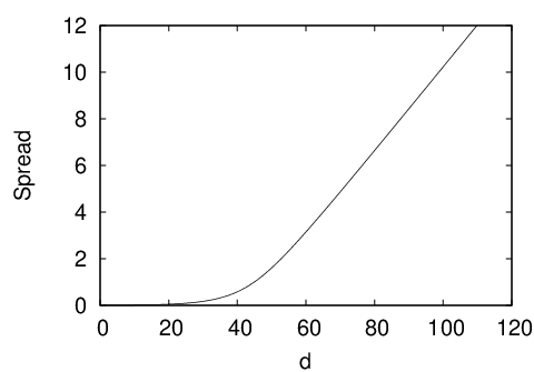
Next, we discuss the validity of our 1-dimensional approximation, setting $y_{i}=0$, which is justified by the fact that the single vortex wave-function, $f(y)$ is so sharply peaked near $y=0$. If we look at the shape of the potentials, $V_{1}(y)$, we see that for small $d$ (Fig. (2(a))) the potential has an obvious minimum in the center, and is approximately simple harmonic near the center. For larger $d$ (Fig. (2(b))), however, the potential is almost negligible except for a large potential barrier close to (but not at) the edges; the potential will be qualitatively more similar to a square well. Therefore as $d$ increases, we would expect the shape of the wave function to morph from a confined Gaussian to a spread-out sinusoidal (Fig. (2(c)), Fig. (2(d))). The spread of the single-vortex wave function ($\langle y^{2}\rangle^{1/2}$) is plotted in Fig. (5). The thickness reaches $1\%$ of the platelet thickness at around $d=35\lambda_{c}$, an indication that our one-dimensional approximation fails above this value. The fact that the thickness becomes linearly dependent on $d$ at large $d$ also suggests that the wave function tends to a fixed shape (a sinusoidal).

A more systematic approximation to solving the full 2-body 2-dimensional Schroedinger equation of Eq. (40), would be to write:

$$\psi(x;y_{1},y_{2})\approx\psi_{1}(x)f(y_{1})f(y_{2})$$

(77)

where $\psi_{1}(x)$ is the 1-dimensional wave-function found above and $f(y_{1})$ is the single vortex wave-function. We could then improve our estimate of the 1-dimensional effective potential by using:

$$V(x)\approx\int dy_{1}dy_{2}|f(y_{1})|^{2}|f(y_{2})|^{2}V(x;y_{1},y_{2})$$

(78)

rather than simply $V(x)\approx V(x;0,0)$. However, because $f(y)$ is so sharply peaked at $y\approx 0$ this makes a negligible difference.

Note that our calculation of $a$ depended essentially only on $V(x)$ in the large $x$ region, $x\gg\lambda$. Our consideration of the small $x$ region only served to determined $c_{1}/c_{2}$ which was exponentially small anyway and can simply be ignored. In this large $x$ region, Eq. (47) is a good approximation, the wave-function approximately factorizes and the large barriers in $V_{1}(y)$ ensure that the wave-function is strongly peaked near $y_{i}=0$. For smaller values of $x$ the wave-function presumably spreads out more in the $y$ direction. However, at smaller $x$ the wave-function is exponentially small anyway.

Finally, we consider the case where the thin direction of the YBCO platelet is the $c$ direction: y=c (and x=a, z=b). In this case the roles of $\lambda_{a}$ and $\lambda_{c}$ are switched, as are the roles of $\tilde{\epsilon}_{a}$ and $\tilde{\epsilon}_{c}$ and we get

	$\displaystyle V_{0y}$	$\displaystyle=$	$\displaystyle 2{\tilde{\epsilon}_{c}\phi_{0}^{2}\lambda_{a}\over 16\pi^{2}T^{2}\lambda_{c}}=4\left({\phi_{0}^{2}\over 16\pi^{2}\lambda_{a}T}\right)^{2}\ln(\lambda_{c}/\xi_{a})$
	$\displaystyle V_{0x}$	$\displaystyle=$	$\displaystyle{\tilde{\epsilon}_{a}\phi_{0}^{2}\lambda^{3}\over 4\pi\lambda_{c}^{2}dT^{2}}={1\over 4\pi}\left({\phi_{0}^{2}\over 4\pi\lambda_{a}T}\right)^{2}\ln(\lambda_{c}/\xi_{a}){\lambda_{a}/d\over[1+(\pi\lambda_{a}/d)^{2}]^{3/2}}$		(79)

where we now define:

$$\lambda\equiv\lambda_{c}\left[1+\left({\pi\lambda_{a}\over d}\right)^{2}\right]^{-1/2}.$$

(80)

Apart from some unimportant factors of $2$, the formulas for $V_{0y}$ and $V_{0x}$ are the same as for the other geometry except that $d$ now appears in the dimensionless ratio $\lambda_{a}/d$ rather than $\lambda_{c}/d$. So we now conclude that the 1 dimensional approximation holds for $d\leq 20\lambda_{a}\approx 10\mu$m. and the semi-classical approximation holds out to roughly the same value of $d$.

Our main result is the formula Eq. (74) for the scattering length. This is plotted versus the platelet thickness, $d$, for our standard parmeters, in Fig. (4). Note that $a$ is everywhere positive and $a/\lambda_{a}$ is everywhere quite large, having the value $a/\lambda_{a}\approx 19$ at $d\approx 10\lambda_{c}$. At somewhat larger values of $d$ we expect our semi-classical approximation to the one-dimensional problem to break down and, more problematically, the one-dimensional approximation itself to start to fail.

The main use of our formula for $a$ is not, of course, for studying the system with only 2 vortices, but rather for studying the thermodynamic limit of many vortices. In the dilute limit, $n_{0}a\ll 1$ (where $n_{0}$ is the vortex density per unit length), $a$ determines the Luttinger parameter via Eq. (1). Of course the Luttinger liquid treatment of the problem assumes that it is fundamentally 1-dimensional. Our calculations here indicate that the 1-dimensional approximation should be good, at least in the dilute limit $n_{0}a\ll 1$, up to platelet thicknesses of order $d=10\lambda_{c}$ or more, since the vortices stay very close to the centre of the platelet. Furthermore, we have determined the Luttinger parameter for this range of thicknesses and vortex densities. When $a$ is large the Luttinger parameter decreases rapidly for increasing vortex density. It was argued in (5) that, at high densites, $g\ll 1$. Taken together, these results suggest a rapid monotonic drop of $g$ from $1$ with increasing density. In this case, columnar pins would be highly relevant for essentially all fields above $H_{c1}$. Thus a promising region to look at experimentally might be very close to $H_{c1}$ with low vortex densities, $n_{0}\ll 1/\lambda_{a}$ and samples of thickness around $10\lambda_{c}$.