跳到论文正文
W Papers独立论文阅读器 arXiv:0810.0261 论文正文 计算阅读时间 · 0%
引用这篇论文根据当前论文元数据生成,正式投稿前建议核对。


License: arXiv.org perpetual non-exclusive license
arXiv:0810.0261v2 [math.GT] 08 Oct 2008

The asymptotic behavior of least pseudo-Anosov dilatations

Chia-yen Tsai
Abstract

For a surface SS with nn marked points and fixed genus g≥2g\geq 2, we prove that the logarithm of the minimal dilatation of a pseudo-Anosov homeomorphism of SS is on the order of log⁡nn\frac{\log n}{n}. This is in contrast with the cases of genus zero or one where the order is 1n\frac{1}{n}.

1 Introduction

Let S=Sg,nS=S_{g,n} be an orientable surface with genus gg and nn marked points. The mapping class group of SS is defined to be the group of homotopy classes of orientation preserving homeomorphisms of SS. We denote it as Mod⁡(S)\mathrm{Mod}(S). Given f∈Mod⁡(S)f\in\mathrm{Mod}(S) a pseudo-Anosov element, let λ⁡(f)\lambda(f) denote the dilatation of ff; see section 2.1. We define

ℒ⁡(Sg,n):={log⁡λ⁡(f)|f∈Mod⁡(Sg,n)​ pseudo-Anosov }.\displaystyle{\cal L}(S_{g,n}):=\{\log\lambda(f)|f\in\mathrm{Mod}(S_{g,n})\text{ pseudo-Anosov }\}.

This is precisely the length spectrum of the moduli space ℳg,n{\cal M}_{g,n} of Riemann surfaces of genus gg with nn marked points with respect to the Teichmuller metric; see [Iva88]. There is a shortest closed geodesic and we denote its length

lg,n=min⁡{log⁡λ⁡(f)|f∈Mod⁡(Sg,n)​ pseudo-Anosov}.\displaystyle l_{g,n}=\min\{\log\lambda(f)|f\in\mathrm{Mod}(S_{g,n})\text{ pseudo-Anosov}\}.

Our main theorem is the following:

Theorem 1.1.

For any fixed g≥2g\geq 2, there is a constant cg≥1c_{g}\geq 1 depending on gg such that

log⁡ncg​n<lg,n<cg​log⁡nn,\displaystyle\frac{\log n}{c_{g}n}<l_{g,n}<\frac{c_{g}\log n}{n},

for all n≥3n\geq 3.

To contrast with known results, we recall that in [Pen91], Penner proves for 2​g−2+n>02g-2+n>0 and n≥0n\geq 0,

lg,n≥log⁡212​g−12+4​n,\displaystyle l_{g,n}\geq\frac{\log 2}{12g-12+4n},

and for closed surfaces

log⁡212​g−12≤lg,0≤log⁡11g.\displaystyle\frac{\log 2}{12g-12}\leq l_{g,0}\leq\frac{\log 11}{g}.

The bounds on lg,0l_{g,0} have been improved by a number of authors; [Bau92], [McM00], [Min06],[HK06].

In [Pen91], Penner suggests that there may be an “analogous upper bound for n≠0n\neq 0”. In [HK06], Hironaka and Kin use a concrete construction to prove that for genus g=0g=0

l0,n<log⁡(2+3)⌊n−22⌋≤2​log⁡(2+3)n−3,\displaystyle l_{0,n}<\frac{\log(2+\sqrt{3})}{\left\lfloor\frac{n-2}{2}\right\rfloor}\leq\frac{2\log(2+\sqrt{3})}{n-3},

for all n≥4n\geq 4. The inequality is proven for even nn in [HK06], but it follows for odd nn by letting the fixed point of their example be a marked point. Combining this with Penner’s lower bound, one sees for n≥4n\geq 4

log⁡24​n−12≤l0,n<2​log⁡(2+3)n−3,\displaystyle\frac{\log 2}{4n-12}\leq l_{0,n}<\frac{2\log(2+\sqrt{3})}{n-3},

which shows that the upper bound is on the same order as Penner’s lower bound for g=0g=0. A similar situation holds for g=1g=1; see the Appendix.

Inspired by the construction of Hironaka and Kin, we tried to find examples of pseudo-Anosov fg,n∈Mod⁡(Sg,n)f_{g,n}\in\mathrm{Mod}(S_{g,n}) with log⁡λ⁡(fg,n)=O⁡(1g+n)\log\lambda(f_{g,n})=O(\frac{1}{g+n}). However for any fixed g≥2g\geq 2, all attempts resulted in fg,n∈Mod⁡(Sg,n)f_{g,n}\in\mathrm{Mod}(S_{g,n}) pseudo-Anosov with log⁡λ⁡(fg,n)=Og​(log⁡nn)\log\lambda(f_{g,n})=O_{g}(\frac{\log n}{n}) and not O⁡(1c⁡(g,n))O(\frac{1}{c(g,n)}) for any linear function c⁡(g,n)c(g,n). This led us to prove Theorem 1.1.

1.1 Outline of the paper

We will first recall some definitions and properties in section 2. In section 3 we prove the lower bound of Theorem 1.1. We construct examples in section 4 which give an upper bound for the genus 22 case, and we extend the example to arbitrary genus g≥2g\geq 2 to obtain the upper bound of Theorem 1.1. Finally, we construct a pseudo-Anosov element in Mod⁡(S1,2​n)\mathrm{Mod}(S_{1,2n}) and obtain an upper bound on l1,2​nl_{1,2n} in the Appendix.

Acknowledgements.

The author would like to thank Christopher Leininger for key discussions and for revising an earlier draft. Kasra Rafi and A.J. Hildebrand offered helpful suggestions and insights. I would also like to thank MSRI for its stimulating, collaborative research environment during its fall 2007 programs.

2 Preliminaries

2.1 Homeomorphisms of a surface

We say that a homeomorphism f:S→Sf:S\rightarrow S is pseudo-Anosov if there are transverse singular foliations ℱs{\cal F}^{s} and ℱu{\cal F}^{u} together with transverse measures μs\mu^{s} and μu\mu^{u} such that for some λ>1\lambda>1

f⁡(ℱs,μs)\displaystyle f({\cal F}^{s},\mu^{s}) =(ℱs,λ​μs),\displaystyle=({\cal F}^{s},\lambda\mu^{s}),
f⁡(ℱu,μu)\displaystyle f({\cal F}^{u},\mu^{u}) =(ℱu,λ−1​μu).\displaystyle=({\cal F}^{u},\lambda^{-1}\mu^{u}).

The number λ=λ⁡(f)\lambda=\lambda(f) is called the dilatation of ff. We call ff reducible if there is a finite disjoint union UU of simple essential closed curves on SS such that ff leaves UU invariant. If there exists k>0k>0 such that fkf^{k} is the identity, then ff is periodic. A mapping class [f][f] is pseudo-Anosov, reducible or periodic (respectively) if ff is homotopic to a pseudo-Anosov, reducible or periodic homeomorphism (respectively). The following is proved in [FLP91].

Theorem 2.1.

(Nielsen-Thurston) A mapping class [f]∈M​o​d​(S)[f]\in Mod(S) is either periodic, reducible, or pseudo-Anosov.

As a slight abuse of notation, we sometimes refer to a mapping class [f][f] by one of its representatives ff.

2.2 Markov partitions

Suppose f:S→Sf:S\rightarrow S is pseudo-Anosov with stable and unstable measured singular foliations (ℱs,μs)({\cal F}^{s},\mu^{s}) and (ℱu,μu)({\cal F}^{u},\mu^{u}). We define a rectangle RR to be a map ρ:I×I→S\rho:I\times I\rightarrow S such that ρ\rho is an embedding on the interior, ρ⁡(p​o​i​n​t×I)\rho(point\times I) is contained in a leaf of ℱu{\cal F}^{u}, and ρ⁡(I×p​o​i​n​t)\rho(I\times point) is contained in a leaf of ℱs{\cal F}^{s}. We denote ρ⁡(∂I×I)\rho(\partial I\times I) by ∂uR\partial^{u}R and ρ⁡(I×∂I)\rho(I\times\partial I) by ∂sR\partial^{s}R.

[Uncaptioned image]

As a standard abuse of notation, we will write R⊂SR\subset S for the image of a rectangle ρ:I×I→S\rho:I\times I\rightarrow S.

Definition 2.2.

A Markov partition for f:S→Sf:S\rightarrow S is a decomposition of SS into a finite union of rectangles {Ri}i=1k\{R_{i}\}_{i=1}^{k}, such that:

  1. 1.

    I​n​t​(Ri)∩I​n​t​(Rj)Int(R_{i})\cap Int(R_{j}) is empty, when i≠ji\neq j

  2. 2.

    f⁡(⋃j=1k∂uRj)⊂⋃j=1k∂uRjf(\bigcup_{j=1}^{k}\partial^{u}R_{j})\subset\bigcup_{j=1}^{k}\partial^{u}R_{j}

  3. 3.

    f−1​(⋃i=1k∂sRi)⊂⋃i=1k∂sRif^{-1}(\bigcup_{i=1}^{k}\partial^{s}R_{i})\subset\bigcup_{i=1}^{k}\partial^{s}R_{i}

Given a pseudo-Anosov homeomorphism f:S→Sf:S\rightarrow S, a Markov partition is constructed in [BH95] from a train track map for ff. The advantage of this construction over [FLP91], for example, is that the number of rectangles is at most the number of branches of the train track. So since the latter number is bounded above by −9​χ​(S)−3​n-9\chi(S)-3n (see [PH92]), one has the following.

Theorem 2.3.

(Bestvina-Handel) For any pseudo-Anosov homeomorphism f:S→Sf:S\rightarrow S, there exists a Markov partition of ff with kk rectangles, where k≤−9​χ​(S)−3​nk\leq-9\chi(S)-3n.

We say that a matrix is positive (respectively nonnegative) if all the entries are positive (respectively nonnegative).

We can define a transition matrix MM associated to the Markov partition with rectangles {Ri}i=1k\{R_{i}\}_{i=1}^{k}. The entry mi,jm_{i,j} of MM is the number of times that f⁡(Rj)f(R_{j}) wraps over RiR_{i}, so MM is a nonnegative integral k×kk\times k matrix. In Bestvina and Handel’s construction, MM is the same as the transition matrix of the train track map and they show it is an integral Perron-Frobenius matrix (i.e. it is irreducible with nonnegative integer entries); see [Gan59]. Furthermore, the Perron-Frobenius eigenvalue μ⁡(M)=λ⁡(f)\mu(M)=\lambda(f) is the dilatation of ff. The width (respectively height) of RiR_{i} is the iith entry of the corresponding Perron-Frobenius eigenvector of MM(respectively MTM^{T}), where the eigenvectors are both positive by the irreducibility of MM.

The following proposition will be used in proving the lower bound.

Proposition 2.4.

Let MM be a k×kk\times k integral Perron-Frobenius matrix. If there is a nonzero entry on the diagonal of MM, then M2​kM^{2k} is a positive matrix and its Perron-Frobenius eigenvalue μ⁡(M2​k)\mu(M^{2k}) is at least kk.

Proof.

We construct a directed graph Γ\Gamma from MM with kk vertices {i}i=1k\{i\}_{i=1}^{k} such that the number of the directed edge from ii to jj in Γ\Gamma equals mi,jm_{i,j}. We observe that for any r>0r>0 the (i,j)(i,j)th entry mi,j(r)m^{(r)}_{i,j} of MrM^{r} is the number of directed edge paths from ii to jj of length rr in Γ\Gamma.

Since MM is a Perron-Frobenius matrix, we know that Γ\Gamma is path-connected by directed paths. Suppose MM has a nonzero entry at the (l,l)(l,l)th entry, then we will see at least one corresponding loop edge at the vertex ll. For any ii and jj in Γ\Gamma, path-connectivity ensures us that there are directed edge paths of length ≤k\leq k from ii to ll and from ll to jj. This tells us that there is a directed edge path PP of length ≤2​k\leq 2k from ii to jj passing through ll. Since we can wrap around the loop edge adjacent to ll to increase the length of PP, there is always a directed edge path of length 2​k2k from ii to jj. In the other words, mi,j(2​k)m^{(2k)}_{i,j} is at least 11 for all ii and jj, so M2​kM^{2k} is a positive matrix.

Let vv be the corresponding Perron-Frobenius eigenvector, so that we have M2​k​v=μ⁡(M2​k)​vM^{2k}v=\mu(M^{2k})v. This implies that if v=[v1⋯vk]Tv=[v_{1}\cdots v_{k}]^{T}, for all ii

∑j=1kmi,j(2​k)​vj\displaystyle\sum_{j=1}^{k}m^{(2k)}_{i,j}v_{j} =μ⁡(M2​k)​vi,\displaystyle=\mu(M^{2k})v_{i},

equivalently,

μ⁡(M2​k)=∑j=1kmi,j(2​k)​vjvi.\displaystyle\mu(M^{2k})=\sum_{j=1}^{k}m^{(2k)}_{i,j}\frac{v_{j}}{v_{i}}.

Choosing ii such that vi≤vjv_{i}\leq v_{j} for all jj, we obtain

μ⁡(M2​k)\displaystyle\mu(M^{2k}) ≥∑j=1kmi,j(2​k)≥∑j=1k1=k.\displaystyle\geq\sum_{j=1}^{k}m^{(2k)}_{i,j}\geq\sum_{j=1}^{k}1=k.

∎

The following proposition will be used in proving the upper bound.

Proposition 2.5.

Let Γ\Gamma be the induced directed graph of a integral Perron-Frobenius matrix MM with Perron-Frobenius eigenvalue μ⁡(M)=μ\mu(M)=\mu. The total number of paths of length dd from vertex ii in Γ\Gamma is denoted by PΓ​(i,d)P_{\Gamma}(i,d). We have

PΓ​(i,d)d⟶μ⁡(M)\sqrt[d]{P_{\Gamma}(i,d)}\longrightarrow\mu(M) as d→∞d\rightarrow\infty, ∀i\forall i.

Proof.

Let MM be an integral k×kk\times k Perron-Frobenius matrix with Perron-Frobenius eigenvalue μ\mu and Perron-Frobenius eigenvector vv. As above

∑j=1kmi,j(d)​vj=μ⁡(Md)​vi=μd​vi.\displaystyle\sum_{j=1}^{k}m^{(d)}_{i,j}v_{j}=\mu(M^{d})v_{i}=\mu^{d}v_{i}.

Let vm​a​x=maxi⁡{vi}v_{max}=\max_{i}\{v_{i}\} and vm​i​n=mini⁡{vi}v_{min}=\min_{i}\{v_{i}\}. Recall that vi>0v_{i}>0 for all ii by the irreducibility of MM. For all ii we have

vm​i​n​(∑jmi,j(d))μd\displaystyle\frac{v_{min}\left(\sum_{j}m_{i,j}^{(d)}\right)}{\mu^{d}} ≤∑jmi,j(d)​vjμd≤vm​a​x​(∑jmi,j(d))μd\displaystyle\leq\frac{\sum_{j}m_{i,j}^{(d)}v_{j}}{\mu^{d}}\leq\frac{v_{max}\left(\sum_{j}m_{i,j}^{(d)}\right)}{\mu^{d}}
⇒vivm​a​x\displaystyle\Rightarrow\frac{v_{i}}{v_{max}} ≤∑jmi,j(d)μd≤vivm​i​n\displaystyle\leq\frac{\sum_{j}m_{i,j}^{(d)}}{\mu^{d}}\leq\frac{v_{i}}{v_{min}}

We are done, since ∑jmi,j(d)=PΓ​(i,d)\sum_{j}m_{i,j}^{(d)}=P_{\Gamma}(i,d) and for all ii

vivm​a​xd→1​ and ​vivm​i​nd→1​, as ​d​ tends to ​∞.\displaystyle\sqrt[d]{\frac{v_{i}}{v_{max}}}\rightarrow 1\text{ and }\sqrt[d]{\frac{v_{i}}{v_{min}}}\rightarrow 1\text{, as }d\text{ tends to }\infty.

∎

2.3 Lefschetz numbers

We will review some definitions and properties of Lefschetz numbers. A more complete discussion can be found in [GP74] and [BT82].

Let XX be a compact oriented manifold, and f:X→Xf:X\rightarrow X be a map. Define

g​r​a​p​h​(f)={(x,f⁡(x))|x∈X}⊂X×X\displaystyle graph(f)=\{(x,f(x))|x\in X\}\subset X\times X

and let Δ\Delta be the diagonal of X×XX\times X. The algebraic intersection number I⁡(Δ,g​r​a​p​h​(f))I(\Delta,graph(f)) is an invariant of the homotopy class of ff, called the (global) Lefschetz number of ff and it is denoted L⁡(f)L(f). As in [BT82], this can be alternatively described by

L⁡(f)=∑i≥0(−1)i​t​r​a​c​e​(f∗(i)),\displaystyle L(f)=\sum_{i\geq 0}(-1)^{i}trace(f_{*}^{(i)}), (1)

where f∗(i)f_{*}^{(i)} is the matrix induced by ff acting on Hi​(X)=Hi​(X,ℝ)H_{i}(X)=H_{i}(X;\mathbb{R}). The Euler characteristic is the self-intersection number of the diagonal Δ\Delta in X×XX\times X

χ⁡(X)=I⁡(Δ,Δ)=L⁡(i​d).\displaystyle\chi(X)=I(\Delta,\Delta)=L(id).

As seen in [GP74], if ff has isolated fixed points, we can compute the local Lefschetz number of ff at a fixed point xx in local coordinates as

Lx​(f)=deg⁡(z↦f⁡(z)−z|f⁡(z)−z|),\displaystyle L_{x}(f)=\deg\left(z\mapsto\frac{f(z)-z}{|f(z)-z|}\right),

where zz is on a boundary of a small disk centered at xx which contains no other fixed points. Moreover we can compute the Lefschetz number by summing the local Lefschetz numbers of fixed points

L⁡(f)=∑f⁡(x)=xLx​(f).\displaystyle L(f)=\sum_{f(x)=x}L_{x}(f).

This description of Lx​(f)L_{x}(f) is given for smooth ff in [GP74], but it is equally valid for continuous ff since such a map is approximated by smooth maps. We will be computing the Lefschetz number of a homeomorphism f:Sg,n→Sg,nf:S_{g,n}\rightarrow S_{g,n}, ignoring the marked points.

Proposition 2.6.

If a homeomorphism f:Sg,n→Sg,nf:S_{g,n}\rightarrow S_{g,n} is homotopic (not necessarily fixing the marked points) to the identity or a multitwist, then L⁡(f)=χ⁡(Sg,0)=2−2​gL(f)=\chi(S_{g,0})=2-2g.

A multitwist is a composition of powers of Dehn twists on pairwise disjoint simple essential closed curves.

Proof.

If ff is homotopic to the identity, the homotopy invariance of the Lefschetz number tells us L⁡(f)=L⁡(i​d)=I⁡(Δ,Δ)L(f)=L(id)=I(\Delta,\Delta) which is χ⁡(Sg,0)\chi(S_{g,0}).

Suppose ff is homotopic to a multitwist. We will use (1) to compute L⁡(f)L(f). Note that Hi​(Sg,0)H_{i}(S_{g,0}) is 00 for i≥3i\geq 3, H0​(Sg,0)≅H2​(Sg,0)≅ℝH_{0}(S_{g,0})\cong H_{2}(S_{g,0})\cong\mathbb{R} and f∗(i)f_{*}^{(i)} is the identity when i=0i=0 or 22, so this implies L⁡(f)=2−t​r​a​c​e​(f∗(1))L(f)=2-trace(f_{*}^{(1)}).

There exists a set {γi}i=1k\{\gamma_{i}\}_{i=1}^{k} of disjoint simple essential closed curves with some integers ni≠0n_{i}\neq 0 such that

f≃Tn1γ1∘⋯∘Tnkγk,\displaystyle f\simeq T^{n_{1}}_{\gamma_{1}}\circ\cdots\circ T^{n_{k}}_{\gamma_{k}},

where TγiniT^{n_{i}}_{\gamma_{i}} is the nin_{i}-th power of a Dehn twist along γi\gamma_{i}.

For any curve γ\gamma,

Tγi∗ni([γ])=[γ]+ni⟨γ,γi⟩[γi],\displaystyle T^{n_{i}}_{\gamma_{i}*}([\gamma])=[\gamma]+n_{i}\langle\gamma,\gamma_{i}\rangle[\gamma_{i}],

where [γ][\gamma] is the homology class of γ\gamma and ⟨γ,γi⟩\langle\gamma,\gamma_{i}\rangle is the algebraic intersection number of [γ][\gamma] and [γi][\gamma_{i}]. If any γi\gamma_{i} is a separating curve, then [γi][\gamma_{i}] is the trivial homology class and Tniγi∗T^{n_{i}}_{\gamma_{i}*} acts trivially on H1​(Sg,0)H_{1}(S_{g,0}). We may therefore assume that each γi\gamma_{i} is nonseparating. After renaming the curves, we can assume that there is a subset {γ1,γ2,⋯,γs}\{\gamma_{1},\gamma_{2},\cdots,\gamma_{s}\} such that γ^=⋃i=1sγi\widehat{\gamma}=\bigcup_{i=1}^{s}\gamma_{i} is nonseparating and γ^∪γj\widehat{\gamma}\cup\gamma_{j} is separating for all j>sj>s. Thus, for all k≥j>sk\geq j>s

[γj]=∑i=1scj​i​[γi],\displaystyle[\gamma_{j}]=\sum_{i=1}^{s}c_{ji}[\gamma_{i}],

for some constants cj​i∈ℝc_{ji}\in\mathbb{R}. We can extend {[γi]}i=1s\{[\gamma_{i}]\}_{i=1}^{s} to a basis of H1​(Sg,0)H_{1}(S_{g,0}),

{α1,α2,⋯,αg,β1,β2,⋯,βg}\displaystyle\{\alpha_{1},\alpha_{2},\cdots,\alpha_{g},\beta_{1},\beta_{2},\cdots,\beta_{g}\}

where [γi]=αi[\gamma_{i}]=\alpha_{i} for i≤s≤gi\leq s\leq g and ⟨αi,βj⟩=δi​j\langle\alpha_{i},\beta_{j}\rangle=\delta_{ij}, ⟨αi,αj⟩=⟨βi,βj⟩=0\langle\alpha_{i},\alpha_{j}\rangle=\langle\beta_{i},\beta_{j}\rangle=0.

First suppose s=ks=k, then ⟨αj,γi⟩=⟨αj,αi⟩=0\langle\alpha_{j},\gamma_{i}\rangle=\langle\alpha_{j},\alpha_{i}\rangle=0 for all ii and jj. Therefore, for all jj

f∗(1)​(αj)\displaystyle f_{*}^{(1)}(\alpha_{j}) =αj\displaystyle=\alpha_{j}
f∗(1)​(βj)\displaystyle f_{*}^{(1)}(\beta_{j}) =βj+∑i=1kni​⟨βj,γi⟩​[γi]=βj+∑i=1kni​⟨βj,αi⟩​αi=βj−nj​αj.\displaystyle=\beta_{j}+\sum_{i=1}^{k}n_{i}\langle\beta_{j},\gamma_{i}\rangle[\gamma_{i}]=\beta_{j}+\sum_{i=1}^{k}n_{i}\langle\beta_{j},\alpha_{i}\rangle\alpha_{i}=\beta_{j}-n_{j}\alpha_{j}.

So we have

f∗(1)=(Ig×g∗0Ig×g)\displaystyle f_{*}^{(1)}=\left(\begin{array}[]{c|c}I_{g\times g}&*\\ \hline\cr 0&I_{g\times g}\\ \end{array}\right)

and L⁡(f)=2−t​r​a​c​e​(f∗(1))=2−2​gL(f)=2-trace(f_{*}^{(1)})=2-2g.

For s<ks<k, we will have

f∗(1)​(αj)\displaystyle f_{*}^{(1)}(\alpha_{j}) =αj+∑i=1kni​⟨αj,γi⟩​[γi]\displaystyle=\alpha_{j}+\sum_{i=1}^{k}n_{i}\langle\alpha_{j},\gamma_{i}\rangle[\gamma_{i}]
=αj+∑i=1sni​⟨αj,αi⟩​αi+∑i=s+1kni​⟨αj,γi⟩​[γi]\displaystyle=\alpha_{j}+\sum_{i=1}^{s}n_{i}\langle\alpha_{j},\alpha_{i}\rangle\alpha_{i}+\sum_{i=s+1}^{k}n_{i}\langle\alpha_{j},\gamma_{i}\rangle[\gamma_{i}]
=αj+∑i=s+1kni​∑t=1sci​t​⟨αj,γt⟩​[γt]\displaystyle=\alpha_{j}+\sum_{i=s+1}^{k}n_{i}\sum_{t=1}^{s}c_{it}\langle\alpha_{j},\gamma_{t}\rangle[\gamma_{t}]
=αj+∑i=s+1kni​∑t=1sci​t​⟨αj,αt⟩​αt\displaystyle=\alpha_{j}+\sum_{i=s+1}^{k}n_{i}\sum_{t=1}^{s}c_{it}\langle\alpha_{j},\alpha_{t}\rangle\alpha_{t}
=αj\displaystyle=\alpha_{j}

and

f∗(1)​(βj)\displaystyle f_{*}^{(1)}(\beta_{j}) =βj+∑i=1kni​⟨βj,γi⟩​[γi]\displaystyle=\beta_{j}+\sum_{i=1}^{k}n_{i}\langle\beta_{j},\gamma_{i}\rangle[\gamma_{i}]
=βj+∑i=1sni​⟨βj,γi⟩​[γi]+∑i=s+1kni​∑t=1sci​t​⟨βj,γt⟩​[γt]\displaystyle=\beta_{j}+\sum_{i=1}^{s}n_{i}\langle\beta_{j},\gamma_{i}\rangle[\gamma_{i}]+\sum_{i=s+1}^{k}n_{i}\sum_{t=1}^{s}c_{it}\langle\beta_{j},\gamma_{t}\rangle[\gamma_{t}]
=βj+∑i=1sni​⟨βj,αi⟩​αi+∑i=s+1kni​∑t=1sci​t​⟨βj,αt⟩​αt\displaystyle=\beta_{j}+\sum_{i=1}^{s}n_{i}\langle\beta_{j},\alpha_{i}\rangle\alpha_{i}+\sum_{i=s+1}^{k}n_{i}\sum_{t=1}^{s}c_{it}\langle\beta_{j},\alpha_{t}\rangle\alpha_{t}
={βj, if ​j>s,βj−nj​αj−∑i=s+1kni​ci​j​αj, if ​j≤s.\displaystyle=\begin{cases}\beta_{j},\text{ if }j>s,\\ \beta_{j}-n_{j}\alpha_{j}-\sum_{i=s+1}^{k}n_{i}c_{ij}\alpha_{j},\text{ if }j\leq s.\end{cases}

Therefore, the diagonal of the matrix f∗(1)f_{*}^{(1)} is still all 11’s and L⁡(f)=2−t​r​a​c​e​(f∗(1))=2−2​gL(f)=2-trace(f_{*}^{(1)})=2-2g. ∎

3 Bounding the dilatation from below

Lemma 3.1.

For any pseudo-Anosov element f∈Mod⁡(Sg,n)f\in\mathrm{Mod}(S_{g,n}) equipped with a Markov partition, if L⁡(f)<0L(f)<0, then there is a rectangle RR of the Markov partition, such that the interiors of f⁡(R)f(R) and RR intersect.

Proof.

Since ff is a pseudo-Anosov homeomorphism, it has isolated fixed points. Suppose xx is an isolated fixed point of ff such that one of the following happens:

  1. 1.

    xx is a nonsingular fixed point and the local transverse orientation of ℱs{\cal F}^{s} is reversed.

  2. 2.

    xx is a singular fixed point and no separatrix of ℱs{\cal F}^{s} emanating from xx is fixed.

Claim.

Lx​(f)=+1L_{x}(f)=+1.

Let BB be a small disk centered at xx containing no other fixed point of ff. First we show that (in local coordinates) for every z∈∂Bz\in\partial B, f⁡(z)−z≠α​zf(z)-z\neq\alpha z for all α>0\alpha>0.

It is easy to verify this in case 1 by choosing local coordinates (ξ1,ξ2)(\xi_{1},\xi_{2}) around xx so that ff is given by

f⁡(ξ1,ξ2)=(−λ​ξ1,−1λ​ξ2).\displaystyle f(\xi_{1},\xi_{2})=(-\lambda\xi_{1},\frac{-1}{\lambda}\xi_{2}).

In case 2, we choose local coordinates around xx such that the separatrices of ℱs{\cal F}^{s} emanating from xx are sent to rays from 00 through the kkth roots of unity in ℝ2\mathbb{R}^{2}. This means ff rotates each of the sectors bounded by these rays through an angle 2​π​jk\frac{2\pi j}{k} for some j=1,⋯,k−1j=1,\cdots,k-1, and so for all z∈∂Bz\in\partial B f⁡(z)−z≠α​zf(z)-z\neq\alpha z for all α>0\alpha>0.

Define a smooth map h0:∂B→S1h_{0}:\partial B\rightarrow S^{1} by h0​(z)=f⁡(z)−z|f⁡(z)−z|h_{0}(z)=\frac{f(z)-z}{|f(z)-z|}, so Lx​(f)=deg⁡(h0)L_{x}(f)=\deg(h_{0}) by definition. Let g:∂B→S1g:\partial B\rightarrow S^{1} be defined by g⁡(z)=z|z|g(z)=\frac{z}{|z|} and h1:S1→S1h_{1}:S^{1}\rightarrow S^{1} be defined by h1​(z|z|)=f⁡(z)−z|f⁡(z)−z|h_{1}(\frac{z}{|z|})=\frac{f(z)-z}{|f(z)-z|}, so that h0=h1​gh_{0}=h_{1}g. Then

Lx​(f)=deg⁡(h0)=deg⁡(h1​g)=deg⁡(h1)​deg⁡(g)=deg⁡(h1)\displaystyle L_{x}(f)=\deg(h_{0})=\deg(h_{1}g)=\deg(h_{1})\deg(g)=\deg(h_{1})

since deg⁡(g)=1\deg(g)=1. Note that h1h_{1} has no fixed point since for all z∈∂Bz\in\partial B, f⁡(z)−z≠α​zf(z)-z\neq\alpha z for all α>0\alpha>0. Therefore Lx​(f)=deg⁡(h1)=(−1)(1+1)=+1L_{x}(f)=\deg(h_{1})=(-1)^{(1+1)}=+1.

The assumption of L⁡(f)<0L(f)<0 implies that there exists a fixed point xx of ff which is in neither of the cases above. In other words, it falls into one of the cases in Figure 1. As seen in Figure 1, there is a rectangle RR of the Markov partition such that the interiors of f⁡(R)f(R) and RR intersect.

Refer to caption
Figure 1: The intersection of f⁡(R)f(R) and RR. RR is the underlying rectangle and f⁡(R)f(R) is the shaded rectangle.

∎

Let ΓS​(3)​⊲​Mod​(S)\Gamma_{S}(3)\vartriangleleft\mathrm{Mod}(S) denote the kernel of the action on H1​(S,ℤ/3​ℤ)H_{1}(S;\mathbb{Z}/3\mathbb{Z}), where S=Sg,0S=S_{g,0}. In [Iva92], it is shown that ΓS​(3)\Gamma_{S}(3) consists of pure mapping classes. Setting Θ(g)=[Mod(S):ΓS(3)]\Theta(g)=[\mathrm{Mod}(S):\Gamma_{S}(3)], we conclude the following.

Lemma 3.2.

Let f∈Mod⁡(Sg,n)f\in\mathrm{Mod}(S_{g,n}) be a pseudo-Anosov element and f^∈Mod⁡(Sg,o)\widehat{f}\in\mathrm{Mod}(S_{g,o}) be the induced mapping class obtained by forgetting marked points. There exists a constant 1≤α≤Θ⁡(g)1\leq\alpha\leq\Theta(g) such that f^α\widehat{f}^{\alpha} satisfies exactly one of the following:

  1. 1.

    f^α\widehat{f}^{\alpha} restricts to a pseudo-Anosov map on a connected subsurface.

  2. 2.

    f^α=\widehat{f}^{\alpha}=Id.

  3. 3.

    f^α\widehat{f}^{\alpha} is a multitwist map.

Remark.

For the first two cases of Lemma 3.2, one can find α\alpha bounded by a linear function of gg, but in case 3, α\alpha may be exponential in gg.

Theorem 3.3.

For g≥2g\geq 2, given any pseudo-Anosov f∈Mod⁡(Sg,n)f\in\mathrm{Mod}(S_{g,n}), let 1≤α≤Θ⁡(g)1\leq\alpha\leq\Theta(g) be as in Lemma 3.2. Then

log⁡λ⁡(f)≥min⁡{log⁡2α⁡(12​g−12)​ , ​log⁡(18​g+6​n−18)2​α​(18​g+6​n−18)}.\displaystyle\log\lambda(f)\geq\min\left\{\frac{\log 2}{\alpha(12g-12)}\text{ , }\frac{\log(18g+6n-18)}{2\alpha(18g+6n-18)}\right\}.
Proof.

We will deal with case 1 of Lemma 3.2 first.

If f^α\widehat{f}^{\alpha} restricts to a pseudo-Anosov homeomorphism on a connected subsurface ∑g0,n0\sum_{g_{0},n_{0}} of Sg,0S_{g,0} of genus g0g_{0} with n0n_{0} boundary components (we have 2​g0+n0≤2​g2g_{0}+n_{0}\leq 2g), then Penner’s lower bound tells us

λ⁡(f^α)≥log⁡212​g0−12+4​n0≥log⁡212​g−12.\displaystyle\lambda(\widehat{f}^{\alpha})\geq\frac{\log 2}{12g_{0}-12+4n_{0}}\geq\frac{\log 2}{12g-12}.

Hence log⁡λ⁡(f)≥log⁡λ⁡(f^)>log⁡2α⁡(12​g−12)\log\lambda(f)\geq\log\lambda(\widehat{f})>\frac{\log 2}{\alpha(12g-12)}.

If f^α\widehat{f}^{\alpha} is homotopic to the identity or a multitwist map, from Proposition 2.6, we have L⁡(fα)=L⁡(f^α)=χ⁡(Sg,0)=2−2​g<0L(f^{\alpha})=L(\widehat{f}^{\alpha})=\chi(S_{g,0})=2-2g<0. Theorem 2.3 tells us that for any pseudo-Anosov ff there is a Markov partition with kk rectangles, where k≤−9​χ​(S)−3​nk\leq-9\chi(S)-3n. Recall that the transition matrix MM obtained from the rectangles is a k×kk\times k Perron-Frobenius matrix and the Perron-Frobenius eigenvalue μ⁡(M)\mu(M) equals λ⁡(f)\lambda(f).

By Lemma 3.1, there is a rectangle RR such that the interiors of fα​(R)f^{\alpha}(R) and RR intersect. This implies that there is a nonzero entry on the diagonal of MαM^{\alpha}. Applying Proposition 2.4, we obtain that μ⁡((Mα)2​k)=μ⁡(M2​k​α)\mu((M^{\alpha})^{2k})=\mu(M^{2k\alpha}) is at least kk, so we have (λ⁡(f))2​k​α=λ⁡(f2​k​α)=μ⁡(M2​k​α)≥k(\lambda(f))^{2k\alpha}=\lambda(f^{2k\alpha})=\mu(M^{2k\alpha})\geq k.

One can easily check log⁡xx\frac{\log x}{x} is monotone decreasing for x≥3x\geq 3. Since 3≤k≤18​g+6​n−183\leq k\leq 18g+6n-18, we have

log⁡λ⁡(f)≥log⁡k2​α​k≥log⁡(18​g+6​n−18)2​α​(18​g+6​n−18).\displaystyle\log\lambda(f)\geq\frac{\log k}{2\alpha k}\geq\frac{\log(18g+6n-18)}{2\alpha(18g+6n-18)}.

∎

Remark.

Penner’s proof in [Pen91] does not use Lefschetz numbers which we used to conclude that μ⁡(M2​k​α)\mu(M^{2k\alpha}) is at least kk, so we obtain a sharper lower bound for n≫gn\gg g.

4 An example which provides an upper bound

4.1 For the case genus g=2g=2

In this section, we will construct a pseudo-Anosov f∈Mod⁡(S2,n)f\in\mathrm{Mod}(S_{2,n}) for all n≥31n\geq 31 then we compute its dilatation which gives us an upper bound for l2,nl_{2,n}.

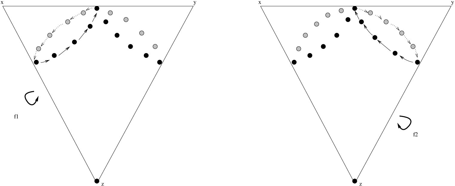
Let S0,m+2S_{0,m+2} be a genus 00 surface with m+2m+2 marked points (i.e. a marked sphere), and we recall an example of pseudo-Anosov ϕ∈Mod⁡(S0,m+2)\phi\in\mathrm{Mod}(S_{0,m+2}) in [HK06]. We view S0,m+2S_{0,m+2} as a sphere with s+1s+1 marked points XX circling an unmarked point xx and t+1t+1 marked points YY circling an unmarked point yy, and a single extra marked point zz. We can also draw this as a “turnover”, as in Figure 2. Note that |X∩Y|=1|X\cap Y|=1, |X|=s+1|X|=s+1, |Y|=t+1|Y|=t+1 and m=s+tm=s+t.

Refer to caption
Figure 2: Two way of viewing a marked sphere. Black dots are marked points and the shaded dots on the right are marked points at the back.

We define homeomorphisms αs\alpha_{s}, βt:S0,m+2→S0,m+2\beta_{t}:S_{0,m+2}\rightarrow S_{0,m+2} such that αs\alpha_{s} rotates the marked points of XX counterclockwise around xx and βt\beta_{t} rotates the marked points of YY clockwise around yy; see Figure 3. Define ϕs,t:=βt​αs\phi_{s,t}:=\beta_{t}\alpha_{s}.

Refer to caption
Figure 3: Homeomorphisms αs\alpha_{s} and βt\beta_{t}.

In [HK06], it is shown that ϕs,t\phi_{s,t} is pseudo-Anosov by checking it satisfies the criterion of [BH95]. We also note that from this one can check that xx, yy and zz are fixed points of a pseudo-Anosov representative of ϕs,t\phi_{s,t}. Moreover, for ss, t≥1t\geq 1 the dilatation of ϕs,t\phi_{s,t} equals the largest root of the polynomial

Ts,t​(x)\displaystyle T_{s,t}(x) =xt+1​(xs​(x−1)−2)+xs+1​(x−s​(x−1−1)−2)\displaystyle=x^{t+1}(x^{s}(x-1)-2)+x^{s+1}(x^{-s}(x^{-1}-1)-2)
=(x−1)​x(s+t+1)−2​(xs+1+xt+1)−(x−1).\displaystyle=(x-1)x^{(s+t+1)}-2(x^{s+1}+x^{t+1})-(x-1).

The dilatation is minimized when s=⌊m2⌋s=\lfloor\frac{m}{2}\rfloor and t=⌈m2⌉t=\lceil\frac{m}{2}\rceil. Let us define ϕ:=ϕ⌊m2⌋​,​⌈m2⌉\phi:=\phi_{\lfloor\frac{m}{2}\rfloor\text{,}\lceil\frac{m}{2}\rceil} and its dilatation is the largest root of the polynomial

Tm​(x)\displaystyle T_{m}(x) :=T⌊m2⌋​,​⌈m2⌉​(x)\displaystyle:=T_{\lfloor\frac{m}{2}\rfloor\text{,}\lceil\frac{m}{2}\rceil}(x)
=(x−1)​x(m+1)−2​(x⌊m2⌋+1+x⌈m2⌉+1)−(x−1).\displaystyle=(x-1)x^{(m+1)}-2\left(x^{\lfloor\frac{m}{2}\rfloor+1}+x^{\lceil\frac{m}{2}\rceil+1}\right)-(x-1).
Proposition 4.1.

If m≥5m\geq 5, then the largest real root of Tm​(x)T_{m}(x) is bounded above by m3mm^{\frac{3}{m}}.

Proof.

For all mm, we have Tm​(1)=−4T_{m}(1)=-4. It is sufficient to show that for all x≥m3mx\geq m^{\frac{3}{m}}, we have Tm​(x)>0T_{m}(x)>0. Dividing the inequality by x(m+1)x^{(m+1)}, it is equivalent to show

(x−1)+x−(m+1)>2​(x⌊m2⌋−m+x⌈m2⌉−m)+x−m.\displaystyle(x-1)+x^{-(m+1)}>2\left(x^{\lfloor\frac{m}{2}\rfloor-m}+x^{\lceil\frac{m}{2}\rceil-m}\right)+x^{-m}.

For m≥5m\geq 5, one can verify the following inequalities hold for all x≥m3mx\geq m^{\frac{3}{m}}

  1. 1.

    x−1>3​log⁡mm≥92​mx-1>\frac{3\log m}{m}\geq\frac{9}{2m},

  2. 2.

    x⌊m2⌋−m≤x⌈m2⌉−m≤1mx^{\lfloor\frac{m}{2}\rfloor-m}\leq x^{\lceil\frac{m}{2}\rceil-m}\leq\frac{1}{m},

  3. 3.

    x−m≤125​mx^{-m}\leq\frac{1}{25m}.

Therefore,

(x−1)+x−(m+1)\displaystyle(x-1)+x^{-(m+1)} >x−1>92​m>10125​m=2​(1m+1m)+125​m\displaystyle>x-1>\frac{9}{2m}>\frac{101}{25m}=2(\frac{1}{m}+\frac{1}{m})+\frac{1}{25m}
≥2​(x⌊m2⌋−m+x⌈m2⌉−m)+x−m.\displaystyle\geq 2\left(x^{\lfloor\frac{m}{2}\rfloor-m}+x^{\lceil\frac{m}{2}\rceil-m}\right)+x^{-m}.

∎

Remark.

Proposition 4.1 fails if we try to replace the bound with c1mc^{\frac{1}{m}} where cc is any constant.

Remark.

ϕs,t\phi_{s,t} is not the example which gives the best upper bound on l0,ml_{0,m} in [HK06]. In fact they show log⁡λ⁡(ϕs,t)\log\lambda(\phi_{s,t}) is strictly greater than l0,ml_{0,m} for m≥8m\geq 8, for all ss and tt.

Next, we take a cyclic branched cover S2,nS_{2,n} of S0,m+2S_{0,m+2} with branched points xx, yy, zz where n=5​(m+1)+1n=5(m+1)+1. See Figure 4. Define X~={marked points around ​x~}\widetilde{X}=\{\text{marked points around }\widetilde{x}\} and Y~={marked points around ​y~}\widetilde{Y}=\{\text{marked points around }\widetilde{y}\}, so we have |X~∩Y~|=5|\widetilde{X}\cap\widetilde{Y}|=5, |X~|=5​(s+1)|\widetilde{X}|=5(s+1) and |Y~|=5​(t+1)|\widetilde{Y}|=5(t+1).

Refer to caption
Figure 4: π\pi is the covering map. To form S2,nS_{2,n} from the decagon, identify the opposite sides. Then π\pi is the quotient by the group generated by rotation of an angle 2​π/52\pi/5.

We lift αs\alpha_{s}, βt\beta_{t} to S2,nS_{2,n} and call them αs~\widetilde{\alpha_{s}}, βt~\widetilde{\beta_{t}}, so that αs~\widetilde{\alpha_{s}} rotates the marked points of X~\widetilde{X} counterclockwise around x~\widetilde{x} and βt~\widetilde{\beta_{t}} rotates the marked points of Y~\widetilde{Y} clockwise around y~\widetilde{y}; see Figure 5. We define ψs,t:=βt~​αs~\psi_{s,t}:=\widetilde{\beta_{t}}\widetilde{\alpha_{s}}. It follows that ψs,t\psi_{s,t} is a lift of ϕs,t\phi_{s,t}, and so is pseudo-Anosov with λ⁡(ψs,t)=λ⁡(ϕs,t)\lambda(\psi_{s,t})=\lambda(\phi_{s,t}). An invariant train track for ψs,t\psi_{s,t} is obtained by lifting the one constructed in [HK06], and is shown in Figure 6 for s=t=3s=t=3.

Refer to caption
Figure 5: Homeomorphisms αs~\widetilde{\alpha_{s}} and βt~\widetilde{\beta_{t}}.
Refer to caption
Figure 6: A train track for ψ3,3\psi_{3,3}

Hence for n=5​(m+1)+1≥31n=5(m+1)+1\geq 31, we have constructed a pseudo-Anosov ψ=ψ⌊m2⌋​,​⌈m2⌉∈Mod⁡(S2,n)\psi=\psi_{\lfloor\frac{m}{2}\rfloor\text{,}\lceil\frac{m}{2}\rceil}\in\mathrm{Mod}(S_{2,n}) with λ⁡(ψ)=λ⁡(ϕ)≤m3m\lambda(\psi)=\lambda(\phi)\leq m^{\frac{3}{m}} which implies

log⁡λ⁡(ψ)≤3​log⁡mm=15​log⁡(n−6)−15​log⁡5n−6.\displaystyle\log\lambda(\psi)\leq\frac{3\log m}{m}=\frac{15\log(n-6)-15\log 5}{n-6}.

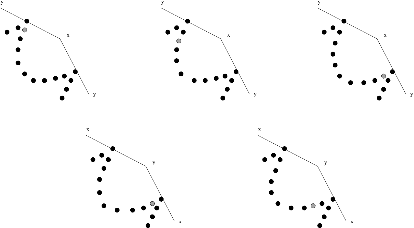
We will now extend ψ\psi so that nn can be an arbitrary number ≥31\geq 31. We add an extra marked point p1p_{1} on S2,nS_{2,n} between points in X~\widetilde{X} or Y~\widetilde{Y} except the places shown in Figure 7.

Refer to caption
Figure 7: We are not allowed to add p1p_{1} in the places indicated by a shaded point.

Without loss of generality we assume p1p_{1} is added in X~\widetilde{X} to obtain S2,n+1S_{2,n+1} and we define ψ1:=βt~​αs~′∈Mod⁡(S2,n+1)\psi_{1}:=\widetilde{\beta_{t}}\widetilde{\alpha_{s}}^{\prime}\in\mathrm{Mod}(S_{2,n+1}) where αs~′\widetilde{\alpha_{s}}^{\prime} is extended from αs~\widetilde{\alpha_{s}} in the obvious way; see Figure 8.

Refer to caption
Figure 8: The homeomorphism αs~′\widetilde{\alpha_{s}}^{\prime}. The figure on the right is a local picture near the added point p1p_{1}.

One can check that ψ1\psi_{1} is pseudo-Anosov via the techniques of [BH95]. An invariant train track for ψ1\psi_{1} is shown in Figure 9 and is obtained by modifying the invariant train track for ψ\psi shown in Figure 6.

Refer to caption
Figure 9: A train track for ψ1\psi_{1}. The figure on the bottom is a local picture.

Next, we will show λ⁡(ψ1)≤λ⁡(ψ)\lambda(\psi_{1})\leq\lambda(\psi). Let HH (respectively H1H_{1}) be the associated transition matrix of the train track map for ψ\psi (respectively ψ1\psi_{1}), and let Γ\Gamma (respectively Γ1\Gamma_{1}) be the induced directed graph as constructed in Section 2.2.

From the construction above (i.e. adding p1p_{1}), the directed graph Γ1\Gamma_{1} is obtained by adding a vertex on the edge going out from some vertex ii in Γ\Gamma (that is, subdividing the edge going out from ii) where ii has exactly one edge coming in and exactly one edge going out. This implies PΓ1​(i,k+1)=PΓ​(i,k)P_{\Gamma_{1}}(i,k+1)=P_{\Gamma}(i,k) and

PΓ1​(i,k+1)k+1≤PΓ1​(i,k+1)k=PΓ​(i,k)k\displaystyle\sqrt[k+1]{P_{\Gamma_{1}}(i,k+1)}\leq\sqrt[k]{P_{\Gamma_{1}}(i,k+1)}=\sqrt[k]{P_{\Gamma}(i,k)}

for all kk. Since HH and H1H_{1} are Perron-Frobenius matrices with Perron-Frobenius eigenvalues corresponding to the dilatations of ψ\psi and ψ1\psi_{1}, and Proposition 2.5 tells us μ⁡(H1)≤μ⁡(H)\mu(H_{1})\leq\mu(H), we have λ⁡(ψ1)=μ⁡(H1)\lambda(\psi_{1})=\mu(H_{1}) is no greater than λ⁡(ψ)=μ⁡(H)\lambda(\psi)=\mu(H).

We can obtain ψ2\psi_{2}, ψ3\psi_{3} and ψ4\psi_{4} by repeating the construction above of adding more marked points without increasing dilatations (i.e. λ⁡(ψc)≤λ⁡(ψ)\lambda(\psi_{c})\leq\lambda(\psi) for c=1,2,3,4c=1,2,3,4). Since log⁡mm≥log⁡(m+1)m+1\frac{\log m}{m}\geq\frac{\log(m+1)}{m+1}, we need not consider the cases with c≥5c\geq 5. Therefore, set f:S2,n→S2,nf:S_{2,n}\rightarrow S_{2,n} to be ψc\psi_{c}, where n=5​(m+1)+1+cn=5(m+1)+1+c with c<5c<5, and where ψ0=ψ\psi_{0}=\psi. For n≥31n\geq 31, we have

log⁡λ⁡(f)\displaystyle\log\lambda(f) ≤log⁡λ⁡(ψ)<3​log⁡mm<3​log⁡(n−115)(n−115),\displaystyle\leq\log\lambda(\psi)<\frac{3\log m}{m}<\frac{3\log\left(\frac{n-11}{5}\right)}{\left(\frac{n-11}{5}\right)},

where m=⌊n−65⌋m=\left\lfloor\frac{n-6}{5}\right\rfloor.

Theorem 4.2.

There exists κ2>0\kappa_{2}>0 such that l2,n<κ2​log⁡nnl_{2,n}<\frac{\kappa_{2}\log n}{n}, for all n≥3n\geq 3.

Proof.

From the discussion above, for n≥31n\geq 31,

l2,n<3​log⁡(n−115)(n−115)<κ2′​log⁡nn,\displaystyle l_{2,n}<\frac{3\log\left(\frac{n-11}{5}\right)}{\left(\frac{n-11}{5}\right)}<\frac{\kappa_{2}^{\prime}\log n}{n},

for some κ2′\kappa_{2}^{\prime}. For 3≤n≤303\leq n\leq 30, let κ2′′=max⁡{l2,3,l2,4,⋯,l2,30}\kappa_{2}^{\prime\prime}=\max\{l_{2,3},l_{2,4},\cdots,l_{2,30}\} then

l2,n≤κ2′′=(κ2′′​31log⁡31)​log⁡3131<(κ2′′​31log⁡31)​log⁡nn.\displaystyle l_{2,n}\leq\kappa_{2}^{\prime\prime}=\left(\kappa_{2}^{\prime\prime}\frac{31}{\log 31}\right)\frac{\log 31}{31}<\left(\kappa_{2}^{\prime\prime}\frac{31}{\log 31}\right)\frac{\log n}{n}.

Let κ2:=max⁡{κ2′,κ2′′​31log⁡31}\kappa_{2}:=\max\{\kappa_{2}^{\prime},\kappa_{2}^{\prime\prime}\frac{31}{\log 31}\}. ∎

4.2 Higher genus cases

We can generalize our construction and extend to any genus g>2g>2. For any fixed g>2g>2, we define ψ\psi to be a homeomorphism of Sg,nS_{g,n} in the same fashion with n=(2​g+1)​(m+1)+1n=(2g+1)(m+1)+1 by taking an appropriate branched cover over S0,m+2S_{0,m+2}, and we can again extend to arbitrary nn by adding cc extra marked points and constructing ψc\psi_{c}. Define f:Sg,n→Sg,nf:S_{g,n}\rightarrow S_{g,n} to be ψc\psi_{c} where n=(2​g+1)​(m+1)+1+cn=(2g+1)(m+1)+1+c. If n≥6​(2​g+1)+1n\geq 6(2g+1)+1, then

log⁡λ⁡(f)\displaystyle\log\lambda(f) <3​log⁡mm​, where ​m=⌊n−12​g+1⌋−1\displaystyle<\frac{3\log m}{m}\text{, where }m=\left\lfloor\frac{n-1}{2g+1}\right\rfloor-1
<3​log⁡(n−4​g−32​g+1)(n−4​g−32​g+1).\displaystyle<\frac{3\log\left(\frac{n-4g-3}{2g+1}\right)}{\left(\frac{n-4g-3}{2g+1}\right)}.
Theorem 4.3.

For any fixed g≥2g\geq 2, there exists κg>0\kappa_{g}>0 such that lg,n<κg​log⁡nnl_{g,n}<\frac{\kappa_{g}\log n}{n}, for all n≥3n\geq 3.

Proof.

This is similar to the proof of Theorem 4.2, where κg:=max⁡{κg′,κg′′​12​g+7log⁡(12​g+7)}\kappa_{g}:=\max\{\kappa_{g}^{\prime},\kappa_{g}^{\prime\prime}\frac{12g+7}{\log(12g+7)}\}. ∎

Proof of Theorem 1.1.

We only need to prove that the lower bounds on log⁡λ⁡(f)\log\lambda(f) of Theorem 3.3 are bounded below by log⁡nωg​n\frac{\log n}{\omega_{g}n} for some ωg\omega_{g} depending only on gg, then let cg=max⁡{κg,ωg}c_{g}=\max\{\kappa_{g},\omega_{g}\}. We use the monotone decreasing property of log⁡nn\frac{\log n}{n} for n≥3n\geq 3. Let

ωg′​(α):=α⁡(12​g−12)log⁡2​log⁡33≥α⁡(12​g−12)log⁡2​log⁡nn\displaystyle\omega^{\prime}_{g}(\alpha):=\frac{\alpha(12g-12)}{\log 2}\frac{\log 3}{3}\geq\frac{\alpha(12g-12)}{\log 2}\frac{\log n}{n}

and so

log⁡2α⁡(12​g−12)≥log⁡nωg′​(α)​n.\displaystyle\frac{\log 2}{\alpha(12g-12)}\geq\frac{\log n}{\omega^{\prime}_{g}(\alpha)n}.

For n≥g−1n\geq g-1,

log⁡(18​g+6​n−18)2​α​(18​g+6​n−18)≥log⁡24​n2​α​24​n>148​α​log⁡nn.\displaystyle\frac{\log(18g+6n-18)}{2\alpha(18g+6n-18)}\geq\frac{\log 24n}{2\alpha 24n}>\frac{1}{48\alpha}\frac{\log n}{n}.

For 3≤n<g−13\leq n<g-1,

log⁡(18​g+6​n−18)2​α​(18​g+6​n−18)>log⁡(24​(g−1))2​α​24​(g−1)≥log⁡(24​(g−1))2​α​24​(g−1)​3log⁡3​log⁡nn.\displaystyle\frac{\log(18g+6n-18)}{2\alpha(18g+6n-18)}>\frac{\log(24(g-1))}{2\alpha 24(g-1)}\geq\frac{\log(24(g-1))}{2\alpha 24(g-1)}\frac{3}{\log 3}\frac{\log n}{n}.

Let ωg:=max⁡{ωg′​(α),48​α,48​α​(g−1)​log⁡33​log⁡(24​(g−1))}\omega_{g}:=\max\{\omega^{\prime}_{g}(\alpha),48\alpha,\frac{48\alpha(g-1)\log 3}{3\log(24(g-1))}\}, where 0≤α≤Θ⁡(g)0\leq\alpha\leq\Theta(g). ∎

5 Appendix

We will construct a example to prove that l1,2​nl_{1,2n} has an upper bound of the same order as Penner’s lower bound in [Pen91], i.e. l1,2​n=O⁡(1n)l_{1,2n}=O(\frac{1}{n}). The construction is analogous to the one given by Penner for Sg,0S_{g,0} in [Pen91].

Let S1,2​nS_{1,2n} be a marked torus of 2​n2n marked points. Let aa and bb be essential simple closed curves as in Figure 10.

Refer to caption
Figure 10: Essential simple closed curves aa and bb on a marked torus.

Let Ta−1T_{a}^{-1} be the left Dehn twist along aa and TbT_{b} be the right Dehn twist along bb, then we define

f:=ρ∘Tb∘Ta−1∈Mod⁡(S1,2​n)\displaystyle f:=\rho\circ T_{b}\circ T_{a}^{-1}\in\mathrm{Mod}(S_{1,2n})

where ρ\rho rotates the torus clockwise by an angle of 2​π/n2\pi/n, so it sends each marked point to the one which is two to the right. As in [Pen88], fnf^{n} is shown to be pseudo-Anosov, and thus so is ff. Figure 11 shows a bigon track for fnf^{n}.

Refer to caption
Figure 11: A bigon track for fnf^{n}.

We obtain the transition matrix MnM^{n} associated to the train track map of fnf^{n} where MnM^{n} is an integral Perron-Frobenius matrix and the Perron-Frobenius eigenvalues μ⁡(Mn)\mu(M^{n}) is the dilatation λ⁡(fn)\lambda(f^{n}) of fnf^{n}. For n≥5n\geq 5,

Mn=(11010000⋯⋯000012010000⋯⋯001000110100⋯⋯000011130100⋯⋯000000001101⋯⋯000000111301⋯⋯000000000011⋯⋯000000001113⋯⋯000000000000⋯⋯000000000011⋯⋯000000000000⋯⋯0000⋮⋮⋮⋮⋮⋮⋮⋮⋯⋯⋮⋮⋮⋮00000000⋯⋯000000000000⋯⋯010000000000⋯⋯010000000000⋯⋯110100000000⋯⋯130112010000⋯⋯002112010000⋯⋯1123)2​n×2​n.\displaystyle M^{n}=\left(\begin{array}[]{cccccccccccccc}1&1&0&1&0&0&0&0&\cdots&\cdots&0&0&0&0\\ 1&2&0&1&0&0&0&0&\cdots&\cdots&0&0&1&0\\ 0&0&1&1&0&1&0&0&\cdots&\cdots&0&0&0&0\\ 1&1&1&3&0&1&0&0&\cdots&\cdots&0&0&0&0\\ 0&0&0&0&1&1&0&1&\cdots&\cdots&0&0&0&0\\ 0&0&1&1&1&3&0&1&\cdots&\cdots&0&0&0&0\\ 0&0&0&0&0&0&1&1&\cdots&\cdots&0&0&0&0\\ 0&0&0&0&1&1&1&3&\cdots&\cdots&0&0&0&0\\ 0&0&0&0&0&0&0&0&\cdots&\cdots&0&0&0&0\\ 0&0&0&0&0&0&1&1&\cdots&\cdots&0&0&0&0\\ 0&0&0&0&0&0&0&0&\cdots&\cdots&0&0&0&0\\ \vdots&\vdots&\vdots&\vdots&\vdots&\vdots&\vdots&\vdots&\cdots&\cdots&\vdots&\vdots&\vdots&\vdots\\ 0&0&0&0&0&0&0&0&\cdots&\cdots&0&0&0&0\\ 0&0&0&0&0&0&0&0&\cdots&\cdots&0&1&0&0\\ 0&0&0&0&0&0&0&0&\cdots&\cdots&0&1&0&0\\ 0&0&0&0&0&0&0&0&\cdots&\cdots&1&1&0&1\\ 0&0&0&0&0&0&0&0&\cdots&\cdots&1&3&0&1\\ 1&2&0&1&0&0&0&0&\cdots&\cdots&0&0&2&1\\ 1&2&0&1&0&0&0&0&\cdots&\cdots&1&1&2&3\\ \end{array}\right)_{2n\times 2n}.

Note that pairs of columns in the middle of the matrix shift down by 22 in succession. For n≥5n\geq 5, the greatest column sum of MnM^{n} is 99 and the greatest row sum of MnM^{n} is 1111. One can verify that both the greatest column sum and the greatest row sum are ≤11\leq 11 for 0<n≤40<n\leq 4. Therefore, for n≥1n\geq 1

11≥μ⁡(Mn)=λ⁡(fn)=(λ⁡(f))n\displaystyle 11\geq\mu(M^{n})=\lambda(f^{n})=(\lambda(f))^{n}
⇒l1,2​n≤log⁡λ⁡(f)≤log⁡11n.\displaystyle\Rightarrow l_{1,2n}\leq\log\lambda(f)\leq\frac{\log 11}{n}.

References

  • [Bau92] Max Bauer. An upper bound for the least dilatation. Trans. Amer. Math. Soc., 330(1):361–370, 1992.
  • [BH95] M. Bestvina and M. Handel. Train-tracks for surface homeomorphisms. Topology, 34(1):109–140, 1995.
  • [BT82] Raoul Bott and Loring W. Tu. Differential forms in algebraic topology, volume 82 of Graduate Texts in Mathematics. Springer-Verlag, New York, 1982.
  • [FLP91] A. Fathi, F. Laudenbach, and V. Poénaru. Travaux de Thurston sur les surfaces. Société Mathématique de France, Paris, 1991. Séminaire Orsay, Reprint of Travaux de Thurston sur les surfaces, Soc. Math. France, Paris, 1979 Astérisque No. 66-67 (1991).
  • [Gan59] F. R. Gantmacher. The theory of matrices. Vols. 1, 2. Translated by K. A. Hirsch. Chelsea Publishing Co., New York, 1959.
  • [GP74] Victor Guillemin and Alan Pollack. Differential topology. Prentice-Hall Inc., Englewood Cliffs, N.J., 1974.
  • [HK06] Eriko Hironaka and Eiko Kin. A family of pseudo-Anosov braids with small dilatation. Algebr. Geom. Topol., 6:699–738 (electronic), 2006.
  • [Iva88] N. V. Ivanov. Coefficients of expansion of pseudo-Anosov homeomorphisms. Zap. Nauchn. Sem. Leningrad. Otdel. Mat. Inst. Steklov. (LOMI), 167(Issled. Topol. 6):111–116, 191, 1988.
  • [Iva92] Nikolai V. Ivanov. Subgroups of Teichmüller modular groups, volume 115 of Translations of Mathematical Monographs. American Mathematical Society, Providence, RI, 1992. Translated from the Russian by E. J. F. Primrose and revised by the author.
  • [McM00] Curtis T. McMullen. Polynomial invariants for fibered 3-manifolds and Teichmüller geodesics for foliations. Ann. Sci. École Norm. Sup. (4), 33(4):519–560, 2000.
  • [Min06] Hiroyuki Minakawa. Examples of pseudo-Anosov homeomorphisms with small dilatations. J. Math. Sci. Univ. Tokyo, 13(2):95–111, 2006.
  • [Pen88] Robert C. Penner. A construction of pseudo-Anosov homeomorphisms. Trans. Amer. Math. Soc., 310(1):179–197, 1988.
  • [Pen91] R. C. Penner. Bounds on least dilatations. Proc. Amer. Math. Soc., 113(2):443–450, 1991.
  • [PH92] R. C. Penner and J. L. Harer. Combinatorics of train tracks, volume 125 of Annals of Mathematics Studies. Princeton University Press, Princeton, NJ, 1992.

Chia-yen Tsai:
Department of Mathematics, University of Illinois, Urbana-Champaign, IL 61801
ctsai6@math.uiuc.edu