Stochastic models and numerical algorithms
for a class of regulatory gene networks

Thomas Fournier Jean-Pierre Gabriel Christian Mazza Jerôme Pasquier
José Galbete and Nicolas Mermod ^†^†thanks: Department of Mathematics, University of Fribourg,Chemin du Musée 23,CH-1700 Fribourg, Switzerland, christian Mazza@unifr.ch^†^†thanks: Institute of Biotechnology, University of Lausanne, CH-1015 Lausanne, Switzerland, nicolas.mermod@unil.ch

February 2008

Regulatory gene networks contain generic modules, like those involving feedback loops, which are essential for the regulation of many biological functions [18]. We consider a class of self-regulated genes which are the building blocks of many regulatory gene networks, and study the steady-state distribution of the associated Gillespie algorithm by providing efficient numerical algorithms. We also study a regulatory gene network of interest in gene therapy, using mean-field models with time delays. Convergence of the related time-nonhomogenous Markov chain is established for a class of linear catalytic networks with feedback loops.

Keywords: Gillespie algorithm, gene network, self promoter, quasi-equilibrium, dimerization, mean field, time delay.

1 Introduction

Modeling of the regulation of all genes in a given cell is a tantalizing problem in biology and medicine (see, e.g. [18]). Recent developments allow rapid experimental determination of the expression of nearly all genes in a given biological setting, to an extent that in depth analysis and proper mathematical understanding of these vast arrays of data has become limiting. Qualitative models of regulatory networks, where particular genes code for proteins that activate or repress other genes, are being assembled, but models taking the stochastic and quantitative nature of gene regulation remain scarce, and they often rely on assumptions or simplifications that rest untested experimentally. Thus, it would be useful to build validated mathematical models of particular regulatory modules, as a first step towards constructing models of genome-wide gene expression.

Here, we consider a class of self-regulated genes, as depicted in Figure 1. This auto-regulated module is a very common building block of many gene networks, as it may form the basis of stochastic gene switches that contribute to biological decisions such as cell differentiation, and has been studied extensively in the literature in some special settings, as in [31], [21] or [23]. In a previous work, [11], we provided the exact steady-state distribution of the stochastic expression level of the autoregulated gene using the Gillespie algorithm in a general setting. We will present a direct version of the method and study more deeply this stationary distribution by providing efficient numerical algorithms. We will also consider a synthetic regulatory network acting as a genetic switch that was studied in living cells [22].

Refer to caption — Figure 1: The self-regulated gene

A self-regulated gene

The system is composed of a promoter and a gene, as schematized in Figure 1. As stated previously, one source of molecular noise is the random nature of the states taken by the promoter (on/off). Figure 1 shows protein monomers produced by the RNA polymerase during the transcription and translation processes. Protein monomers react quickly to form dimers: we assume a quasi-equilibrium where fast reactions equilibrate instantaneously. For a global amount of n proteins, the proportion of dimers at quasi-equilibrium is a well defined function of n. Dimers can bind to some sites near the promoter, and therefore enhance transcription, corresponding to a positive feedback loop. These binding events can be assumed to be fast with respect to events like protein formation. They are however included in some chain of events which ends with a state where the right positioning of the RNA polymerase is possible. This will correspond to the on state ${\cal O}_{1}$ . When these conditions are not satisfied, the promoter is off ${\cal O}_{0}$ . The rates of transitions between these two states are functions of the proportion of dimers, and therefore of n when the cell contains n proteins. These random events are usually modeled by supposing that the probability that the promoter switches from the off to on state in a small time interval of length $h\approx 0$ is of order g(n)h for n proteins, where the function g can be chosen according to the specificity of the setting. To be as general as possible, and to eventually allow negative feedback loops, we also assume that the probability of transition of the reverse reaction is given by some function $\kappa(n)$ . Basal activity is introduced by supposing that g(0) is positive, so that the required conditions for an eventual transcription event can be realized without protein dimers. The remaining involved chemical reactions are essentially protein monomers production and degradation, which are summarized in Figure 1. Transcription is stopped when the promoter is off, so that we assume that the probability $\mu_{0}h$ that a protein is created during a small time interval of length h vanishes, with $\mu_{0}=0$ . When the promoter is on, transcription is possible, and the probability that a transcription event occurs is of order $\mu_{1}h$ . Degradation of protein dimers is summarized by the rate $\nu(n)$ , for some function $\nu$ , which is usually linear as a function of $n$ . The time evolution of the state of this self regulated gene is described by a pair of time continuous stochastic process N(t) and Y(t), where N(t) gives the number of proteins present in the cell at time t and where Y(t) takes the values 0 and 1 corresponding to the off and on states of the promoter. The usual way of simulating N(t) and Y(t) proceeds by running the Gillespie algorithm (see e.g. [15], and [7]). The mean steady state expression level is thus obtained through Monte-Carlo experiments.

A regulatory network for efficient control of transgene expression

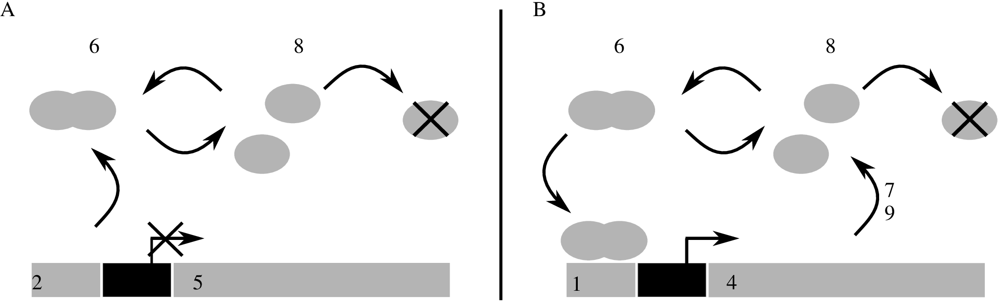
A more elaborate gene network consists of three genes. A first gene encodes a transcriptional repressor. Because this gene is expressed from an unregulated promoter, it mediates a stable number of repressor. This repressor binds to and inhibits the promoters of the two other genes, coding for a transactivator protein and for a quantifiable or a therapeutic protein, respectively (Figure 2A). The activity of the repressor is inhibited by doxycycline, a small antibiotic molecule that acts as a ligand of the repressor and thereby controls its activity. Addition of the antibiotic will inhibit the repressor and relieve repression, allowing low levels of expression of the regulated genes and synthesis of some transactivator protein. This, in turn, allows further activation of the two regulated genes, in a positive feedback loop (Figure 2B). When introduced in mammalian cells, this behaves as a signal amplifier and as a potent genetic switch, where the expression of a therapeutic gene can be controlled to vary from almost undetectable to very high levels in response to the addition of the antibiotic to the cells ([22], and [11]).

Results

Section 2 considers the Gillespie algorithm for simulating the time evolution of the number of proteins $N(t)$ and of the state of of the related promoter $Y(t)$ , by focusing on the associated steady state distribution $\pi$ . In a previous work [11], we gave an explicit formula for the steady-state associated to self-regulated genes, based on the embedded jump chain of the time continuous Markov process. Here we introduce a direct version dealing with the time continuous process. For concrete computation, we have to use a bounded state space with a total number of proteins that can not exceed a fixed but arbitrary integer $\Lambda$ . ALGORITHM I gives an efficient way of computing $\pi$ and a useful tightness argument to show that the sequence of steady-state distributions measures indexed by $\Lambda$ converges as $\Lambda\to\infty$ to the unique invariant distribution of the process defined on the unbounded state space ${\mathbb{N}}\times\{0,1\}$ . We also provide information on the variance of the gene product at steady state using generating functions and differential equations.

Section 3 proposes a mean field model with time delays, generalizing a model considered recently in this setting by [17], by including stochastic signals related to promoters. The feedback rates $g(N(t))$ and $\kappa(N(t))$ are replaced by $g({\mathbb{E}}(N(t-\theta)))$ and $\kappa({\mathbb{E}}(N(t-\theta)))$ . In [11], we studied the regulatory gene network in living cells; the obtained experimental results were in good concordance with the model’s predictions. The related functions $E(t)={\mathbb{E}}(N(t))$ and $G(t)=P(Y(t)=1)$ sastisfy the time delayed differential system

\frac{dE}{dt}=\mu G(t)-\nu E(t),\ \ \ \frac{dG}{dt}=g(E(t-\theta))(1-G(t))-\kappa(E(t-\theta))G(t),

which can be deduced from the chemical master equation, see Section 5. As it is well known, this kind of differential systems can possess oscillating or periodic solutions, see e.g. [5]. We show that there is a globally asymptotically stable equilibrium point when $g$ is such that $g(n)/n$ is decreasing as function of $n$ and $\kappa(n)\equiv\kappa$ . We next provide ALGORITHM II for computing the steady state variance. Section 4 deals with two time scales stochastic simulations and processes evolving at quasi-equilibrium. We also consider a generic dimerization process which occurs in most biochemical reaction networks, and provide an efficient ALGORITHM III for computing the first two moments of the related steady state distribution, which are then used when dealing with systems evolving at quasi-equilibrium. Finally, Section 5 focus on the regulatory network; we model extrinsic and intrinsic noise using a mean-field model, which permits to study the fluctuations of the variance of the number of therapeutic proteins as function of the number of doxycycline molecules.

2 Mathematical models related to the self-regulated gene

In what follows, we consider the time continuous Markov chain known as the Gillespie algorithm for simulating the self regulated gene with arbitraries feedback mechanisms, and give precise formulas for the related steady state distribution $\pi$ . We shall see in Section 5.4 a semi-stochastic or mean field model for the therapeutic network. The related steady state distribution is obtained as the product of steady state distributions of sub modules corresponding to self regulated genes. A complete understanding of basic modules like the self regulated gene is thus fundamental for understanding the global network, see e.g. [18] and Section 5.4. For more details on the model, see [11].

The module is composed of a promoter and a gene. Its time evolution is given by the following set of chemical reactions:

{\cal P}{\overset{\nu(n)}{\longrightarrow}}\emptyset,\ \ \emptyset{\overset{\mu_{l}}{\longrightarrow}}{\cal P},\ l=0,1,

represents degradation of gene product when they are $n$ molecules, here proteins ( ${\cal P}$ ), and protein production, where $l=0$ means that the promoter is off: no transcription factor (a complex composed of gene product) is bound to some operator sites near the promoter, so that the RNA polymerase can’t bind well in the neighborhood of the basal promoter. We assume here that the transcription rate $\mu_{0}$ is such that $\mu_{0}\approx 0$ . When $l=1$ , meaning that the promoter is on, transcription occurs at a rate $\mu_{1}=\mu$ . The fluctuations of the state of the promoter are described by the following reaction

{\cal O}_{0}\underset{\kappa(n)}{\overset{g(n)}{\longleftrightarrow}}{\cal O}_{1},

where ${\cal O}_{l}$ , $l\in\{0,1\}$ , indicates the state of the promoter. The transitions from the on to off states ${\cal O}_{1}{\overset{\kappa(n)}{\longrightarrow}}{\cal O}_{0}$ occur at rate $\kappa(n)$ , and the reverse reactions at rate $g(n)$ . Here $g$ and $\kappa$ are two functions of the number of proteins modeling positive and negative feedback loops.

Basal activity is introduced at the level of the reaction ${\cal O}_{0}{\overset{g(n)}{\longrightarrow}}{\cal O}_{1}$ , by supposing that $g>0$ . The Gillespie algorithm for simulating the above chemical reactions is a bivariate Markov process $\eta(t)$ $=(N(t),Y(t))$ , with $N(t)\leqslant\Lambda$ and $Y(t)=0,1$ , where $N(t)$ denotes the number of proteins present in the cell at time $t$ , and $Y(t)$ represents the state of the operator. The time evolution of $Y(t)$ is coupled to that of $N(t)$ to model auto-regulation, using functions $g$ and $\kappa$ . For small time interval $(t,t+h)$ , $h\approx 0$ , the probability that the operator switches from the off to the on state is of order $g(N(t))h$ .

Let $p_{n}^{0}(t)=P(N(t)=n,Y(t)=0)$ and $p_{n}^{1}(t)=P(N(t)=n,Y(t)=1)$ give the probability of having $n$ proteins at time $t$ when the states of the promoter are ${\mathcal{O}}_{0}$ and ${\mathcal{O}}_{1}$ , respectively. We assume here that $0\leqslant n\leqslant\Lambda$ for some fixed but arbitrary integer $\Lambda$ . The related Gillespie algorithm is given as a time-continuous Markov chain $\eta(t)=(N(t),Y(t))$ (see e.g. [14]), where $N(t)\in\{0,1,\cdots,\Lambda\}$ and $Y(t)\in\{0,1\}$ , with transition rates given by

P((n,y),(n+1,y))=\mu_{y},\ P((n,y),(n-1,y))=\nu(n),

P((n,y),(n,1-y))=\kappa(n)\hbox{ when }y=1,\hbox{ and },

P((n,y),(n,1-y))=g(n)\hbox{ when }y=0.

The chemical master equation associated to the reaction scheme is then given by

\frac{{\rm d}p_{n}^{s}(t)}{{\rm d}t}=\mu_{s}(p_{n-1}^{s}(t)-p_{n}^{s}(t))+\nu(n+1)p_{n+1}^{s}(t)-\nu(n)p_{n}^{s}(t)

(2.1)

+(-1)^{s}(\kappa(n)p_{n}^{1}(t)-g(n)p_{n}^{0}(t)),

where $s\in\{0,1\}$ , see e.g. [23].

The steady-state distribution $\pi$ associated with (2.1) is obtained by letting $t\to\infty$ : $\pi$ is defined as

\pi_{n}(0)=\lim_{t\to\infty}p_{n}^{0}(t)\hbox{ and }\pi_{n}(1)=\lim_{t\to\infty}p_{n}^{1}(t),

and solves the linear system obtained from (2.1) by imposing ${\rm d}p_{n}^{s}/{\rm d}t=0$ :

0=\mu_{s}(\pi_{n-1}(s)-\pi_{n}(s))+\nu(n+1)\pi_{n+1}(s)-\nu(n)\pi_{n}(s)

+(-1)^{s}(\kappa(n)\pi_{n}(1)-g(n)\pi_{n}(0)),\ s=0,\ 1.

$\pi_{n}(0)$ is the probability to find $n$ proteins and that the promoter is off; $\pi_{n}(1)$ is defined similarly but for the on state. The probability of observing $n$ proteins at equilibrium is just $\pi_{n}(0)+\pi_{n}(1)$ .

In what follows, we derive the steady state distribution $\pi$ . This probability measure is used in the mean-field delayed model of Section 3 and in Section 5 for the study of the network.

2.1 Computing the steady-state

In this Section, we assume that $\mu_{0}=0$ , and that $\mu_{1}=\mu$ , where an explicit formula for the steady-state is available. The degradation propensity function $\nu(n)$ and the feedbacks $\kappa(n)$ and $g(n)$ are arbitrary positive functions.

The method of generating functions can be used in some particuliar special cases to compute the invariant measure, see [31] for the simple case whitout feedback with $\nu(n)=\nu\cdot n$ , $\kappa(n)\equiv\kappa$ and $g(n)\equiv g$ , or [21] for the case with linear negative feedback $\nu(n)=\nu\cdot n$ , $\kappa(n)\equiv\kappa\cdot n$ and $g(n)\equiv g$ . Although this method provides a powerful tool for analytic description, the method of generating functions is very particular in the sense that a little change in the form of one of the feedback propensity function can induce major changes in the generating function, and for each particular propensity function one has to derive the whole set of equations anew. Furthermore, an explicit form for the generating function can only be found when the feedback propensity functions are simple, either constant or linear in the protein numbers. In practice, the feedback propensity functions are related to the number of sites in the promoter on which the proteins bind, either directly in monomer form or in more complicated bound forms like dimers or higher order polymers, see [10].

In [11], we presented a general formula for the steady-state for arbitrary degradation and feedback propensity functions. The method relies on the asymptotic behaviour of the jump matrix of the embedded discrete jump chain. We provide here a direct version of this method allowing to compute the invariant distribution of the time continuous Markov process directly. We recall that we consider a bounded total number of protein $N(t)\leq\Lambda$ , a restriction that is biologically meaningful due to the finite volume of a cell but that is mainly supposed for technical reasons since the formula is recursive and we have to find a starting point $(\pi_{\Lambda}(0),\pi_{\Lambda}(1))$ to begin with. However, the condition is not restrictive and we show in Theorem 2 that the sequence of steady-state distributions indexed by the boundary $\Lambda$ converges weakly to the unique invariant distribution of the unbounded process on ${\mathbb{N}}\times\{0,1\}$ .

Let us define the transfer matrices

\alpha_{n}=\frac{\nu(n+1)}{\mu}\left[\begin{array}[]{cc}\frac{\kappa(n)+\mu}{g(n)+\nu(n)}&1\\ \frac{\kappa(n)}{g(n)+\nu(n)}&1\end{array}\right],\ 0<n<\Lambda,\quad\alpha_{0}=\frac{\nu(1)}{\mu}\left[\begin{array}[]{cc}\frac{\kappa(0)+\mu}{g(0)}&1\\ \frac{\kappa(0)}{g(0)}&1\end{array}\right],

and the vector $w_{\Lambda}=(\kappa(\Lambda),g(\Lambda)+\nu(\Lambda))$ .

Theorem 1

For $0\leq n\leq\Lambda$ , the invariant distribution

\pi_{n}=(\pi_{n}(0),\pi_{n}(1))=\lim_{t\to\infty}\left(P((N(t),Y(t))=(n,0)),P((N(t),Y(t))=(n,1))\right)

of the time-continuous Markov process $\{\eta(t)\}_{t>0}$ on the strip $\{0,1,\dots,\Lambda\}\times\{0,1\}$ is given by

\pi_{n}=\frac{w_{\Lambda}\alpha_{\Lambda-1}\alpha_{\Lambda-2}\cdots\alpha_{n}}{Z_{\Lambda}}\;\text{ for }\;0\leq n<\Lambda,\;\text{ and }\;\pi_{\Lambda}=\frac{w_{\Lambda}}{Z_{\Lambda}},

with the normalization constant

\displaystyle Z_{\Lambda}=w_{\Lambda}\cdot(1,1)^{T}+\sum_{j=0}^{\Lambda-1}w_{\Lambda}\alpha_{\Lambda-1}\alpha_{\Lambda-2}\cdots\alpha_{j}\cdot(1,1)^{T}.

Proof : At equilibrium, equations 2.1 reads

	$\displaystyle 0=$	$\displaystyle\pi_{0}R_{0}+\pi_{1}D_{1},$
	$\displaystyle 0=$	$\displaystyle\pi_{n-1}U+\pi_{n}R_{n}+\pi_{n+1}D_{n+1},\quad 0<n<\Lambda,$
	$\displaystyle 0=$	$\displaystyle\pi_{\Lambda-1}U+\pi_{\Lambda}R_{\Lambda}.$

with the $2\times 2$ matrices $U=\left[\begin{array}[]{cc}0&0\\ 0&\mu\end{array}\right],$ $D_{n}=\left[\begin{array}[]{cc}\nu(n)&0\\ 0&\nu(n)\end{array}\right]$ and

R_{n}=\left[\begin{array}[]{cc}-(g(n)+\nu(n))&g(n)\\ \kappa(n)&-(\kappa(n)+\nu(n)+\mu)\end{array}\right]

for $1\leq n\leq\Lambda-1,$ and the boundaries $R_{0}=\left[\begin{array}[]{cc}-g(0)&g(0)\\ \kappa(0)&-(\kappa(0)+\mu)\end{array}\right],$

D_{\Lambda}=\left[\begin{array}[]{cc}\nu(\Lambda)&0\\ 0&\nu(\Lambda)\end{array}\right]\text{ and }R_{\Lambda}=\left[\begin{array}[]{cc}-(g(\Lambda)+\nu(\Lambda))&g(\Lambda)\\ \kappa(\Lambda)&-(\kappa(\Lambda)+\nu(\Lambda))\end{array}\right].

Simple linear algebra shows that the above defined matrices $\alpha_{n}$ , $0\leq n<\Lambda$ , satisfy the relation $\pi_{n}=\pi_{n+1}\alpha_{n}$ . Indeed one only has to check that for $0<n<\Lambda$ , the $2\times 2$ matrices $\alpha_{n-1}U+R_{n}$ are invertible and that the matrices $\alpha_{n}$ solve the matrix continuous fraction

	$\displaystyle\alpha_{0}=$	$\displaystyle-D_{1}R_{0}^{-1},$
	$\displaystyle\alpha_{n}=$	$\displaystyle-D_{n+1}(\alpha_{n-1}U+R_{n})^{-1},\quad 0<n<\Lambda.$

$\square$

The formula given in Theorem 1 must be used with care numerically since, when $\Lambda$ is large, both the numerator and denominator rapidly diverge. It can be improved with the following normalization algorithm, that is exactly the same as the one used for the embedded jump chain in [11]. Let ${\mathbb{R}}_{\geq 0}^{2}:=\{w=(w_{1},w_{2}),w_{1},w_{2}\in{\mathbb{R}}_{\geq 0}\}$ with the $1$ -norm $\|w\|:=w\cdot(1,1)^{T}$ .

ALGORITHM I

(STEP 1): Define $\tilde{v}_{n}$ for $n=\Lambda-1$ to $0$ as

\tilde{v}_{\Lambda}:=\frac{w_{\Lambda}}{\|w_{\Lambda}\|},\quad\text{and}\quad\tilde{v}_{n}:=\frac{\tilde{v}_{n+1}\alpha_{n}}{\|\tilde{v}_{n+1}\alpha_{n}\|}.

(STEP 2): Given the $\tilde{v}_{n}$ , define $v_{0}=\tilde{v}_{0}$ and, for $n=1$ to $\Lambda$ , set

v_{n}:=\frac{\tilde{v}_{n}}{\|\tilde{v}_{n}\alpha_{n-1}\|\cdot\|\tilde{v}_{n-1}\alpha_{n-2}\|\cdots\|\tilde{v}_{1}\alpha_{0}\|}.

(STEP 3): Compute the steady-state distribution as

\pi_{n}=\frac{v_{n}}{V_{\Lambda}},\qquad\text{ where }\quad V_{\Lambda}:=\sum_{i=0}^{\Lambda}v_{i}\cdot{\bf 1}.

It immediately results from their definition that the $\tilde{v}_{n}$ and $v_{n}$ satisfy $\|\tilde{v}_{n}\|=1$ ,

v_{n}=\frac{\tilde{v}_{\Lambda}\alpha_{\Lambda-1}\alpha_{\Lambda-2}\cdots\alpha_{n}}{\|\tilde{v}_{\Lambda}\alpha_{\Lambda-1}\|\cdot\|\tilde{v}_{\Lambda-1}\alpha_{\Lambda-2}\|\cdots\|\tilde{v}_{n+1}\alpha_{n}\|\cdot\|\tilde{v}_{n}\alpha_{n-1}\|\cdots\|\tilde{v}_{1}\alpha_{0}\|},

the denominator of the above expression is independent of $n$ and $\tilde{v}_{\Lambda}$ is proportional to $w_{\Lambda}$ . Hence $v_{n}$ is proportional to the invariant measure $\pi_{n}$ , and (STEP 3) of the algorithm effectively compute the actual steady-state distribution.

Proposition 1 below provides conditions under which the normalization constant $V_{\Lambda}$ remains bounded as $\Lambda$ is large. The function $\nu(n)$ gives the monomer degradation rates for $n$ proteins, and is assumed to be increasing with $\nu(0)=0$ , and strictly positive for $n\geq 1$ . Usually, $\nu(n)$ is taken to be a constant times $n$ , here we assume the less restrictive condition that $\displaystyle\inf\limits_{n\geq 1}\nu(n)/n$ is stricly positive to allow situations where for example proteins that are present as chemical complexes (dimer, trimer,…) can not be degradated, or situations where $\nu(n)/n\to\infty$ as $n\to\infty$ .

Lemma 1

If $\displaystyle\inf\limits_{n\geq 1}\nu(n)/n$ is stricly positive, there exists a constant $k>0$ depending only on $\mu,\,\nu,\,\kappa,\,g$ (and not on $\Lambda$ ) such that for all $n\geq 1$ , $\|\tilde{v}_{n}\alpha_{n-1}\|\geq nk.$

Proof: Each $\tilde{v}_{j}$ lies in the line segment $S\subset{\mathbb{R}}^{2}$ between the points $(0,1)$ and $(1,0)$ and depends on $\Lambda$ . To break this dependence, we prove the results for an arbitrary vector $v=(t,1-t)\in S$ , $t\in[0,1]$ .

v\alpha_{n}=\frac{\nu(n)}{\mu}(\star,t+(1-t))=\frac{\nu(n)}{\mu}(\star,1),

with $\star>0$ for all $n$ . Hence, uniformly in $S$ ,

\frac{\|v\alpha_{n}\|}{n}\geq\frac{\nu(n)}{n\mu}\geq\inf\limits_{n\geq 1}\frac{\nu(n)}{n\mu}=:k>0.

$\square$

With Lemma 1 we can give bounds uniformly in $\Lambda$ :

Proposition 1

Assume that $\displaystyle\inf\limits_{n\geq 1}\nu(n)/n$ is stricly positive. There exists $M>0$ , depending only on $\mu,\,\nu,\,\kappa,\,g$ (and not on $\Lambda$ ), such that

\displaystyle 1\leq V_{\Lambda}=\sum_{n=0}^{\Lambda}\|v_{n}\|\leq M.

Proof : Notice that $\|v_{0}\|=\|\tilde{v}_{0}\|=1$ . The $1$ -norm of $v_{n}$ is

\|v_{n}\|=\frac{\|\tilde{v}_{n}\|}{\|\tilde{v}_{n}\alpha_{n-1}\|\cdots\|\tilde{v}_{1}\alpha_{0}\|}=\frac{1}{\|\tilde{v}_{n}\alpha_{n-1}\|\cdots\|\tilde{v}_{1}\alpha_{0}\|}

and with Lemma 1

V_{\Lambda}=1+\sum_{n=1}^{\Lambda}\|v_{n}\|\leq 1+\sum_{n=1}^{\infty}\frac{k^{-n}}{n!}=e^{1/k}=:M.

The first aim of lemma 1 is to show that the preceding algorithm is efficient. But this lemma can also be used to demonstrate that the steady-state distribution of the continuous-time process $\eta(t)$ converges when $\Lambda\to\infty$ . Moreover, we can show that this limiting distribution is the invariant distribution of the process on the unbounded strip.
It is necessary to adapt our notations in order to show the dependency in $\Lambda$ . Henceforth, we will write $\pi_{n}^{(\Lambda)}$ and $v_{n}^{(\Lambda)}$ instead of $\pi_{n}$ and $v_{n}$ .
Until now, we have considered a finite state-space by fixing a maximum number $\Lambda$ of proteins. It is always easier to deal with finite Markov chains, but the main reason is because our algorithm to compute the invariant measure works in this case. Even if this model is realistic (an organism cannot contain an infinite number of proteins), it is interesting to show that the steady-state does not depend asymptotically on this maximum number $\Lambda$ of proteins. In other words, we want to show that under a sufficient condition, the invariant measure converges in $\Lambda$ . We define $\pi^{(\Lambda)}=(\pi_{n}^{(\Lambda)})_{0\leq n\leq\Lambda}$ and consider the familiy of probalility measures $\Pi=(\pi^{(\Lambda)})_{\Lambda\in{\mathbb{N}}}$ embedded in ${\mathbb{N}}\times\{0,1\}$ .

Theorem 2

The sequence of invariant measures $\pi^{(\Lambda)}$ converges weakly as $\Lambda\to\infty$ to the invariant distribution of the process defined on the unbounded strip.

Proof: A sequence $\{P_{n}\}$ of probability distributions on a countable and discrete state space $E$ converges to the probability distribution $P$ on $E$ if and only if each of its subsequences $\{P_{n^{\prime}}\}$ contains a further subsequence $\{P_{n^{\prime\prime}}\}$ that converges to $P$ . A family $\Pi$ of probability distributions on $E$ is called relatively compact if every sequence of elements of $\Pi$ contains a convergent subsequence (to a probability distribution on $E$ ), and tight if for every positive $\epsilon$ there exists a compact set $K$ such that $P(K)>1-\epsilon$ for all $P$ in $\Pi$ . Tightness implies relative compactness, see e.g. [4].
We first show that the family of probalility distributions $\Pi=(\pi^{(\Lambda)})_{\Lambda\in{\mathbb{N}}}$ is tight. Lemma 1 implies that there exists $k$ not depending on $\Lambda$ such that

\|v_{n}^{(\Lambda)}\|\leq\frac{1}{n!\,k^{n}},\quad n\geq 1.

Since $V_{\Lambda}\geq 1$ , we have also

\|\pi_{n}^{(\Lambda)}\|=\frac{\|v_{n}^{(\Lambda)}\|}{V_{\Lambda}}\leq\frac{1}{n!\,k^{n}},\quad n\geq 1.

Hence, for all $\epsilon>0$ there exists $M_{\epsilon}$ (not depending on $\Lambda$ ) such that

\sum_{j=M_{\epsilon}}^{\infty}\|\pi_{j}^{(\Lambda)}\|\leq\sum_{j=M_{\epsilon}}^{\infty}\frac{1}{j!\,k^{j}}<\epsilon.

Consequently, $\Pi$ is relatively compact and there exists a convergent subsequence $(\pi^{(\Lambda_{k})})_{k\in{\mathbb{N}}}$ of $\Pi$ . Define $\pi^{(\infty)}=\lim_{k\to\infty}\pi^{(\Lambda_{k})}$ . We check now that $\pi^{(\infty)}$ is the invariant distribution of the continuous-time process defined on the unbounded strip. For each $n\in{\mathbb{N}}$ we have

	$\displaystyle\pi_{n}^{(\infty)}$	$\displaystyle=\lim_{k\to\infty}\pi_{n}^{(\Lambda_{k})}$
		$\displaystyle=\lim_{k\to\infty}(\pi_{n+1}^{(\Lambda_{k})}\,D_{n+1}+\pi_{n}^{(\Lambda_{k})}\,R_{n}+\pi_{n-1}^{(\Lambda_{k})}\,U)$
		$\displaystyle=\pi_{n+1}^{(\infty)}\,D_{n+1}+\pi_{n}^{(\infty)}\,R_{n}+\pi_{n-1}^{(\infty)}\,U.$

This shows that $\pi^{(\infty)}$ is indeed an invariant distribution of the limit chain. In fact, what preceded is also valid for any converging subsequence. Besides, the invariant distribution is unique because the process is irreducible. Thus, we can conclude that $\pi^{(\Lambda)}$ converges as $\Lambda\to\infty$ to $\pi^{(\infty)}$ which is the invariant distribution of the process defined on the unbounded strip. $\hfill\square$

2.2 The method of generating functions for the mean and variance

We consider the problem of computing the mean and variance of the gene product $N(t)$ at steady-state, that is when $t$ is large, using generating functions. As discussed in Section 2.1, generating functions allows in some simple cases to compute the steady-state distribution, see e. g. [31] or [21], with simple feedback functions. Here we show that even when the feedbacks are arbitrary, the method can be used to gain insight in the relations between variance, mean and probability to be ON. To avoid boundary conditions, we suppose here that the number of protein is arbitrary ( $\Lambda=\infty$ ), and the only asumption concerning the propensity functions is that $\nu(n)=\nu\ n$ , i. e. degradation is directly proportional to the number of proteins, while $\kappa(n)$ and $g(n)$ are arbitrary positive functions and $\mu_{0}$ is not necessarily $0$ .

Let $\pi_{n}(y)=\lim\limits_{t\to\infty}P(N(t)=n,Y(t)=y)$ and

\alpha(z)=\sum_{n\geqslant 0}\pi_{n}(1)z^{n},\qquad\qquad\beta(z)=\sum_{n\geqslant 0}\pi_{n}(0)z^{n},

be the partial generating functions related to the steady-state, and

R(z):=\sum_{n\geqslant 0}(\pi_{n}(1)\kappa(n)-\pi_{n}(0)g(n))z^{n}.

From the master equation (2.1) at equilibrium, we deduce

0=-R(z)+\mu_{1}(z-1)\alpha(z)+\nu(1-z)\frac{d\alpha(z)}{dz},\hbox{ and }0=+R(z)+\mu_{0}(z-1)\beta(z)+\nu(1-z)\frac{d\beta(z)}{dz}.

Adding these two relations and assuming that $z\neq 1$ gives

\frac{d\alpha(z)}{dz}+\frac{d\beta(z)}{dz}=\frac{\mu_{1}\alpha(z)+\mu_{0}\beta(z)}{\nu}.

This shows that the following general relations hold:

{\mathbb{E}}(N(\infty))=\frac{\mu_{1}}{\nu}P(Y(\infty)=1)+\frac{\mu_{0}}{\nu}P(Y(\infty)=0),

{\rm Var}(N(\infty))=\frac{\mu_{1}}{\nu}\frac{d\alpha(z)}{dz}|_{z=1}+\frac{\mu_{0}}{\nu}\frac{d\beta(z)}{dz}|_{z=1}+{\mathbb{E}}(N(\infty))(1-{\mathbb{E}}(N(\infty))),

where we recall that

\alpha(1)=P(Y(\infty)=1),\ \frac{d\alpha(z)}{dz}|_{z=1}={\mathbb{E}}(N(\infty)Y(\infty))\hbox{ and }\frac{d\beta(z)}{dz}|_{z=1}={\mathbb{E}}(N(\infty)(1-Y(\infty))).

These formulas make sense since, when the promoter is on (resp. off), the process evolves as a birth and death process with birth rate $\mu_{1}$ (resp. $\mu_{0}$ ) and death rate $\nu n$ , and has a Poisson distribution of parameter $\mu_{1}/\nu$ (resp. $\mu_{0}/\nu$ ) as a stationary distribution, of mean and the variance given by $\mu_{1}/\nu$ (resp. $\mu_{0}/\nu$ ). The last term is related to promoter fluctuations, see the following Example.

Example 1

Assume that $g(n)\equiv g$ and $\kappa(n)\equiv\kappa$ . Let $F(t)=\sum_{n\geqslant 0}nP(N(t)=n,Y(t)=1)$ . The master equation yields

\frac{dF(t)}{dt}=gE(t)+\mu_{1}G(t)-F(t)(g+\kappa+\nu),

\frac{dE(t)}{dt}=\mu_{1}G(t)+\mu_{0}(1-G(t))-\nu E(t),

where $E(t)={\mathbb{E}}(N(t))$ . Using the differential relation $dG(t)/dt=g(1-G(t))-\kappa G$ , one gets that

G(\infty)=\frac{g}{g+\kappa}.

Notice that $G(\infty)$ is related to the stationary law of the $0/1$ Markov chain given by the transition rates $p(0,1)=g$ and $p(1,0)=\kappa$ , which models the fluctuations of the state of the promoter. Then

	$\displaystyle{\rm Var}(N(\infty))$	$\displaystyle=$	$\displaystyle\frac{d^{2}\alpha(z)}{d^{2}z}\|_{z=1}+\frac{d^{2}\beta(z)}{d^{2}z}\|_{z=1}+E(\infty)-E(\infty)^{2}$
		$\displaystyle=$	$\displaystyle\frac{\mu_{1}}{\nu}F(\infty)+\frac{\mu_{0}}{\nu}H(\infty)+E(\infty)-E(\infty)^{2},$

where we set $H(t)=E(t)-F(t)$ . It follows that

{\rm Var}(N(\infty))=\frac{\mu_{1}}{\nu}G(\infty)+\frac{\mu_{0}}{\nu}(1-G(\infty))+\frac{\mu_{1}}{\nu}F(\infty)+\frac{\mu_{0}}{\nu}H(\infty)-E(\infty)^{2}.

We finally obtain, after some algebra,

{\rm Var}(N(\infty))=\frac{\mu_{1}}{\nu}G(\infty)+\frac{\mu_{0}}{\nu}(1-G(\infty))+\frac{\tau_{2}}{\tau_{1}+\tau_{2}}\frac{(\mu_{1}-\mu_{0})^{2}}{\nu^{2}}{\rm Var}(Y(\infty)),

where the characteristic times $\tau_{1}$ and $\tau_{2}$ are defined by

\tau_{1}=\frac{1}{\nu}\hbox{ and }\tau_{2}=\frac{1}{g+\kappa}.

The interpretation of this formula is obtained by observing that, when the promoter is on with probability $G(\infty)$ , the process evolves as a birth and death process with steady state distribution given by a Poisson distribution of parameter $\mu_{1}/\nu$ . The interpretation of the second term is similar. The third term corresponds to the variance of a Bernoulli random variable (on/off) multiplied by a factor accounting for characteristic times related to protein degradation and promoter fluctuation. When $\mu_{0}=0$ , the coefficient of variation can be then given as

CV^{2}_{N}=\frac{{\rm Var}(N(\infty))}{{\mathbb{E}}(N(\infty))^{2}}=\frac{1}{{\mathbb{E}}(N(\infty))}+\frac{\tau_{2}}{\tau_{1}+\tau_{2}}\frac{{\rm Var}(Y(\infty))}{{\mathbb{E}}(Y(\infty))^{2}},

as given in [30]. The above relations yield moreover that

CV^{2}_{N}=\frac{g+\kappa}{\rho g}+\frac{\nu\kappa}{g(g+\nu+\kappa)},

where $\rho=\mu_{1}/\nu$ , and it follows that $CV^{2}_{N}$ is decreasing as a function of $g$ and increasing as a function of $\kappa$ .

3 Mean-field models

Most mathematical works on gene networks, like [13], consider networks with linear transition rates in which the state space of each chemical species equals ${\mathbb{N}}$ . Results on networks involving catalytic transitions rates are very scarce. [24], also focus on such models but allow time dependent transition rates. In this situation, one gets interesting linear differential equations for the first and second moments, and for covariance functions. When some state space is finite, boundary effects transform the equations which become more involved.

The model for the self-regulated gene defined in Section 2 is similar to a mathematical model for an epidemic of schistosomiasis provided by [25] and [26]. In their model, the authors consider a similar Markov chain, where they replace every external random variables in the transitions probabilities by functions of their expected values. This means for example that the transition rate $P((n,y),(n+1,y))=y\mu$ is replaced by $P((n,y),(n+1,y))={\mathbb{E}}(Y(t))\mu$ , and $P((n,y),(n,1-y))$ by $\kappa({\mathbb{E}}(N(t)))y+g({\mathbb{E}}(N(t)))(1-y)$ , since for this last transition, the external random variable coresponding to this transition is $N(t)$ . One gets a time-nonhomogeneous Markov chain. One can show that the pair $({\mathbb{E}}(N(t)),{\mathbb{E}}(Y(t)))$ converges to a limit $({\mathbb{E}}(N(\infty)),{\mathbb{E}}(Y(\infty)))$ (see e.g. [25]). This model is then asymptotically equivalent to the model of the self-regulated gene given in Example 1 where $\mu_{1}=\mu_{0}={\mathbb{E}}(Y(\infty))\mu$ : it is easy to check that the stationary distribution of $N(\infty)$ is Poisson of parameter $\mu_{1}/\nu$ when $\nu(n)\equiv\nu n$ . The mean and the variance are then equal to $\mu_{1}/\nu$ . The behavior of the propagation of noise in gene networks can be counter-intuitive, as shown for example by [32], where the mean gene expression at steady state is increasing as function of some inducer, but where the variance exhibits a peak. The same phenomenon occurs with the therapeutic network of Section 5. This shows that this model can’t predict this qualitative behavior. We shall adopt a different point of view below by conserving the external variable $Y(t)$ and taking only the average of $N(t)$ .

Models in which one considers the average of $N(t)$ in transition rates, but not involving promoters and therefore $Y(t)$ , have been considered more recently in the gene regulation setting by [17], where the authors introduce biologically meaningful delays in feedback interactions. They replace occurences in transition rates of $\kappa(N(t))$ and $g(N(t))$ by expressions involving their expected values, that is by $\kappa({\mathbb{E}}(N(t-\theta)))$ and $g({\mathbb{E}}(N(t-\theta)))$ for some delay $\theta$ . Time delays are biologically very meaningful since, in fact, proteins move around at random and the delay $\theta$ might represent the average time a protein takes to move back in the neighborhood of the promoter. As stated in the Introduction, their models however do not involve $Y(t)\in\{0,1\}$ , and therefore promoters. For the self-regulated gene, assuming linear degradation transition rates of the form $\nu(n)=\nu n$ , the limiting steady state is again Poisson, so that this model is not completely satisfactory for predicting the propagation of noise in gene expression levels.

In a previous work, [11], we proposed a mean-field model, which includes promoter states and time delays, extending a model of [5]. The regulatory network was studied in living cells, and the experimental data were in good agreement with the model’s predictions. We also provided a rationale for introducing mean-field interactions: The many steps and relatively slow transitions between states of chromatin in mammalian cells between the permissive and the non-permissive states of chromatin may dampen the noise that stems from the stochastic binding of a low number of activator proteins to the promoter and from noise amplification resulting from the gene auto-activation feedback. In this setting chromatin may act as a noise-filtering device that allows graded response from stochastic events. This new Markov chain $\eta(t)$ evolves in the same state space, but has transition rates given by (we assume that $\mu_{0}=0$ and $\mu_{1}=\mu>0$ )

q(N(t+h)=n+1,Y(t+h)=y|N(t)=n,Y(t)=y)=y\ \mu\ h+o(h),

q(N(t+h)=n,Y(t+h)=1-y|N(t)=n,Y(t)=y)=\kappa({\mathbb{E}}(N(t-\theta))\ h+o(h)\hbox{ when }y=1,

q(N(t+h)=n,Y(t+h)=1-y|N(t)=n,Y(t)=y)=g({\mathbb{E}}(N(t-\theta)))\ h+o(h)\hbox{ when }y=0,

and

q(N(t+h)=n-1,Y(t+h)=y|N(t)=n,Y(t)=y)=

\nu\ n\ h+o(h).

The main difference with the basic model is that transition rates like $p((n,y),(n,1-y))=\kappa(n)$ are replaced by time non-homogeneous rates $q_{t}((n,y),(n,1-y))=\kappa({\mathbb{E}}(N(t-\theta)))$ , so that the related Markov chain is time non-homogeneous. Let us denote by $Q_{t}$ the related transition matrix at time $t$ , of instantaneous steady state distribution $\pi^{t}$ , with $\pi^{t}Q_{t}=0$ . In what follows, we shall use the family of transition matrices $Q_{(b,c)}$ given by

q_{(b,c)}((n,y),(n+1,y))=y\ \mu,\ q_{(b,c)}((n,y),(n-1,y))=\nu\ n,

q_{(b,c)}((n,y),(n,1-y))=b\hbox{ when }y=1,\hbox{ and }q_{(b,c)}((n,y),(n,1-y))=c\hbox{ when }y=0,

of steady state distribution $\pi^{(b,c)}$ . Then $Q_{t}=Q_{(b(t),c(t))}$ , where $b(t)=\kappa({\mathbb{E}}(N(t-\theta)))$ and $c(t)=g({\mathbb{E}}(N(t-\theta)))$ .

When dealing with time non-homogeneous Markov chains, the main problem is that the law of the stochastic process $P(\eta(t)=(n,y))$ does not necessarily converges toward the limiting steady state distribution (when it exists) $\lim_{t\to\infty}\pi^{t}$ , and can lead to oscillations, as provided for example in [5], or in [17]. The first thing we can do is to check the asymptotic behavior of the functions $b(t)$ and $c(t)$ . Suppose that these functions converge toward positive numbers $b(\infty)$ and $c(\infty)$ . Then one ask if the following holds

\lim_{t\to\infty}P(\eta(t)=(n,y))=\lim_{t\to\infty}\pi^{t}(n,y)=\pi^{(b(\infty),c(\infty))}(n,y)\ ?

(3.1)

Assume that this is true: Then one gets that the steady state behavior of the self regulated gene is given by computing the steady state and the basic statistical descriptors related to the Markov chain of transition kernel $Q_{(b(\infty),c(\infty))}$ , which is much simpler. We will see that in such a situation, one can get exact formulas for the mean and for the variance of the number of proteins (see also Example 1).

(3.1) holds under fairly general assumptions. Theorem 6 of the Appendix gives that

\lim_{t\to\infty}P(\eta(t)=(n,y))=\pi^{(b(\infty),c(\infty))}(n,y),

when the limiting process of transition kernel $Q_{(b(\infty),c(\infty))}$ is ergodic,

\int_{0}^{\infty}(\sqrt{b(t)}-\sqrt{b(\infty)})^{2}dt<+\infty,\hbox{ and }\int_{0}^{\infty}(\sqrt{c(t)}-\sqrt{c(\infty)})^{2}dt<+\infty,

(3.2)

and under an additional hypothesis which is automatically satisfied in our model (see the Appendix).

The chemical master equation yields differential equations for $G(t)=P(Y(t)=1)$ and $E(t):={\mathbb{E}}(N(t))$ , given by

	$\displaystyle\frac{dE}{dt}=\mu G(t)-\nu E(t),$
	$\displaystyle\frac{dG}{dt}=c(t)(1-G(t))-b(t)G(t).$		(3.3)

Remark 1

[5], and [17], consider delayed differential systems similar to the system given by (3.3) with solutions oscillating toward limit cycles. The steady state exists however only when the solutions of this system converge as $t\to\infty$ . We will see that this is the case for a linear positive feedback.

ALGORITHM II

(STEP 1): Check the convergence of the orbits of the system given by equations (3.3), for a given initial condition $G(0)$ , $E(t)$ , $-\theta\leqslant t\leqslant 0$ . When convergence holds, proceed to the next step

(STEP 2): Let $e_{\infty}=E(\infty)$ , with

$e_{\infty}=\mu/\nu G(\infty).$ Solve the equation

g(e_{\infty})(1-\frac{\nu}{\mu}e_{\infty})-\kappa(e_{\infty})\frac{\nu}{\mu}e_{\infty}=0.

(STEP 3): Let

\tau_{2}:=(g(e_{\infty})+\kappa(e_{\infty}))^{-1}.

Compute the coefficient of variation as

CV_{N}^{2}=\frac{{\rm Var}(N(\infty))}{{\mathbb{E}}(N(\infty))^{2}}=\frac{1}{e_{\infty}}+\frac{\tau_{2}}{\tau_{1}+\tau_{2}}\frac{(1-G(\infty))}{G(\infty)},

where $\tau_{1}=1/\nu$ .

For more insight in these formulas, see the remarks in Example 1.

3.1 Convergence for linear positive feedbacks

Recall that $c(t)=g({\mathbb{E}}(N(t-\theta))$ and assume that $\kappa(n)\equiv\kappa$ . We generalize the linear case by assuming that $g(x)/x$ is decreasing. Notice that even when $g(x)$ is affine in $n$ , this does not mean that the stochastic system is linear: for example, assuming fast promoters or a quasi-equilibrium, one gets a time nonhomogeneous birth and death process with birth rate $\mu c(t)/(c(t)+\kappa)$ and death rate $\nu n$ . We prove below that the above dynamical system is such that there is a globally asymptotically stable critical point $(E(\infty),G(\infty))$ with

G(\infty)>0\hbox{ and }c(\infty)>0,

(see [12], for more general mathematical results). In this case, the mean and the variance of the number of proteins are obtained by studying the transition kernel $Q_{(\kappa,c(\infty))}$ .

In the following, we focus on the system (3.3) that reads in our setting

	$\displaystyle\frac{dE}{dt}=\mu G(t)-\nu E(t),$
	$\displaystyle\frac{dG}{dt}=g({\mathbb{E}}(N(t-\theta)))(1-G(t))-\kappa G(t),$		(3.4)

where $g(\cdot)$ is continuously differentiable and increasing over ${\mathbb{R}}_{+}$ , $g(0)>0$ , $\frac{g(E)}{E}$ is decreasing, the initial condition $E(t)$ is continuous and non-negative over $[-\theta,0]$ and $0\leq G(0)\leq 1$ . We use the notation $\dot{f}$ for the derivative $df/dt$ . We proceed step by step to show that condition (3.2) holds.

In Lemma 2, we prove that the evolution equations defining the system are well defined, providing a unique solution, then we show in Lemma 3 that the system converges to the unique biologically meaningful critical point of the system and in Lemma 4 that the speed of convergence is exponential. The methods used are adapted from [12]. Finally, using our hypothesis on the function $g$ , it is easy to conclude that the condition (3.2) holds, and the main result is stated in Theorem 3.

The theory of delayed differential equations is very different from the usual theory of differential equations, here the initial condition is no more a point in the finite dimensional space ${\mathbb{R}}_{+}\times[0,1]$ but a continuous nonegative function $E(t)$ over the interval $[-\theta,0]$ and a value $G(0)\in[0,1]$ . To solve the system (3.4), we have to first integrate the second equation over the interval $[0,\theta]$ , then plug the solution in the first equation and integrate using the variation of constant over the interval $[0,\theta]$ and begin the whole procedure anew over the interval $[\theta,2\theta]$ with initial condition given by $E(t)$ over the interval $[0,\theta]$ , and so on.

Lemma 2

Existence and unicity
For any initial condition $E(t)$ non-negative and continuous over $[-\theta,0]$ and $0\leq G(0)\leq 1$ , there exists a unique solution of the system (3.4) defined over $[0,+\infty)$ . Furthermore,

0<E(t)\leq\max\{E(0),\mu/\nu\},\ t\geq 0,

and

0<G(t)<1,\ t>0.

Proof: For any initial condition $0\leq G(0)\leq 1$ and $E(t)$ non-negative and continuous over $[-\theta,0]$ , (3.4) admits obviously a unique solution over $[0,\theta]$ . If $G(0)>0$ , then by continuity $G$ remains strictly positive over some open intervall to the right of $0$ . If $G(0)=0$ , then according to the second equation of (3.4), $\dot{G}(0)>0$ and the same conclusion holds. The same reasoning shows that $G<1$ over some open intervall to the right of $0$ . Clearly, if they exist, $t_{0}=\inf\{t\in(0,\theta],\;G(t)=0\}$ and $t_{1}=\inf\{t\in(0,\theta],\;G(t)=1\}$ are both strictly positive. By definition, $\dot{G}(t_{0})\leq 0$ and by continuity, $G(t_{0})=0$ . The second equation of (3.4) entails $\dot{G}(t_{0})>0$ . We have a similar contradiction for $t_{1}$ , thus $0<G(t)<1$ over $(0,\theta]$ . The variation of constant formula entails

0<E(t)\leq\max\{E(0),\mu/\nu\}\text{ over }(0,\theta].

Iterating the procedure provides existence and unicity of a solution defined over $[0,+\infty)$ and the preceding inequalities are preserved. $\square$

We are interested in the possible equilibria of (3.4) in ${\mathbb{R}}_{+}\times[0,1]$ , i.e. the solutions $(E_{0},G_{0})$ in ${\mathbb{R}}_{+}\times[0,1]$ of

0=\mu G_{0}-\nu E_{0},\quad 0=g(E_{0})(1-G_{0})-\kappa G_{0}.

Clearly $G_{0}=0$ and $G_{0}=1$ lead to contradictions. We thus have $0<G_{0}<1$ and consequently $E_{0}>0$ . Plugging $G_{0}=\frac{\nu}{\mu}E_{0}$ in the second equation yields

\frac{g(E_{0})}{E_{0}}(\frac{\mu}{\nu}-E_{0})=\kappa.

If $g(0)>0$ and $\frac{g(E)}{E}$ is decreasing over $(0,+\infty)$ , then $\frac{g(E)}{E}(\frac{\mu}{\nu}-E)$ is strictly decreasing. Since it starts at $+\infty$ and becomes ultimately negative, we conclude to the existence of a unique solution $(E_{0},G_{0})\in{\mathbb{R}}^{2}\times[0,1]$ .

We will use the fluctuation Lemma 6 given in the Appendix to prove the convergence to the critical point $(E_{0},G_{0})$ .

Lemma 3

Convergence
For any initial condition $E(t)$ non-negative and continuous over $[-\theta,0]$ and $0\leq G(0)\leq 1$ , the unique solution $(E(t),G(t))$ converges to $(E_{0},G_{0})$ as $t\to\infty$ .

Proof: The fluctuation Lemma 6 and the monotonicity of $g$ imply that

		$\displaystyle 0\geq\mu\underline{G}-\nu\underline{E},$	$\displaystyle\quad 0\geq g(\underline{E})(1-\underline{G})-\kappa\underline{G}$		(3.5)
		$\displaystyle 0\leq\mu\overline{G}-\nu\overline{E},$	$\displaystyle\quad 0\leq g(\overline{E})(1-\overline{G})-\kappa\overline{G}.$		(3.5)

We prove the last inequality to exemplify the method. We choose $t_{n}\uparrow+\infty$ so that $G(t_{n})\rightarrow\overline{G}$ and $\dot{G}(t_{n})\rightarrow 0$ as $n\rightarrow+\infty$ . Since the sequence $\{E(t_{n})\}_{n\geq 1}$ is bounded, there exists a subsequence $(t_{n_{k}})_{k\geq 1}$ so that $E(t_{n_{k}})$ converges as $k\to\infty$ to a certain value that we call $E_{\infty}$ . Evaluating the equation for $G$ over the subsequence $(t_{n_{k}})_{k\geq 1}$ and letting $k\rightarrow+\infty$ , we get

0=g(E_{\infty})(1-\overline{G})-\kappa\overline{G}\leq g(\overline{E})(1-\overline{G})-\kappa\overline{G}

since $g$ is increasing and $\overline{G}\leq 1$ . The proof of the other inequalities in (3.5) is similar.
We already know that $0<\underline{G}$ , $\underline{E}>0$ and $\overline{G}<1$ , and (3.5) entails $\underline{G}\leq\frac{\nu}{\mu}\underline{E}$ and $\overline{G}\geq\frac{\nu}{\mu}\overline{E}$ , and in particular $\overline{E}\leq\frac{\mu}{\nu}\overline{G}<\frac{\mu}{\nu}$ . Consequently

\frac{\kappa\nu}{\mu}\overline{E}\leq\kappa\overline{G}\leq g(\overline{E})(1-\overline{G})\leq g(\overline{E})(1-\frac{\nu}{\mu}\overline{E}),

hence

\kappa\leq\frac{g(\overline{E})}{\overline{E}}(\frac{\mu}{\nu}-\overline{E}).

Repeating the same argument for $\underline{E}$ , one gets

\kappa\geq\frac{g(\underline{E})}{\underline{E}}(\frac{\mu}{\nu}-\underline{E}).

By assumption, $\frac{g(E)}{E}(\frac{\mu}{\nu}-E)$ is decreasing, so that the two last equations then give that $\overline{E}\leq E_{0}$ and $\underline{E}\geq E_{0}$ . Clearly we have $\underline{E}=\overline{E}=E_{0}$ , so that $E(t)$ converges as $t\rightarrow+\infty$ . According to Lemma $3.1$ in [8], $E(t)$ and its first two derivatives being bounded on $[\theta,+\infty)$ , we have $\lim\limits_{t\rightarrow+\infty}\dot{E}(t)=0$ and the relation $\dot{E}=\mu G-\nu E$ entail the convergence of $G(t)$ as $t\rightarrow+\infty$ . $\square$

From this Lemma, we deduce that the propensity function

a_{3}(t,y)=g({\mathbb{E}}(N(t-\theta)))\ y

converges to $g_{\infty}\ y=g(E_{0})\ y$ as $t\to\infty$ . To show that the convergence speed is exponential, we use Theorem 7 cited in the Appendix.

Lemma 4

Exponential convergence
The convergence of $(E(t),G(t))$ to $(E_{0},G_{0})$ is exponential.

Proof: Near a critical point, the asymptotic behaviour of the system is determined by the asymptotic behaviour of the linearized system

\left[\begin{array}[]{c}\dot{E}(t)\\ \dot{G}(t)\end{array}\right]=A\cdot\left[\begin{array}[]{c}E(t)\\ G(t)\end{array}\right]+B\cdot\left[\begin{array}[]{c}E(t-\theta)\\ G(t-\theta)\end{array}\right],

where $A$ and $B$ are the matrices

A=\left[\begin{array}[]{cc}-\nu&\mu\\ 0&-(g(E_{0})+\kappa)\end{array}\right],\qquad B=\left[\begin{array}[]{cc}0&0\\ g^{\prime}(E_{0})(1-G_{0})&0\end{array}\right].

We show that all roots $\lambda$ of the caracteristic equation $\det(A+e^{-\lambda\theta}B-\lambda I)=0$ have negative real parts. The caracteristic equation is here

\lambda^{2}+\lambda(\nu+g(E_{0})+\kappa)+\nu(g(E_{0})+\kappa)-\mu g^{\prime}(E_{0})(1-G_{0})e^{-\lambda\theta}=0,

and all roots $\lambda$ of this equation have negative real part if and only if all roots $z$ of

H(z):=(z^{2}+pz+q)e^{z}+r=0

have negative real parts, with

p:=(\nu+g(E_{0})+\kappa)\theta,\quad q:=\nu(g(E_{0})+\kappa)\theta^{2},\quad r:=-\mu g^{\prime}(E_{0})(1-G_{0})\theta^{2},

and the change of variable $z:=\lambda\theta$ . According to Theorem 7 given in the Appendix, since $r<0$ and

p^{2}=2q+\nu^{2}\theta^{2}+(g(E_{0})+\kappa)^{2}\theta^{2}\geq 2q,

we have to check that $-q<r<0$ and $r\sin(a_{2})/(pa_{2})\leq 1$ , where $a_{2}$ is the unique root of the equation $\cot(a)=(a^{2}-p)/q$ which lies in the interval $(2\pi,3\pi)$ . The second inequality is clear since $r/p<0$ and $\sin(x)/x\geq 0$ on $(2\pi,3\pi)$ . For the inequality $-r<q$ , notice that $g^{\prime}(x)\leq g(x)/x$ since $g(x)/x$ is decreasing, and using the equilibrium equation $g(E_{0})(1-G_{0})=\kappa G_{0}=\frac{\nu\kappa}{\mu}E_{0}$ , we have

-r=\mu g^{\prime}(E_{0})(1-G_{0})\theta^{2}\leq\mu\frac{g(E_{0})}{E_{0}}(1-G_{0})\theta^{2}=\nu\kappa\theta^{2}<\nu(\kappa+g(E_{0}))\theta^{2}=q.

Hence all roots of the characteristic equation have negative real parts and the system is asymptotically stable. Since our system is autonomous, asymptotic stability implies uniform asymptotic stability. According to theorem 4.6 in [19], the convergence is exponential. $\square$

Using the exponential convergence of ${\mathbb{E}}(N(t-\theta))$ and the hypothesis on $g$ , it is now easy to show that condition (3.2) is satisfied.

Theorem 3

Assume that $g(n)=g_{0}+g_{1}n$ with $g_{0}>0$ and that $\kappa(n)\equiv\kappa$ . The limiting distribution of the time-nonhomogeneous process $(N(t),Y(t))$ is such that

\lim_{t\to\infty}P(N(t)=n,Y(t)=y)=\pi_{n}^{(\kappa,g(E_{0}))}(y),

where $\pi^{(g(e_{\infty}),\kappa)}$ is the steady state distribution given by Theorem 1 for a self regulated gene with the simpler transitions

P((n,y),(n+1,y))=y\ \mu,\ \ P((n,y),(n-1,y))=\nu n,

P((n,y),(n,1-y))=\kappa\hbox{ when }y=1,\ \ P((n,y),(n,1-y))=g(E_{0})\hbox{ when }y=0.

The steady state coefficient of variation of $N(\infty)$ is given by

CV_{N}^{2}=\frac{1}{E_{0}}+\frac{\tau_{1}}{\tau_{1}+\tau_{2}}\frac{\kappa}{g(E_{0})},

where

\tau_{2}=\frac{1}{g(E_{0})+\kappa},\ \ \tau_{1}=\frac{1}{\nu}.

Proof: According to Theorem 6 in the Appendix, we only have to show that condition (3.2) holds. Using the positiveness and boundedness of $g(E(t-\theta))$ , $0<g(0)\leq g(E(t-\theta))\leq g(\mu/\nu)$ , and the expansion

\sqrt{g(E(t-\theta))}-\sqrt{g(E_{0})}=\frac{g(E(t-\theta))-g(E_{0})}{\sqrt{g(E(t-\theta))}+\sqrt{g(E_{0})}},

we have

\frac{\mid g(E(t-\theta))-g(E_{0})\mid}{2\sqrt{g(\mu/\nu)}}\leq\mid\sqrt{g(E(t-\theta))}-\sqrt{g(E_{0})}\mid\leq\frac{\mid g(E(t-\theta))-g(E_{0})\mid}{2\sqrt{g(0)}}

and condition (3.2) is in our case equivalent to

\int_{0}^{\infty}\big(g(E(t-\theta))-g(E_{0})\;\big)^{2}dt<\infty.

Let $\varepsilon$ be positive, $\varepsilon<E_{0}$ and $T_{\varepsilon}$ be such that $\mid E(t-\theta)-E_{0}\mid<\varepsilon$ for all $t\geq T_{\varepsilon}$ . Using the mean value theorem, for all $t\geq T_{\varepsilon}$ , there exists a $\xi_{t}$ in the interval delimited by $E(t-\theta)$ and $E_{0}$ such that

\mid g(E(t-\theta))-g(E_{0})\mid=g^{\prime}(\xi_{t})\ \mid E(t-\theta)-E_{0}\mid.

Since for all $t\geq T_{\varepsilon}$ , $E_{0}-\varepsilon<\min(E(t-\theta),E_{0})$ , and furthermore $0\leq g^{\prime}(x)\leq g(x)/x$ and $g(x)/x$ is decreasing,

	$\displaystyle\mid g(E(t-\theta))-g(E_{0})\mid$	$\displaystyle=g^{\prime}(\xi_{t})\ \mid E(t-\theta)-E_{0}\mid\leq\frac{g(\xi_{t})}{\xi_{t}}\mid E(t-\theta)-E_{0}\mid$
		$\displaystyle\leq\frac{g(E_{0}-\varepsilon)}{E_{0}-\varepsilon}\ \mid E(t-\theta)-E_{0}\mid=:L_{\varepsilon}\mid E(t-\theta)-E_{0}\mid,$

and finally with the exponential convergence of $E(t-\theta)$ to $E_{0}$ , condition (3.2) holds

	$\displaystyle\int_{0}^{\infty}\big(g(E(t-\theta))-g(E_{0})\big)^{2}dt\leq$	$\displaystyle\displaystyle\int_{0}^{T_{\varepsilon}}\big(g(E(t-\theta))-g(E_{0})\big)^{2}dt$
		$\displaystyle+L_{\varepsilon}\displaystyle\int_{T_{\varepsilon}}^{\infty}\hskip-2.84544pt\big(E(t-\theta)-E_{0}\big)^{2}dt<\infty.$

$\square$

Remark 2

When the positive feedback rate $g({\mathbb{E}}(N(t-\theta)))$ is such that $\frac{g(x)}{x}$ is increasing, for example when $g$ is a polynomial of degree $\geq 2$ , there can possibly exist several biologically meaningful equilibrium points and it can not be excluded that for some initial conditions the solutions of equation (3.4) oscillate endlessly.

When $g$ is constant but the negative feedback $\kappa({\mathbb{E}}(N(t-\theta)))$ is an increasing function of ${\mathbb{E}}(N(t-\theta))$ , the biologically meaningful equilibrium point is unique but similar application of the fluctuation lemma as in the proof of Lemma 3 yields the trivial observation that $\underline{E}\leq E_{0}\leq\overline{E}$ , and oscillating solutions can not be excluded in this case either.

4 Two-time-scale stochastic simulations

The self-regulated gene and the network presented in the Introduction involve slow and fast species, like therapeutic proteins and activator dimers. We recall existing known probabilistic results concerning quasi-equilibrium. Let $\varepsilon>0$ be a small parameter, which will be useful for describing fast species. In what follows, $\eta^{\varepsilon}(t)$ is a random vector describing the number of molecules of each species present in the cell at time $t$ . For example, considering the self-regulated gene, $N^{\varepsilon}(t)$ gives the number of protein molecules at time $t$ , and $Y^{\varepsilon}(t)=0,\ 1$ gives the state of the promoter. The pair $\eta^{\varepsilon}_{s}(t)=(N^{\varepsilon}(t),Y^{\varepsilon}(t))$ stands for the slow process. $\eta^{\varepsilon}_{f}(t)$ models the fast process, and the global process is $\eta^{\varepsilon}(t)=(\eta^{\varepsilon}_{s}(t),\eta^{\varepsilon}_{f}(t))$ .

A generic example of fast reaction is dimerization, as given by the chemical reaction

{\cal M}+{\cal M}\underset{\beta_{-}^{\varepsilon}}{\overset{\beta_{+}^{\varepsilon}}{\longleftrightarrow}}{\cal D},

where ${\cal M}$ represents protein monomers and ${\cal D}$ protein dimers. Protein dimers form a fast species, while protein (involved in dimers or monomers) is a slow species. The rates of these reactions are fast when for example the rate constants $\beta^{\varepsilon}_{-}$ and $\beta^{\varepsilon}_{+}$ are such that $\beta_{-}^{\varepsilon}=c_{-}/\varepsilon$ and $\beta_{+}^{\varepsilon}=c_{+}/\varepsilon$ , for positive constants $c_{-}$ and $c_{+}$ , when $\varepsilon\approx 0$ . In this setting, the number of protein monomers is then given by $N^{\varepsilon}(t)-2D^{\varepsilon}(t)$ , where $D^{\varepsilon}(t)$ gives the number of protein dimers present in the cell at time $t$ . Here

\eta^{\varepsilon}_{s}(t)=(N^{\varepsilon}(t),Y^{\varepsilon}(t))\hbox{ and }\eta^{\varepsilon}_{f}(t)=D^{\varepsilon}(t).

When $\varepsilon\approx 0$ , a quasi-equilibrium is attained, meaning that for given $\eta^{\varepsilon}_{s}(t)=k$ , one can assume a local steady state for the number of dimers. More generally, we assume that the slow process evolves in some finite space $E_{s}=\{1,\cdots,L\}$ , and that, given $k\in E_{s}$ , $\eta_{f}^{\varepsilon}(t)\in{\mathbb{N}}$ is described by a Markov transition kernel $A^{k}(t)/\varepsilon$ (see below). We follow essentially [33]. We assume that the generator $Q(t)=Q^{\varepsilon}(t)$ of the Gillespie algorithm $\eta^{\varepsilon}(t)$ can be decomposed as

Q^{\varepsilon}(t)=\frac{1}{\varepsilon}A(t)+B(t),

where $A(t)$ and $B(t)$ are matrix valued functions. Following [33], assume that $A(t)$ has the block diagonal form

A(t)=\begin{pmatrix}A^{1}(t)&0&0&\cdots&0\cr 0&A^{2}(t)&0&\cdots&0\cr\cdots&\cdots&\cdots&\cdots\cr 0&0&0&\cdots&A^{L}(t)\end{pmatrix},

where each block $A^{k}(t)/\varepsilon$ is a transition matrix representing the transitions rates of the fast variables given $\eta^{\varepsilon}_{s}=k$ . The generator $B(t)$ gives the slow transition rates and in particular transitions of the form $((k,u),(j,v))$ , where $u,v\in{\mathbb{N}}$ and $k,j\in E_{s}$ . Following [33], we partition the state space $E$ as

E=E_{1}\cup E_{2}\cup\cdots\cup E_{L},

where each $E_{k}$ contains $m_{k}$ elements, with

E_{k}=\{e_{k1},e_{k2},\cdots,e_{km_{k}}\},\ k\in E_{s}.

Each $E_{k}$ corresponds to some subset of $\{k\}\ {\rm x}\ {\mathbb{N}}$ , with $k\in E_{s}$ .

Hypothesis: We suppose that the process is time homogeneous, that is that both $A(t)$ and $B(t)$ do not depend on $t$ , and that each generator $A^{k}$ is irreducible with a unique invariant probability measure $\sigma^{k}=(\sigma^{k}(e_{k1}),\cdots,\sigma^{k}(e_{km_{k}}))$ , such that $\sigma^{k}A^{k}=0$ .

Following [33], each $E_{k}$ can be aggregated, and represented by a single state $k$ , corresponding to a particular slow state; The Markov process $\eta^{\varepsilon}(t)$ of transition kernel $Q^{\varepsilon}$ is then approximated by an aggregated process $\bar{\eta}^{\varepsilon}(t)$ defined by

\bar{\eta}^{\varepsilon}(t)=k\hbox{ if }\eta^{\varepsilon}(t)\in E_{k},\ \ k=1,\cdots,L.

This process converges in distribution as $\varepsilon\to 0$ toward a Markov process $\eta(t)$ generated by the kernel $Q=(\gamma_{kj})_{k,j\in E_{s}}$ , with

\gamma_{kj}=\sum_{u=1}^{m_{k}}\sum_{v=1}^{m_{j}}\sigma^{k}(e_{ku})B(e_{ku},e_{jv}),\ k\neq j.

4.1 Transcription with fast dimerization

The model is similar to that given in Section 2, with dimerization as a fast component, see e.g. [6], [7], or [16]. It is described by the following set of chemical reactions:

{\cal M}{\overset{\nu}{\longrightarrow}}\emptyset,\ \ \emptyset{\overset{\mu_{l}}{\longrightarrow}}{\cal M},\ l\in\{0,1\},\ {\cal O}_{0}+{\cal D}\underset{\kappa(d)}{\overset{g(d)}{\longleftrightarrow}}{\cal O}_{1},\ {\cal M}+{\cal M}\underset{\beta_{-}^{\varepsilon}}{\overset{\beta_{+}^{\varepsilon}}{\longleftrightarrow}}{\cal D},

where ${\cal D}$ represent dimers, $g$ is function of the number of dimers, and the rates $\beta_{-}^{\varepsilon}$ and $\beta_{+}^{\varepsilon}$ involve a small number $\varepsilon>0$ modeling the speed of dimerization, see below. The number $N^{\varepsilon}(t)$ of proteins ${\cal P}$ present at time $t$ is related to the number of dimers as $0\leqslant 2D^{\varepsilon}(t)\leqslant N^{\varepsilon}(t)$ , and the number of free monomers is such that ${\cal M}+2{\cal D}={\cal P}$ .

The running process is a Markov process $\eta^{\varepsilon}(t)=(N^{\varepsilon}(t),Y^{\varepsilon}(t),D^{\varepsilon}(t))$ , $0\leqslant 2D^{\varepsilon}(t)\leqslant N^{\varepsilon}(t)$ , $t\geqslant 0$ . The dimerization process $D^{\varepsilon}(t)$ is given by the transition rates

P(\eta_{s}^{\varepsilon}(t+h)=\eta_{s}^{\varepsilon}(t),D^{\varepsilon}(t+h)=D^{\varepsilon}(t)+1)=\beta_{+}^{\varepsilon}(N^{\varepsilon}(t)-2D^{\varepsilon}(t))(N^{\varepsilon}(t)-2D^{\varepsilon}(t)-1)h+o(h),

P(\eta_{s}^{\varepsilon}(t+h)=\eta_{s}^{\varepsilon}(t),D^{\varepsilon}(t+h)=D^{\varepsilon}(t)-1)=\beta_{-}^{\varepsilon}D^{\varepsilon}(t)h+o(h),

where the slow process is $\eta^{\varepsilon}_{s}(t)=(N^{\varepsilon}(t),Y^{\varepsilon}(t))$ .

The transition rates of $D^{\varepsilon}(t)$ depend on $N^{\varepsilon}(t)$ but are independent of the state of the promoter. We can fit the setup of this Section by setting

\beta_{-}^{\varepsilon}=\frac{c_{-}}{\varepsilon}\hbox{ and }\beta_{+}^{\varepsilon}=\frac{c_{+}}{\varepsilon},

for positive constants $c_{-}$ and $c_{+}$ . Then, the result of Section 4 yield that the slow process at quasi-equilibrium ( $\varepsilon\approx 0$ ) is well described in the above discussion: For a given slow state $k=(n,y)$ , one gets

g(n)=\sum_{0\leqslant d\leqslant[n/2]}\sigma^{(n,y)}(d)g(d),\ \ \sigma^{(n,y)}=\mu^{n},

where the quasi-equilibrium stationary measure $\sigma^{(n,y)}$ corresponds to the stationary measure $\mu^{n}$ of the dimerization process (see below). A typical example is given by $g(D^{\varepsilon}(t))=\lambda D^{\varepsilon}(t)+g(0)$ , that is depends linearly on the number of dimers at time $t$ . Then, at quasi-equilibrium one gets

g(n)=\sum_{0\leqslant d\leqslant[n/2]}\mu^{n}(d)(\lambda d+g(0))=\lambda{\mathbb{E}}_{n}+g(0),\ \hbox{ where we set }{\mathbb{E}}_{n}:=\sum_{0\leqslant d\leqslant[n/2]}d\mu^{n}(d),

where $[\cdots]$ denots the integer part. The algorithms developped in Section 2 can be applied efficiently if one can compute the rates $g(n)$ . The next Section develops efficient algorithms for computing $g(n)$ when $g(d)$ is linear or quadratic in the number $d$ of dimers.

4.2 Dimerization

Dimerization appears in most biochemical processes, and is usually considered as a fast reaction. The aim of this Section is to give mathematical statements relevant for computational purposes (see also [9], [7], or [23]). Given a fixed number of proteins $n$ , the dimerization process is given by the reaction

{\cal M}+{\cal M}\underset{c_{-}}{\overset{c_{+}}{\longleftrightarrow}}{\cal D},

where we recall that ${\cal M}$ and ${\cal D}$ represent protein monomers and dimers. The infinitesimal transitions probabilities are such that

P(D(t+h)=i+1|D(t)=i)=c_{+}(n-2i)(n-2i-1)\,h+o(h),

P(D(t+h)=i-1|D(t)=i)=c_{-}\,i\,h+o(h).

The stationary distribution $\mu^{n}$ of the process is given explicitely by

\mu^{n}(i)=\Big(\frac{c_{+}}{c_{-}}\Big)^{i}\frac{1}{(n-2i)!\,i!}\cdot\frac{1}{Z_{n}},\ 0\leqslant i\leqslant n_{2},\ n_{2}:=[n/2],

where

Z_{n}=\sum\limits_{i=0}^{n_{2}}\Big(\frac{2c_{+}}{c_{-}}\Big)^{i}\frac{1}{(n-2i)!\,i!\cdot 2^{i}}.

It can be shown that the generating function at equilibrium $M(s)=\sum\limits_{i=0}^{n_{2}}\mu^{n}(i)s^{i}$ can be written using confluent hypergeometric functions

M(s)=\begin{cases}s^{n_{2}}\frac{{}_{1}F_{1}\big(-n_{2},\frac{3}{2},-\frac{c_{-}}{4c_{+}s}\big)}{{}_{1}F_{1}\big(-n_{2},\frac{3}{2},-\frac{c_{-}}{4c_{+}}\big)}&\text{ if }n\text{ is odd, }\\ &\\ s^{n_{2}}\frac{{}_{1}F_{1}\big(-n_{2},\frac{1}{2},-\frac{c_{-}}{4c_{+}s}\big)}{{}_{1}F_{1}\big(-n_{2},\frac{1}{2},-\frac{c_{-}}{4c_{+}}\big)}&\text{ if }n\text{ is even. }\end{cases}

This gives a theoretical way of computing the invariant measure as

\mu^{n}(i)=\frac{M^{(i)}(0)}{i!},\qquad 0\leq i\leq n_{2},

and the mean number of dimers in the stationary regime is given by

{\mathbb{E}}_{n}=M^{\prime}(1).

Numerical computation based on this last formula is tedious and in the case described in Section 5.3 we have to compute moments repeatedly for each $n$ between $0$ and $\Lambda$ . The recursive method described in the next section provides an alternative adapted to this situation.

4.3 An approach of the invariant measure adapted to numerical computation

We provide a different approach, which will allow efficient computations of the mean and second moment. If the feedback function in the slow process is linear or quadratic in the number of dimers, the infinitesimal transition rates of the slow process at quasi-equilibrium will only depend on the first two moments. Set $y=c_{+}/c_{-}$ , so that $\displaystyle Z_{n}=\sum\limits_{i=0}^{n_{2}}\frac{y^{i}}{(n-2i)!\,i!}$ . Using the following polynomial identities :

\sum_{i=1}^{n_{2}}\frac{iy^{i}}{(n-2i)!i!}=yZ_{n-2}\quad\text{ and }\quad\sum_{i=1}^{n_{2}}\frac{i^{2}y^{i}}{(n-2i)!i!}=y^{2}Z_{n-4}+yZ_{n-2},

the mean ${\mathbb{E}}_{n}:=\sum_{0\leqslant i\leqslant n_{2}}i\mu^{n}(i)$ and second moment ${\mathbb{E}}_{n}^{2}:=\sum_{0\leqslant i\leqslant n_{2}}i^{2}\mu^{n}(i)$ are given by

{\mathbb{E}}_{n}=\frac{1}{Z_{n}}\sum_{i=1}^{n_{2}}\frac{iy^{i}}{(n-2i)!i!}=y\frac{Z_{n-2}}{Z_{n}}

(4.1)

{\mathbb{E}}_{n}^{2}=\frac{1}{Z_{n}}\sum_{i=1}^{n_{2}}\frac{i^{2}y^{i}}{(N-2i)!i!}=y^{2}\frac{Z_{n-4}}{Z_{n}}+y\frac{Z_{n-2}}{Z_{n}}={\mathbb{E}}_{n}\big(1+{\mathbb{E}}_{n-2}\big).

In what follows, we give another description of $Z_{n}$ based on the involutions of the permutation group $S_{n}$ . This approach will allow to compute the ratios $Z_{n-2}/Z_{n}$ recursively.

4.3.1 A description of $Z_{n}$ based on the involutions of $S_{n}$

Let $I_{n}$ denote the involution subgroup of the permutation group $S_{n}$ , i. e. the set of permutation of $n$ points $\sigma\in S_{n}$ so that $\sigma^{2}$ is the identity. For $\sigma\in I_{n}$ , $\text{fix}(\sigma)$ denotes the number of fixed points of $\sigma$ . For any number $n-2i$ between $0$ and $n$ , the number of involutions with $n-2i$ fixed points is given by

\underset{\text{fix}(\sigma)=n-2i}{\sum_{\sigma\in I_{n}}}1=\binom{n}{2}\cdot\binom{n-2}{2}\cdots\binom{n-2(i-1)}{2}\cdot\frac{1}{i!}=\frac{n!}{(n-2i)!\,i!\cdot 2^{i}},

so that, setting $\displaystyle q:=\sqrt{c_{-}/2c_{+}}=(2y)^{-1/2}$ , $Z_{n}$ can be written as

Z_{n}=\sum\limits_{i=0}^{n_{2}}\Big(\frac{2c_{+}}{c_{-}}\Big)^{i}\frac{1}{(n-2i)!\,i!\cdot 2^{i}}=\frac{1}{n!}\sum_{\sigma\in I_{n}}\Big(\frac{2c_{+}}{c_{-}}\Big)^{\frac{n-\text{fix}(\sigma)}{2}}=\frac{q^{-n}}{n!}\sum_{\sigma\in I_{n}}q^{\text{fix}(\sigma)}

Let $Q_{n}$ denote the polynomial $\displaystyle Q_{n}(q):=\sum_{\sigma\in I_{n}}q^{\text{fix}(\sigma)},$ so that the partition function and the mean (4.1) can be written as

Z_{n}=\frac{q^{-n}}{n!}Q_{n}(q),\quad\text{ and }\quad{\mathbb{E}}_{n}=\frac{n(n-1)}{2}\frac{Q_{n-2}(q)}{Q_{n}(q)}.

(4.2)

According to [28], one can identify $Q_{n}$ as the Taylor coefficient of a Stieltjes type continued fraction. Here we proceed in a recursive way, using the following two propositions.

Proposition 2

$Q_{n}(q)$ satisfies the relation $Q_{n+1}(q)=q\,Q_{n}(q)+Q_{n}^{\prime}(q).$

Proof Each involution $\sigma\in I_{n}$ induces $1+\text{fix}(\sigma)$ involutions in $I_{n+1}$ , namely the one that fixes the point $n+1$ and the $\text{fix}(\sigma)$ ones that interchange a fixed point of $\sigma$ with $n+1$ . Partitioning $I_{n+1}$ as the set of involutions that fixe $n+1$ , and those that do not, we see that the first set contains exactly the involutions of $I_{n}$ except that they have one more fixed point, namely $n+1$ . For each $\sigma\in I_{n}$ that fixes at least one point, the second set contains $\text{fix}(\sigma)$ involutions with one fixed point less, namely the one that is interchanged with $n+1$ . More precisely, the partition of $I_{n+1}$ is given by

	$\displaystyle I_{n+1}$	$\displaystyle=\{\sigma\in I_{n+1};\sigma\text{ fixes }n+1\}\cup\{\sigma\in I_{n+1};\sigma\text{ does not fix }n+1\}$
		$\displaystyle=I_{n}\cup\bigcup_{\sigma\in I_{n}}\;\bigcup_{\sigma\text{ fixes }k}\{\sigma\circ(k,n+1)\}$

where $(k,n+1)$ is the permutation of $k$ and $n+1$ . Therefore, we have the recurrence relation

	$\displaystyle Q_{n+1}(q)$	$\displaystyle=\sum_{\sigma\in I_{n+1}}q^{\text{fix}(\sigma)}=\sum_{\sigma\in I_{n}}q^{\text{fix}(\sigma)+1}+\underset{\text{fix}(\sigma)\geq 1}{\sum_{\sigma\in I_{n},}}\sum_{1\leq k\leq\text{fix}(\sigma)}q^{\text{fix}(\sigma)-1}$
		$\displaystyle=q\sum_{\sigma\in I_{n}}q^{\text{fix}(\sigma)}+\underset{\text{fix}(\sigma)\geq 1}{\sum_{\sigma\in I_{n},}}\text{fix}(\sigma)q^{\text{fix}(\sigma)-1}=q\,Q_{n}(q)+Q_{n}^{\prime}(q).$

$\hfill\square$

Proposition 3

The derivative of $Q_{n}$ is given by $Q_{n}^{\prime}(q)=n\cdot Q_{n-1}(q)$ , and hence

Q_{n+1}(q)=q\,Q_{n}(q)+n\cdot Q_{n-1}(q).

(4.3)

Proof One can easily compute $Q_{1}(q)=q$ and $Q_{2}(q)=q^{2}+1$ . If $Q_{n}^{\prime}(q)=nQ_{n-1}(q)$ for some $n$ , using Proposition 2 for the first and last equality and by the induction hypothesis for the second one, we have

Q_{n+1}^{\prime}(q)=Q_{n}(q)+qQ_{n}^{\prime}(q)+Q_{n}^{\prime\prime}(q)=Q_{n}(q)+qnQ_{n-1}(q)+nQ_{n-1}^{\prime}(q)=(n+1)Q_{n}(q).

$\hfill\square$

Remark 3

Let $h_{q}(t):=\sum_{n=0}^{\infty}Q_{n}(q)\frac{t^{n}}{n!}$ . Multiplying both sides of (4.3) by $\displaystyle\frac{t^{n}}{n!}$ and summing over all possible $n$ leads to the equation $h^{\prime}_{q}(t)=(t+q)h_{q}(t)$ , with initial condition $h_{q}(0)=Q_{0}(q)=1$ , which has the unique solution

h_{q}(t)=e^{\frac{t^{2}}{2}+qt}.

This function is the moment generating function of a normal random variable of mean $q$ and variance $1$ , so that $Q_{n}(q)$ is the $n$ -th moment of a random variable $X\sim{\mathcal{N}}(q,1)$ .

ALGORITHM III

Due to the fast increase of its coefficients, $Q_{n}$ cannot be efficiently computed for large $n$ . However, the computation of the mean ${\mathbb{E}}_{n}$ only involves the ratio $Q_{n-2}/Q_{n}$ .
Let $\displaystyle c_{n}(q):=\frac{Q_{n-1}(q)}{Q_{n}(q)}$ . From $\displaystyle\frac{Q_{n-2}(q)}{Q_{n}(q)}=c_{n-1}(q)\cdot c_{n}(q)=\frac{1}{n-1}\big(1-q\,c_{n}(q)\big),$ one obtains the continued fraction

\frac{1}{c_{n+1}(q)}=q+nc_{n}(q).

(4.4)

From $Q_{0}(q)=1$ and $Q_{1}(q)=q$ , the first term $c_{1}$ is given by $c_{1}(q)=1/q$ .
The mean and the second moment (4.2) or (4.1) can then be computed recursively as

	$\displaystyle{\mathbb{E}}_{n}$	$\displaystyle=\frac{n}{2}\big(1-q\,c_{n}(q),\big)$
	$\displaystyle{\mathbb{E}}_{n}^{2}$	$\displaystyle=\frac{n}{2}\big(1-q\,c_{n}(q)\big)\Big(1+\frac{n-2}{2}\big(1-q\,c_{n-2}(q)\big).\Big)$

Theorem 4

$c_{n}(x)\to 0$ as $n\to\infty$ .

Proof: Suppose that the $\limsup$ of the sequence of non-negative numbers $\{c_{n}(x)\}_{n\geq 1}$ is strictly positive,

\limsup_{n\to\infty}c_{n}(x)=a>0.

Using relation $(\ref{reccN})$ , one gets

a=\limsup_{n\to\infty}c_{n}(x)=\frac{1}{x+\liminf\limits_{n\to\infty}nc_{n}(x)}=:\frac{1}{x+b},

where $\displaystyle b:=\liminf_{n\to\infty}nc_{n}(x)$ has to be finite. Isolating $c_{n}(x)$ in $(\ref{reccN})$ yields

c_{n}(x)=\frac{1}{nc_{n+1}(x)}-\frac{x}{n}

and we get

a=\limsup_{n\to\infty}c_{n}(x)=\limsup_{n\to\infty}\left(\frac{1}{nc_{n+1}(x)}-\frac{x}{n}\right)=\frac{1}{\liminf\limits_{n\to\infty}nc_{n+1}(x)\cdot\frac{n+1}{n+1}}=\frac{1}{b}.

Since $x>0$ and $b<\infty$ , this leads to the contradiction $\displaystyle\frac{1}{x+b}=\frac{1}{b}$ . $\square$

The above Theorem leave to the somehow counterintuitive conclusion that the fraction of dimers is about $\frac{1}{2}$ for $n$ large, more precisely

\lim_{n\to\infty}\frac{{\mathbb{E}}_{n}}{n}=\frac{1}{2},

for every set of positive parameters $c_{+},\ c_{-}$ .

In our concrete Example of Section 4.1, we are mainly interested in computing higher moments for $n$ proteins. We will show below that the computation of higher moments only requires the knowledge of the first moments for a lower number of proteins. More precisely, let $P_{j+1}(i)$ denote the polynomial

P_{j+1}(i):=i\cdot(i-1)\cdots(i-2)\cdots(i-j)=:i^{j+1}-\sum_{l=1}^{j}a_{l,j}i^{l}.

With the convention that ${\mathbb{E}}_{i}=0$ for $i<0$ , the higher moments can be computed as combinations of the means for lower total number of proteins.

Lemma 5

${\mathbb{E}}_{n}(P_{j+1}(D))={\mathbb{E}}_{n-2j}\cdot{\mathbb{E}}_{n-2(j-1)}\cdots{\mathbb{E}}_{n-2}\cdot{\mathbb{E}}_{n}.$

Proof: We show that both terms are equal to $\displaystyle y^{j+1}\ \frac{Z_{n-2(j+1)}}{Z_{n}}.$

	$\displaystyle Z_{n}\cdot{\mathbb{E}}_{n}(P_{j+1}(D))=$	$\displaystyle\sum_{i=1}^{n_{2}}\frac{P_{j+1}y^{i}}{(n-2i)!\ i!}=\sum_{i=1}^{n_{2}}\frac{i\cdot(i-1)\cdots(i-2)\cdots(i-j)\ y^{i}}{(n-2i)!\ i!}$
	$\displaystyle=$	$\displaystyle\sum_{i=1}^{n_{2}}\frac{y^{i}}{(n-2i)!(i-j-1)!}\cdot 1_{\{i>j\}}$
	$\displaystyle=$	$\displaystyle\sum_{i=j+1}^{n_{2}}\frac{y^{i}}{(n-2(i-j-1)-2(j+1))!\ (i-j-1)!}$
	$\displaystyle=$	$\displaystyle\sum_{i=0}^{n_{2}-(j+1)}\frac{y^{i+j+1}}{(n-2(j+1)-2i)!\ i!}$
	$\displaystyle=$	$\displaystyle y^{j+1}Z_{n-2(j+1)},$

and with (4.2), we have

	$\displaystyle{\mathbb{E}}_{n-2j}\cdot{\mathbb{E}}_{n-2(j-1)}\cdots{\mathbb{E}}_{n-2}\cdot{\mathbb{E}}_{n}=$	$\displaystyle y\ \frac{Z_{n-2(j+1)}}{Z_{n-2j}}\cdot y\ \frac{Z_{n-2j}}{Z_{n-2(j-1)}}\cdots y\ \frac{Z_{n-2}}{Z_{n}}$
	$\displaystyle=$	$\displaystyle y^{j+1}\ \frac{Z_{n-2(j+1)}}{Z_{n}}.\qquad\qquad\qquad\qquad\quad\quad\square$

From the preceding Lemma, we can give a formula for arbitrary moments:

Theorem 5

The $j+1$ -th moment of $D$ is given by

{\mathbb{E}}_{n}^{j+1}={\mathbb{E}}_{n-2j}\cdot{\mathbb{E}}_{n-2(j-1)}\cdots{\mathbb{E}}_{n-2}\cdot{\mathbb{E}}_{n}+\sum_{l=1}^{j}a_{l,j}{\mathbb{E}}_{n}^{l}.

Proof: From the definition of the coefficients $a_{l,j}$ ,

{\mathbb{E}}_{n}(P_{j+1}(D))={\mathbb{E}}_{n}^{j+1}-\sum_{l=1}^{j}a_{l,j}{\mathbb{E}}_{n}^{l},

hence with Lemma 5 the statement holds.

5 Modeling the regulatory gene network

We first recall the basic mathematical steps which lead to the mathematical model studied in [11]. We shall see that the time evolution of the gene products involved in the network described in the Introduction can be modeled by the following set of chemical reactions:

{\cal A}{\overset{\nu\ n}{\longrightarrow}}\emptyset,\ \ \emptyset{\overset{\mu_{l}}{\longrightarrow}}{\cal A},\ ,\ \mu_{l}=\mu l,\ l=0,1,\ \ {\cal O}^{A}_{0}+{\cal A}\underset{\kappa}{\overset{g(n)}{\longleftrightarrow}}{\cal O}^{A}_{1},

where the symbol ${\cal A}$ stands for activator proteins, and ${\cal O}^{A}_{l}$ , $l=0,1$ denotes the state of the promoter related to the activator, and by the chemical reactions related to therapeutic proteins as given by

{\cal O}^{T}_{0}+{\cal A}\underset{\widehat{\kappa}}{\overset{h(n)}{\longleftrightarrow}}{\cal\widehat{O}}^{T}_{1},{\cal X}{\overset{\widehat{\nu}x}{\longrightarrow}}\emptyset,\ \ \emptyset{\overset{\widehat{\mu}_{l}}{\longrightarrow}}{\cal X},\ \widehat{\mu}_{l}=\widehat{\mu}l,\ l=0,1,

where ${\cal A}$ denotes activator proteins, and ${\cal O}^{T}_{l}$ is defined in a similar way for the promoter of the therapeutic gene and ${\cal X}$ symbolizes therapeutic proteins.

5.1 Equilibrium equations

The modeling of the time evolution of the number of molecules involved in the regulatory network is obtained by assuming that extrinsic noise, here the random fluctuations of the number of repressor and doxycycline molecules attains a chemical equilibrium. We first describe mathematically the effect of this extrinsic noise on the promoters associated to the activator and therapeutic genes. We follow Section 28 of [10]. Consider a multiple binding of a ligand X with $1\leqslant i\leqslant k$ different binding sites on a polymer P,

P+iX\longrightarrow PX_{i},\ i=1\cdots k,

with equilibrium constants

K_{i}=\frac{[PX_{i}]}{[P][X]^{i}}.

The binding polynomial is defined by

Q(X)=1+\sum_{i=1}^{k}K_{i}X^{i},

where in the sequel $X$ will denote the number of ligand molecules. The proportion of P molecules that are in the $i$ -th liganded state is $\displaystyle\frac{[PX_{i}]}{[P]\ Q}$ , and the average number of bound sites is

M(X)=\frac{{\rm d}\ln(Q)}{{\rm d}\ln(X)}=\frac{\sum_{i=0}^{k}iK_{i}X^{i}}{Q(X)}.

Example 2

If the $k$ binding sites are independent, there is no cooperativity, and one has

Q(X)=(1+KX)^{k},

with

M(X)=\frac{kKX}{1+KX}.

Example 3

If a P molecule binds to exactly $k$ ligands molecules at a time, one gets the Hill model $kX+P\longrightarrow PX_{k}$ , with equilibrium constant $K$ , and

Q(X)=1+KX^{k},

M(X)=\frac{kKX^{k}}{1+KX^{k}}.

5.2 Transgene expression

Reaction of TetR repressor and doxycycline

The reaction between the doxycycline (Dox) and the repressor (R) is described as $R+Dox\longrightarrow RD$ with some forward rate, and $RD\longrightarrow R+D$ with some backward rate; Considering equilibrium of constant $K_{RD}$ , we can write $K_{RD}=[RD]/([R][Dox])$ , where $[Dox]$ gives the number of molecules of doxycycline. The free proportion of (R) molecules, i.e. not involved in the RD complex, can, when considered as ligand, bind to the $k_{r}$ sites of the TetR operators (the binding sites where repressor molecules can bind, see e.g. [22]), inhibating thus both the transactivator and the synthesis of the transgene product. We next estimate the average fraction $F(R,[Dox])$ of sites free of repressor. Let $k_{r}$ denote the number of sites where repressors molecules can bind. Using a Hill model of cooperativity (see Example 3), one gets that the average number of bound sites is then given by

M_{r}([R])=\frac{k_{r}K_{r}[R]^{k_{r}}}{1+K_{r}[R]^{k_{r}}},

Then,

F(R,[Dox])=\frac{k_{r}-M_{r}([R])}{k_{r}}=\frac{1}{1+K_{r}[R]^{k_{r}}}.

The total number of repressor, denoted by $R_{tot}$ , is such that

[R_{tot}]\approx[R]+K_{RD}[R][Dox])=[R](1+K_{RD}[Dox]),

when we neglect the amount of repressor involved in the $k_{r}$ binding sites. Set $[R_{tot}]=R_{\max}$ . Then

F(R,[Dox])=\frac{(1+K_{RD}[Dox])^{k_{r}}}{(1+K_{RD}[Dox])^{k_{r}}+K_{r}R_{\max}^{k_{r}}}.

Transactivator

The transactivator is repressed by the bound repressors, and activated by the positive feedback loop; The above considerations suggest a stochastic model of transactivation with

g(d)=VF(R,[Dox])d^{a}+g(0),

where $a$ denotes the number of binding sites on the activator, $d$ denotes the number of transactivator dimers, and where $V$ is a parameter. $g(0)>0$ is introduced here to model basal activity for the off to on transitions.

5.3 The regulatory network at quasi-equilibrium

We assume that the promoter switch from the off to on state at rate

g(D^{\varepsilon}(t))=VF(R,[Dox])(D^{\varepsilon}(t))^{a}+g(0),

where $D^{\varepsilon}(t)$ is the number of transactivator dimers present at time $t$ , $a$ is the number of activator binding sites and $V$ is a parameter. This models the positive feedback loop. We suppose that degradation occurs at a rate proportional to the number of monomers $N^{\varepsilon}(t)-2D^{\varepsilon}(t)$ , with constant of proportion $\nu$ . The transactivator process is given by the triplet $(N^{\varepsilon}(t),Y^{\varepsilon}(t),D^{\varepsilon}(t))$ , where we assume fast dimerization, as given in the preceeding paragraph. The time evolution of the network is described by the random process

\eta^{\varepsilon}(t)=(N^{\varepsilon}(t),Y^{\varepsilon}(t),D^{\varepsilon}(t),X^{\varepsilon}(t),Z^{\varepsilon}(t)),

where $X^{\varepsilon}(t)$ denotes the number of therapeutic proteins $({\cal X})$ present in the cell at time $t$ , and where $Z^{\varepsilon}(t)=0,1$ denotes the state of its associated promoter (off/on). These chemical reactions are described schematically as

{\cal M}{\overset{\nu m}{\longrightarrow}}\emptyset,\ \ \emptyset{\overset{\mu_{l}}{\longrightarrow}}{\cal M},\ l=0,1,\ \ {\cal O}_{0}^{A}+{\cal D}\underset{\kappa}{\overset{g(d)}{\longleftrightarrow}}{\cal O}_{1}^{A},{\cal M}+{\cal M}\underset{\beta_{-}^{\varepsilon}}{\overset{\beta_{+}^{\varepsilon}}{\longleftrightarrow}}{\cal D},

{\cal O}_{0}^{T}+{\cal D}\underset{\widehat{\kappa}}{\overset{h(d)}{\longleftrightarrow}}{\cal O}_{1}^{T},{\cal X}{\overset{\widehat{\nu}x}{\longrightarrow}}\emptyset,\ \ \emptyset{\overset{\widehat{\mu}_{l}}{\longrightarrow}}{\cal X},\ l=0,1,

where ${\cal O}_{l}^{T}$ , $l=0,1$ accounts for the state of the promoter related to the therapeutic gene, ${\cal M}$ denotes activator proteins (monomers), $\mu_{l}=\mu l$ , $l=0,1$ , ${\cal X}$ denotes therapeutic proteins and $\widehat{\mu}_{l}=\widehat{\mu}l$ , $l=0,1$ . We again assume a quasi-equilibrium with fast dimerization, to get the limiting process

\eta(t)=(N(t),Y(t),X(t),Z(t)),

associated with the set of coupled chemical reactions

{\cal A}{\overset{\nu n}{\longrightarrow}}\emptyset,\ \ \emptyset{\overset{\mu_{l}}{\longrightarrow}}{\cal A},\ l=0,1,\ \ {\cal O}_{0}^{A}+{\cal A}\underset{\kappa}{\overset{g(n)}{\longleftrightarrow}}{\cal O}_{1}^{A},

{\cal O}_{0}^{T}+{\cal A}\underset{\widehat{\kappa}}{\overset{h(n)}{\longleftrightarrow}}{\cal O}_{1}^{T},{\cal X}{\overset{\widehat{\nu}x}{\longrightarrow}}\emptyset,\ \ \emptyset{\overset{\widehat{\mu}_{l}}{\longrightarrow}}{\cal X},\ l=0,1,

with quasi-equilibrium transition rates given by (see Section 4)

	$\displaystyle\nu(n)$	$\displaystyle=\nu{\mathbb{E}}_{\mu^{n}}(n-2d),$
	$\displaystyle g(n)$	$\displaystyle=VF(R,[Dox]){\mathbb{E}}_{\mu^{n}}(d^{a})+g(0),$
	$\displaystyle h(n)$	$\displaystyle=\widehat{V}F(R,[Dox]){\mathbb{E}}_{\mu^{n}}(d^{a})+h(0).$

5.4 A semi-stochastic mean field model

We consider the time evolution of the network in a semi-stochastic version by supposing that the rates $g(N(t))$ and $h(N(t))$ are replaced by $c(t)=g({\mathbb{E}}(N(t-\theta)))$ and $\widehat{c}(t)=h({\mathbb{E}}(N(t-\widehat{\theta})))$ . The method is similar to what is presented in Section 3. Consider the family of transition kernels $L_{c,\widehat{c}}=(q_{c\widehat{c}}((n,y,x,z)(n^{\prime},y^{\prime},x^{\prime},z^{\prime}))$ given by

q_{c\widehat{c}}((n,y,x,z)(n+1,y,x,z))=y\mu,\ \ q_{c\widehat{c}}((n,y,x,z)(n-1,y,x,z))=\nu\ n,

q_{c\widehat{c}}((n,y,x,z)(n,1-y,x,z))=\kappa y+(1-y)c,\ \ q_{c\widehat{c}}((n,y,x,z)(n,y,x+1,z))=z\widehat{\mu},

q_{c\widehat{c}}((n,y,x,z)(n,y,x-1,z))=\widehat{\nu}x,\ \ q_{c\widehat{c}}((n,y,x,z)(n,y,x,1-z))=\widehat{\kappa}z+(1-z)\widehat{c}.

The nice feature of this kernel is that its steady state distribution is the product $\pi^{\kappa,c}\otimes\pi^{\widehat{\kappa},\widehat{c}}$ of the stationary distributions associated with the self regulated genes given by the two sets of chemical reactions

{\cal A}{\overset{\nu n}{\longrightarrow}}\emptyset,\ \ \emptyset{\overset{\mu_{l}}{\longrightarrow}}{\cal A},\ l=0,1,\ \ \ {\cal O}_{0}\underset{\kappa}{\overset{c}{\longleftrightarrow}}{\cal O}_{1},

{\cal X}{\overset{\nu x}{\longrightarrow}}\emptyset,\ \ \emptyset{\overset{\widehat{\mu}_{l}}{\longrightarrow}}{\cal X},\ l=0,1,\ \ \ {\cal\widehat{O}}_{0}\underset{\widehat{\kappa}}{\overset{\widehat{c}}{\longleftrightarrow}}{\cal\widehat{O}}_{1},

Both measures can be computed efficiently by using either the method of transfer matrices or the exact analytical expressions obtained through generating functions. Coming back to the time evolution of the network under a mean field model, the method is similar to that given in Section 3 and consists in two basic steps:

•

Find the limiting values $c(\infty)=\lim_{t\to\infty}c(t)$ and $\widehat{c}(\infty)=\lim_{t\to\infty}\widehat{c}(t)$ , when they exist,
•

compute the steady state distribution $\pi^{\kappa,c(\infty)}\otimes\pi^{\widehat{\kappa},\widehat{c}(\infty)}$ , and the related means and variances.

Let $(N(\infty),Y(\infty),X(\infty),Z(\infty))$ be distributed according to the steady state distribution. Proceeding as in Example 1, the coefficient of variation related to the activator satisfies

CV^{2}_{N}=\frac{{\rm Var}(N(\infty))}{{\mathbb{E}}(N(\infty))^{2}}=\frac{1}{{\mathbb{E}}(N(\infty))}+\frac{\tau_{2}}{\tau_{1}+\tau_{2}}\frac{{\rm Var}(Y(\infty))}{{\mathbb{E}}(Y(\infty))^{2}},

where

{\mathbb{E}}(N(\infty))=\frac{\mu}{\nu}\frac{c(\infty)}{c(\infty)+\kappa},\ \tau_{1}=\frac{1}{\nu},\ \hbox{ and }\tau_{2}=\frac{1}{c(\infty)+\kappa}.

Similarly the CV of the transgene product is such that

CV^{2}_{X}=\frac{{\rm Var}(X(\infty))}{{\mathbb{E}}(X(\infty))^{2}}=\frac{1}{{\mathbb{E}}(X(\infty))}+\frac{\widehat{\tau}_{2}}{\widehat{\tau}_{1}+\widehat{\tau}_{2}}\frac{{\rm Var}(Z(\infty))}{{\mathbb{E}}(Z(\infty))^{2}},

where

{\mathbb{E}}(X(\infty))=\frac{\widehat{\mu}}{\widehat{\nu}}\frac{\widehat{c}(\infty)}{\widehat{c}(\infty)+\widehat{\kappa}},

\widehat{\tau}_{1}=\frac{1}{\widehat{\nu}},\ \hbox{ and }\widehat{\tau}_{2}=\frac{1}{\widehat{c}(\infty)+\widehat{\kappa}}.

In what follows, we consider $c(\infty)$ and $\widehat{c}(\infty)$ .

5.4.1 $c(\infty)$ and $\widehat{c}(\infty)$ for linear feedbacks

In the linear case, $c(t)=g({\mathbb{E}}(N(t-\theta)))=g_{0}+g_{1}{\mathbb{E}}(N(t-\theta))$ and $\widehat{c}(t)=h({\mathbb{E}}(N(t-\theta)))=h_{0}+h_{1}{\mathbb{E}}(N(t-\widehat{\theta}))$ . We thus consider the averages

E(t)={\mathbb{E}}(N(t)),\ \ G(t)={\mathbb{E}}(Y(t))\hbox{ and }\widehat{E}(t)={\mathbb{E}}(X(t)),\ \ \widehat{G}(t)={\mathbb{E}}(Z(t)),

which satisfy the system of delayed differential equations

\frac{dG(t)}{dt}=(g_{0}+g_{1}E(t-\theta))(1-G(t))-\kappa G(t),\ \ \frac{dE(t)}{dt}=\mu G(t)-\nu E(t),

\frac{d\widehat{G}(t)}{dt}=(h_{0}+h_{1}E(t-\widehat{\theta}))(1-\widehat{G}(t))-\kappa\widehat{G}(t),\ \ \frac{d\widehat{E}(t)}{dt}=\widehat{\mu}\widehat{G}(t)-\widehat{\nu}\widehat{E}(t).

The results of Section 3.1 yield that the above delayed differential system has a globally asymptotically stable equilibrium point $(E(\infty),G(\infty),\widehat{E}(\infty),\widehat{G}(\infty))$ , with

E(\infty)=\frac{\mu}{\nu}G(\infty),\ \ (g_{0}+g_{1}\frac{\mu}{\nu}G(\infty))(1-G(\infty))=\kappa G(\infty),

(h_{0}+h_{1}\frac{\mu}{\nu}G(\infty))(1-\widehat{G}(\infty))=\ \widehat{\kappa}\widehat{G}(\infty)\hbox{ and }\widehat{E}(\infty)=\frac{\widehat{\mu}}{\widehat{\nu}}\widehat{G}(\infty).

Finally

c(\infty)=g_{0}+g_{1}E(\infty)\hbox{ and }\widehat{c}(\infty)=h_{0}+h_{1}\widehat{E}(\infty).

6 Conclusion and discussion

In this work, we considered a class of self-regulated genes which are the building blocks of most of the existing gene networks. We provided efficient numerical algorithms for computing the steady state distribution of the number of produced proteins. These results permit to handle more complex situations, and to understand the effect of positive or negative feedbacks in the network’s dynamics. They might also be useful in reverse engineering problems when infering for example the parameters defining chemical reactions. Next, we considered in Sections 3 and 5 mean field models with time delays which are of special interest in synthetic biology or in biotechnology, where small engineered regulatory networks are inserted at random in host genomes. Mathematical results in this setting are very scarce, and it is known that such systems can exhibit oscillations (see e.g. [5] or [17]). Section 3 provides convergence results for mean field models with time delays, which might open ways for handling more complex gene networks. Experimental results performed in living cells were in good concordance with our predictions. This shows that such models can provide relevant informations concerning complex systems, and that mathematical models can be efficiently used for the design of new regulatory gene networks in synthetic biology or in biotechnology.

7 Appendix

7.1 Fluctuation Lemma

The following result is a slight modification of Lemma $4.2$ in [20]:

Lemma 6

Let $f:{\mathbb{R}}_{+}\rightarrow{\mathbb{R}}$ be bounded and differentiable, $\dot{f}$ denoting its derivative. There exist increasing sequences $t_{n}\uparrow+\infty$ and $s_{n}\uparrow+\infty$ , such that

f(t_{n})\rightarrow\overline{f},\ \dot{f}(t_{n})\rightarrow 0,\text{ and }f(s_{n})\rightarrow\underline{f},\ \dot{f}(s_{n})\rightarrow 0

as $n\rightarrow+\infty$ , where for a function $f$ we denote

\overline{f}:=\limsup_{t\rightarrow+\infty}f(t),\ \underline{f}:=\liminf_{t\rightarrow+\infty}f(t).

7.2 Convergence of time-nonhomogeneous Markov Chains

We consider a nonhomogeneous Markov chain $X(t)$ taking values in ${\mathbb{N}}$ , of instantaneous transition matrix $Q_{t}=(q_{t}(i,j))_{i,j\in{\mathbb{N}}}$ . The following Theorem is proved in [1].

Theorem 6

Assume that we can find nonnegative constants $q(i,j)$ such that

\sum_{j\neq i}q(i,j)<+\infty,\ \ \int_{0}^{\infty}(\sqrt{q_{t}(i,j)}-\sqrt{q(i,j)})^{2}{\rm d}t<+\infty,

and

\int_{0\leqslant s\leqslant t,\ q(i,j)>0}q_{s}(i,j){\rm d}s=\int_{0}^{t}q_{s}(i,j){\rm d}s.

Let $Q_{0}=(q(i,j))_{i,j\in{\mathbb{N}}}$ , and let $X^{0}(t)$ be the related ${\mathbb{N}}$ -valued Markov chain. Suppose that $Q_{0}$ is ergodic, that is that there is a unique probability measure $\pi$ such that $\pi Q_{0}=0$ and

\lim_{t\to\infty}P(X^{0}(t)=j|X^{0}(s)=i)=\pi_{j},\ \ \forall s,\ i,\ j.

Then

\lim_{t\to\infty}P(X(t)=j|X(s)=i)=\pi_{j},\ \ \forall s,\ i,\ j.

7.3 Zeros of an exponential polynomial

We consider the exponential polynomial $H(z)=(z^{2}+pz+q)e^{z}+r$ , where $p$ is real and positive, $q$ is real and nonnegative, and $r$ is real. The following Theorem is proved in [3], p. 449.

Theorem 7

Denote by $a_{k}$ $(k\geq 0)$ the sole root of the equation $\cot(a)=(a^{2}-q)/p$ which lies on the interval $(k\pi,k\pi+\pi)$ . We define the number $w$ as follows:

1.

if $r\geq 0$ and $p^{2}\geq 2q$ , $w=1$ ;
2.

if $r\geq 0$ and $p^{2}<2q$ , $w$ is the odd $k$ for which $a_{k}$ lies closest to $\sqrt{q-p^{2}/2}$ ;
3.

if $r<0$ and $p^{2}\geq 2q$ , $w=2$ ;
4.

if $r<0$ and $p^{2}<2q$ , $w$ is the even $k$ for which $a_{k}$ lies closest to $\sqrt{q-p^{2}/2}$ .

Then, a necessary and sufficient condition that all roots of $H(z)=0$ lie to the left of the imaginary axis is that

1.

$r\geq 0$ and $r\sin(a_{w})/(pa_{w})<1$ or
2.

$-q<r<0$ and $r\sin(a_{w})/(pa_{w})<1$ .

References

[1] Abramov, V. and Liptser, R. (2004). On existence of limiting distributions for time-nonhomogeneous countable Markov processes. Queueing Systems, 46, 353–361.
[2] Abramowitz, M. and Stegun, T.A. (eds)(1992). Handbook of Mathematical Functions with Formulas, Graphs and Mathematical Tables. Dover, New-York (Reprint of 1972 version).
[3] Bellman, R; Cooke, K. L. (1963). Differential-difference equations, Academic Press, New York.
[4] Billingsley P., Convergence of probability measures. New York-London-Sydney-Toronto: John Wiley and Sons, Inc. XII, 253 p. , 1968.
[5] Bratsun D., Volfson D, Tsimring, L. and Hasty, J.(2005). Delayed-induced stochastic oscillations in gene regulation. PNAS, 102, no.41, 14593–14598.
[6] Burrage, K., Tian, T. and Burrage, P. (2004). A multi-scale approach for simulating chemical reaction systems. Prog. Biophys. Mol. Biol., 85, 217.
[7] Cao, Y., Gillespie, D. and Petzold, L. (2005). The slow scale stochastic simulation algorithm. J.Chem.Phys., 122, 014116.
[8] Coppel, L.W.A. (1965). Stability and asymptotic behavior in differential equations, Heath Mathematical Monographs, Boston.
[9] Darvey, I.G., Ninham, B.W. and Staff, P.J. (1966) Stochastic models for second-order chemical reaction kinetics. The equilibrium state. J. Chem. Phys., 45, 2145.
[10] Dill, K. and Bromberg, S. Molecular Driving Forces. Garland Science (2003).
[11] Fournier, T., J.P. Gabriel, C. Mazza, J. Pasquier, J.L. Galbete and N. Mermod. (2007). Steady.state expression of self-regulated genes. Bioinformatics, doi:10.1093/bioinformatics/btm-490. To appear.
[12] Gabriel, J.-P.; Hanisch, H. and Hirsch, W. M. (1981). Dynamic equilibria of helmintic infections?, in: Quantitative Population Dynamics, Chapman, D. G. and Gallucci, V. F. (eds), International Cooperative Publishing House, Fairland, MA, USA, Statistical ecol. series, vol. 13, 83–104.
[13] Gadgil, C., Lee, C. and Othmer, H. (2005). A stochastic analysis of first-order reaction networks. Bull. Math. Bio., 67, 901–946.
[14] Gillespie, D.(1977) Exact stochastic simulation of coupled chemical reactions. J. Chem. Phys., 81, 2340–2361.
[15] Gillespie, D.(2001) J. Chem. Phys., 115, 1716–1733. Approximate accelerated stochastic simulation of chemically reacting systems.
[16] Goutsias, J. (2005). Quasi-equilibrium approximation of fast reactions kinetics in stochastic biochemical systems. J. Chem. Phys., 122, 184102.
[17] Goutsias, J. and Kim, S. (2006). Stochastic transcriptional regulatory systems with time delays: a mean field approximation. J. Comp. Biol., 13, 1049–1076.
[18] Guido, N., Wang, X., Adalsteinsson, D., McMillen, D., Hasty, J., Cantor, C., Elston, T. and Collins, J. (2006). A bottom-up approach to gene regulation. Nature, 439, 856–860.
[19] Halanay, A. (1966). Differential Equations: Stability, Oscillations, Time Lags, Academic Press, New York.
[20] Hirsch, W.M., Hanisch, H. and Gabriel, J.-P. (1985). Differential equation models of some parasitic infections: methods for the study of asymptotic behavior, Comm. Pure Appl. Math. $\mathbb{38}$ , 733–753.
[21] Hornos, J., Schultz, D., Innocentini, G., Wang, J., Walczak, A., Onuchic, J. and Wolynes, P. (2005). Self-regulating genes: An exact solution. Phys. Rev. E, 72, 051907-1–051907-5.
[22] Imhof, M., Chatellard, P., and Mermod, N. (2000). A regulatory network for the efficient control of transgene expression. The Journal of Gene Medicine, 2, 107-116.
[23] Kepler, T. and Elston, T. (2001). Stochasticity in Transcriptional Regulation: Origins, Consequences and Mathematical Representations. Bioph. J., 81, No.1, 3116–3136.
[24] Lipan, O., and Wong, W.H. (2005). The use of oscillatory signals in the study of genetic networks. PNAS, 102, 7063–7068.
[25] Nasell, I.; Hirsch, W. M. (1972). A mathematical model of some helminthic infections. Commun. Pure Appl. Math., 25, 459–477.
[26] Nasell, I.; Hirsch, W. M. (1973). The transmission dynamics of schistosomiasis. Commun. Pure Appl. Math., 26, 395–453.
[27] Norris, J. R. (1997). Markov Chains, Cambridge University Press, Cambridge.
[28] Randrianarivony, A. (1997). Fractions continues, q-nombres de Catalan et q-polynômes de Genocchi. Europ. J. Combinatorics, 18, 75–92.
[29] Paulsson, J. (2004). Summing up the noise in gene networks. Nature, 427, 415–418.
[30] Paulsson, J. (2005). Models of stochastic gene expression. Phys. Life Rev., 2, 157–175.
[31] J. Peccoud and B. Ycart (1995), “Markovian modelling of gene product synthesis.,” Theor. Popul. Biol., 48, 2, 222–234.
[32] Pedraza, J. and van Oudenaarden A. (2005) Noise Propagation in Gene Networks. Science, 307, 1965–1969.
[33] Zhang, Q. and Yin, G. (1997). Structuaral properties of Markov chains with weak and strong interactions. Stoch. Proc. Appl., 70, 181–197.

Stochastic models and numerical algorithms for a class of regulatory gene networks

1 Introduction

2 Mathematical models related to the self-regulated gene

2.1 Computing the steady-state

Theorem 1

Lemma 1

Proposition 1

Theorem 2

2.2 The method of generating functions for the mean and variance

Example 1

3 Mean-field models

Remark 1

3.1 Convergence for linear positive feedbacks

Lemma 2

Lemma 3

Lemma 4

Theorem 3

Remark 2

4 Two-time-scale stochastic simulations

4.1 Transcription with fast dimerization

4.2 Dimerization

4.3 An approach of the invariant measure adapted to numerical computation

4.3.1 A description of ZnZ_{n} based on the involutions of SnS_{n}

Proposition 2

Proposition 3

Remark 3

Theorem 4

Lemma 5

Theorem 5

5 Modeling the regulatory gene network

5.1 Equilibrium equations

Example 2

Example 3

5.2 Transgene expression

5.3 The regulatory network at quasi-equilibrium

5.4 A semi-stochastic mean field model

5.4.1 c⁡(∞)c(\infty) and c^​(∞)\widehat{c}(\infty) for linear feedbacks

6 Conclusion and discussion

7 Appendix

7.1 Fluctuation Lemma

Lemma 6

7.2 Convergence of time-nonhomogeneous Markov Chains

Theorem 6

7.3 Zeros of an exponential polynomial

Theorem 7

References

Stochastic models and numerical algorithms
for a class of regulatory gene networks

4.3.1 A description of $Z_{n}$ based on the involutions of $S_{n}$

5.4.1 $c(\infty)$ and $\widehat{c}(\infty)$ for linear feedbacks