Planar Visibility CountingThanks: Supported by DFG projects Me872/12-1 within SPP 1307 and by Zi1009/1-2.
The last author is grateful to (né Otfried Schwarzkopf) for the opportunity to visit KAIST.

Here, “conservative” reflects that the rendering algorithm must not affect the visual apprearance compared to the bruce-force approach of sending all objects to the hardware. Occlusion culling can speed up the visualization particularly of very large scenes (e.g. virtual worlds as in Second Life or World of Warcraft) where, composed from literally billions of triangles, typically ‘just’ some few millions are actually visible at any instant. Other scenes, or viewpoints within a scene, admit no sensible occlusion; for instance the leaves of a virtual forest naturally do not fully screen sight to the sun or to each other, similarly for CAD scenes of lattice or similar constructions. In such cases, spending computational efforts on occlusion culling is futile and actually bound to a net performance loss. Between those extremes, and particularly for an observer moving between occluded and free parts of a large scene, the algorithmic overhead of more or less thoroughly filtering out hidden primitives generally trades off against the benefit in reduced rendering complexity. Put differently: Graphics hardware taking care of the visibility problem anyway opens the chance to hybridize with software performing either coarse (and quick) or careful (and slow) culling and leave the rest to the z-buffer.

It is our purpose is to explore this trade-off and to make algorithms adapt to each specific virtual scene and observer position in order to exploit it in a well-defined and predictable way. To this end we propose so-called visibility counts (the number of primitives weakly visible from a given observer position) as a quantitative measure of how densely occluded a rendering frame is, and whether and by how much occlusion culling therefore can be, expected to pay off. For technical reasons employed in Sections 2.6 and later, the formal notion slightly more generally captures the visibility of ‘target’ scenes through ‘occluder’ scenes:

For scenes $\mathcal{S}$ and observer positions $\vec{x}$ with $\operatorname{V}(\mathcal{S},\vec{x},\mathcal{S})\ll\operatorname{Card}\mathcal{S}$, occlusion culling is likely to pay off; whereas for $\operatorname{V}(\mathcal{S},\vec{x},\mathcal{S})\cong\operatorname{Card}\mathcal{S}$ it is not. Quantitatively we have the following

Adaptivity constitutes an important issue in Computational Geometry; for instance in the context of Range Searching problems whose running time is preferably output sensitive, i.e. of the form $\mathcal{O}\big(f(n)+k\big)$ where $n$ denotes the overall number of objects and $k$ those that are actually reported; compare [Chaz86].

Adaptivity is of course a big topic in computer graphics as well. However this entire field, driven by the impetus to quickly visualize (e.g. at 20fps) concrete scenes in newest interactive video games, generally focuses on innovative heuristics and techniques at a tremendous pace. We on the other hand are interested in algorithms with provable properties based on formal and sound analyses and in particular with respect to well-defined measures of adaptivity. This of course calls for an application of computational and combinatorial geometry [BKOS97, Edel87].

Here (time and) space complexity refers to the number of (operations on) unit-size real coordinates used (performed) by an algorithm---as opposed to, e.g., rationals of varying bitlength^‡‡ ‡ See however Item d) in Section 5 below. Also visibility is considered in the geometric sense (as opposed to e.g. pixel-based notions): point $\vec{q}$ is visible from observer position $\vec{p}$ if both can be connected by an ideal light ray (=straight-line segment not intersecting any other part of the scene), recall Definition 2. Our algorithm features a parameter $1\!\leq\!\ell\!<\!n$ to trade preprocessing space for query time.

Randomized algorithms are quite common in computer science for their efficiency and implementation simplicity. They have also entered the field of computer graphics. Here these techniques are employed to render only a small random sample of the (typically very large) scene in such a way that it appears similar to the entire scene [WFP*01, KKF*04, WW*06]. Our goal, on the other hand, is to approximate the count of visible objects (Definition 2), not their appearance.

Visibility comprises a highly active field of research, both heuristically and in the sound framework of computational geometry [CCSD03]. Particularly the latter has proven combinatorially and algorithmically non-trivial already in the plane [ORou87, Ghos07]. Here the case of (simple) polygons is well studied [CAF07]; and so is point–point, point–segment, and segment–segment visibility for scenes $\mathcal{S}$ of $n$ non-crossing line segments, captured e.g. in the Visibility Graph data structure [GhMo91]. Its nodes correspond either to segments or to segment endpoints (or to both: a bipartite graph); and two nodes get joined by an edge if one can partly see the other. Weak segment–segment visibility for instance amounts to the $\mathcal{O}(n^{2})$ questions (namly for each pair of segments $A$ and $B$) of whether there exist points $\vec{a}\in A$ and $\vec{b}\in B$ such that $\vec{a}$ is visible from $\vec{b}$.

We, too, ask for weak segment visibility; however in our case the observer is not restricted to positions on segments of the scene but may move freely between them. For instance we shall want to efficiently calculate visibility counts for singleton targets $\operatorname{V}(\mathcal{S},\vec{x},\{T\})$:

Sections 2.1, 2.2, and 2.3 recall two algorithms that meet either the space or the time requirement but not both.

An empirical verification of Hypothesis 1.1 in dimensions 2, $2\tfrac{1}{2}$, and $3$, is the subject of a separate work [FJZ09]. Our aim here is to explore the complexity of calculating the visibility counts, thus providing rendering algorithms with the information for deciding whether to cull or not. In view of the large virtual scenes and the high frame rates required by applications, we have to consider both computational resources, query time and preprocessing space, simultaneously. Section 2 focuses on the problem of calculating visibility counts exactly, mostly based on the Visibility Space Partition; our main result here is a preprocessing algorithm with output-sensitive running time. Section 3 weakenes the problem to approximate calculations: first showing the existence of a rather small data structure with logarithmic query time in Section 3.1. However this data structure seems hard to construct in reasonable time, therefore Sections 3.2ff consider approaches based on random sampling. Section 4 describes an implementation and evaluation of this algorithm.

Prior to the hardware z-buffer, Painter’s Algorithm was sometimes considered as a means to hidden surface elimination (at least in the 2D case): Draw all objects in back-to-front order, thus making closer ones paint over (and thus correctly cover) those further away. This of course relies on being able to efficiently find such an order: which is easily seen impossible in general unless we ‘cut’ some objects. Now two-dimensional BSP Trees provide a means to find such an order and a way to cut objects appropriately without increasing the overall size too much. We report from [BKOS97, Section 12]:

Now instead of drawing the cut segments in back-to-front order (relative to the observer), feeding them into an Interval Tree in front-to-back order reveals exactly which of them are weakly visible and which not. Since insertion into an Interval Tree of size $n$ takes time $\mathcal{O}(n\cdot\log n)$ we conclude [TeSe91]:

Notice that preprocessing $\mathcal{S}$ into a BSP Tree accelerates the running time ‘only’ by a constant factor.

One can improve Lemma 1 by a logarithmic factor:

Nevertheless the running time still fails to meet Paradigm 1.2. Also, these approaches seem to offer no way to take advantage of a singleton target for the purpose of Problem 1.

Lemmas 1 and 2 work without any, and do not benefit asymptotically from, preprocessing of the fixed scene $\mathcal{S}$. On the other hand by the so-called locus approach—storing all visibility counts in a Visibility Space Partition (VSP)—they can later be recovered in logarithmic running time [Schi01]:

Lemma 3a+b) bounds the size of the VSP data structure by order $n^{4}$. It turns out that this bound is sharp in the worst case—but not for many ‘realistic’ examples. This is due to many of the $\Theta(n^{2})$ lines employed in the proof of Lemma 3a) inducing unnecessarily fine subdivisions of viewpoint space. In Figure 4a) for instance, the dotted parts are dispensible.

In order to avoid trivialities, we want to restrict to nondegenerate segment configurations $\mathcal{S}$. However this notion is subtle because the lines induced by $\mathcal{S}$ defining the VSP typically are degenerate: many (more than two) of them meet in one common (segment end) point.

We have already referred to (and implicitly employed in Lemma 3 a refinement of) the Visibility Space Partition; so here finally comes the formal

Observe that $\operatorname{VSP}(\mathcal{S},\mathcal{T})$ indeed constitutes a planar subdivision: a coarsening of the $\mathcal{O}(n^{4})$ convex polygons induced by the arrangement of $\mathcal{O}(n^{2})$ lines from the proof of Lemma 3a). In fact a class of viewpoints of equal visibility can be disconnected and delimited by very many segments, hence merely counting the number of classes or cells does not reflect the combinatorial complexity. Lemma 3a) and Lemma 4 a) correspond to [Mato02, Exercise 6.1.7].

Since the Visibility Graph itself can have at most quadratically more edges than vertices, Item c) strengthens Lemma 3a). Empirically we have found that a ‘random’ scene typically induces a VSP of roughly quadratic size. This agrees with a ‘typical’ scene to have a linear size Visibility Graph according to [ELPZ07].

In view of the large variation of VSP sizes from order $n$ to order $n^{4}$ according to Lemma 4, the algorithms indicated in Lemma 3b+c) for their calculation are reasonable only in case of large VSPs. We now present an output-sensitive improvement of Lemma 4d):

The query time obtained in Lemma 3 is very fast: logarithmic (i.e. optimally) where, according to Paradigm 1.2, sublinear suffices. Quite intuitively it should be possible to reduce the memory consumption at the expense of increasing the time bound. We achieve this for the case of one target, that is the decision version of visibility $\vec{x}\mapsto\operatorname{V}(\mathcal{S},\vec{x},\{T\})\in\{0,1\}$:

Such a trade-off result from time to space has become famous in the general context of structural complexity [HPV77]. Note that, obeying sublinear time, we can get arbitrarily close to cubic space—yet remain far from the joint resources consumption of an interval tree (Section 2.1). But first comes the already announced

We even can combine Lemma 4d) with Theorem 2.3 to obtain

Visibility space partitions, and the algorithms based upon them, are so memory expensive because they discriminate (i.e. introduces separate arrangement cells for) observer positions whose visibility differs by as little as one; recall Definition 4. It seems that considerably more (time and) space efficient algorithms may be feasible by partitioning observer space into (or merely covering it by) more coarse classes:

Indeed, such VSPs allow for locating a given observer position $\vec{x}$ in logarithmic time to yield a cell $C_{i}\ni\vec{x}$ which, during preprocessing, had been assigned a value $\operatorname{V}(\mathcal{S},\vec{q},\mathcal{T})$ approximating $\operatorname{V}(\mathcal{S},\vec{x},\mathcal{T})$ up to absolute error at most $k$.

This example suggests that much smaller (e.g. worst-case quadratic) sizes might become feasible when considering $k$-relaxed VSPs for, say, $k\approx\sqrt{n}$ or even $k\approx n/\log n$. Indeed we have the following lower and upper bounds:

Recall that $N\leq m^{2}\leq n^{4}$, thus leaving quadratic gap between a) and d) for $k$ small; and between b) and d) for $k$ large. Item c) succeeds over d) in cases where $N$ asymptotically does not exceed $m^{2}/k$.

We remark that Item c) considers a certain sub-arrangement of the 0-relaxed VSP, whereas the planar subdivision due to Item d) uses cell boundaries not necessarily belonging to the VSP. Also, the size $\mathcal{O}(r^{d})$ of the cuttings employed in Items d) and e) is known to be optimal in general; but this optimality does not necessarily carry over to our application in visibility, recall the gaps between lower and upper bounds in Items a) to d).

Substituting $k=\delta\cdot n$ yields

Notice that we only claim the existence of such small data structures. In order to construct them, the proofs of Proposition 1c) and d) both proceed by first calculating the 0-relaxed VSP and then coarsening it. Specifically for Proposition 1d), a Triangular Cutting can be obtained in time $\mathcal{O}(m\cdot r\cdot\operatorname{polylog})$ [Agar90]; but determining the visibility count for each triangle $\Delta_{i}$ costs $\mathcal{O}(n\cdot\log n)$ according to Lemma 2; or can be taken from the 0-relaxed VSP. The preprocessing time for Proposition 1c+d) thus is, up to polylogarithmic factors, that of Theorem 2.2, i.e. roughly $\mathcal{O}(N)$: independent of, and not taking advantage of large values of, $k$. For the configuration from Lemma 4a) for instance (recall Figure 2), this results in a preprocessing time of order $n^{4}$ although the resulting $1$-relaxed VSP has only size $\mathcal{O}(n^{2})$. Alternatively, apply Lemma 2 to (one point from) each triangle $\Delta_{i}$ to obtain a running time of roughly output$\times n$, that is still off optimal by one order of magnitude. And finally, the asymptotically ‘small’ size and time for calculating triangular cuttings hide in the big-Oh notation some large constants which are believed to prevent practical applicability.

Both size and query time of the data structure due to Corollary 1 are rather low; but because of the infavourable preprocessing time and hidden big-Oh overhead indicated above, we now proceed to random sampling, based on a rather simple generic algorithm:

Item iv) is justified by the following

In other words: In Algorithm 3.1 taking $m$ (quadratic in the aimed absolute accuracy $\delta$ but) constant with respect to the scene size $n$ suffices to achieve the desired approximation with constant probability; slightly increasing it further amplifies exponentially the chance for success.

Note that the random experiment $\mathcal{T}$ and the probability analysis of its properties in Lemma 6 holds for each $\vec{x}$ but not uniformly in $\vec{x}$. This means for our purpose to re-sample $\mathcal{T}\subseteq\mathcal{S}$ at every frame. On the other hand, the above considerations have not exploited any geometry. An important connection between combinatorial sampling and geometric properties is captured by the Vapnik–Chervonenkis Dimension [AlSp00]:

Lemma 7c) enhances Lemma 6: The latter is concerned with the probability of a constant-size sample $\mathcal{T}$ to be representative (i.e. to approximate the visibility ratio) with respect to a fixed viewpoint—i.e. our application would (have to) re-sample in each frame! The former lemma on the other hand asserts that a polylogarithmic-size sample, drawn once and for all, be suitable with respect to all viewpoints! In particular we may preprocess the visibility of each $T\in\mathcal{T}$ separately according to Theorem 2.3 and obtain, employing Scholium 2.4:

Again, note the trade-off between space and query time gauged by the parameter $\ell$. And, remembering the paragraph following Lemma 4, $m$ is ‘typically’ linear in $n$; hence choosing $\ell=n^{1-\epsilon}$, the space can be made arbitrarily close to linear while maintaining sublinear query time, thus complying with Paradigm 1.2!

We consider three kinds of ‘virtual scenes’ in 2D, that is collections of non-intersecting line segments, compare Figure 9:

1. A)

   Sparse scenes representing forest-like virtual environments with long-range visibility;

2. B)

   cellular scenes representing architectual virtual environments with visibility essentially limited to the room the observer is presently in;

3. C)

   and an intermediate of both.

As indicated by the above classification, these scenes contain some regularity. More precisely, their respective visibility ratios obey qualitative deterministic laws, see Figure 10a). On the other hand these scenes are constructed using some random process, which means instances can be made up of any desired size $n$.

Specifically all scenes arise from throwing into each square of an $\sqrt{n}\times\sqrt{n}$ grid one randomly oriented segment. For Scene A, these segments are then shrunk by a factor $\cong\sqrt{n}$ to yield an average visibility count proportional to $n$, see Figure 10a). For Scene B, each segment sequentially is grown as to just touch some other one: remember we want to comply with Definition 3; as expected (and corresponding to Lemma 4b) this results in constant visibility counts. Scene C finally arises from Scene B by shrinking the segments again; here the visibility count grows roughly proportional to $n^{0.3}$.

Figure 10b) indicates the quality of approximation attained by Corollary 2: Recall that the preprocessing step randomly selects $k$ elements of the scene as targets; and the proof shows that asymptotically this sample is ‘representative’ for the entire scene with high probability. Our implementation chose $k=10\cdot\log^{2}(n)$ which turned out to yield a practically good approximation indeed. More precisely, Figure 10b) displays the $1\sigma$ confidence interval estimates for scenes A) and C) from various viewpoints, normalized to (i.e. after subtracting the) mean 0.

Preprocessing space and query time are two major resource contraints for many applications such as the one we aim at. We have thus performed extensive measurements of these quantities for the scene types A) to C) mentioned above. It turns out that for A) our data structure takes roughly linear space and for B) roughly quadratic one, whereas for C) it grows strictly stronger; see Figure 11a). Here we refer to the setting $\ell=1$. For scene C) we have additionally employed the trade-off featured by Corollary 2 to reduce the memory consumption at the expense of query time; specifically, scene E) means scene C) with $\ell:=n^{1/4}$, and scene D) refers to $\ell:=n^{1/2}$. It turns out that the latter effectively reduces the size to quadratic, see Figure 11a).

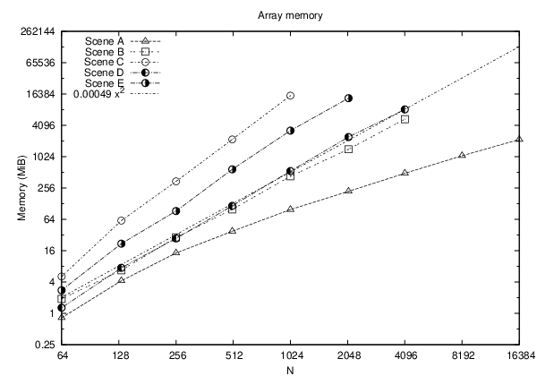
On the other hand, the saved memory is paid for by an increase in query time; cf. Figure 11b). Indeed at scenes of size $n\approx 20,000$ each query is estimated to take about $50\text{ms}$, that is as long as one frame may last at an interactive rate of $20\text{fps}$. Whereas scene E), that is scene C) with $\ell=n^{1/4}$ instead of $\ell=n^{1/2}$, is estimated to still remain far below this limit for much, much larger scenes $n$; not to mention scenes A) to C), i.e. with $\ell=1$.

Our benchmarks range up to $n\approx 8,000$ when the data structure hit an overall memory limit of 16GB. This may first seem to fall far short of the original sizes aimed at in Section 1.1. On the other hand,

• •

  the measurements obtained turn out to depend smoothly on $n$ and thus give a sufficient indication of, and permit to extrapolate with convincing significance, the behavior on larger scenes.

• •

  By proceeding from single geometric simplicies to entire ‘virtual objects’ (like e.g. a house or a car) as rendering primitives, one can in practice easily save a factor of 100 or 1000.

• •

  Temporal and spacial coherence of an observer moving within a virtual scene suggests that visibility counting queries need not be performed in each frame separately. Moreover our CPU-based algorithm can be run concurrently to the graphics processing unit (GPU). These two improvements in running time can then be traded for an additional saving in memory.

• •

  In order to attain and access the 16GB mentioned above, we employed secondary storage (a harddisk): with an unfavorable increase in preprocessing time but suprisingly little effects on the query time.

These observations suggest that our algorithm’s practicality can be extended to $n$ much larger than the above $8,000$; yet doing so is beyond the purpose of the present work.

It is thus fair to claim as main benefit of our contribution in Corollary 2 an (as opposed to Corollary 1) practically relevant approach to approximate visibility counting based on the ability to trade (otherwise prohibitive quartic) preprocessing space for (otherwise almost neglectible logarithmic) query time.

We have presented various data structures and algorithms for visibility counting, trading preprocessing space for query time. It would be most interesting to complement these results by corresponding lower bounds of the form: preprocessing space $s$ requires, in some appropriate model of computation, query time at least $\Omega\big(f(s)\big)$. Unfortunately techniques for Friedman’s Arithmetic Model, which have proven so very successful for range query problems [Chaz90], do not apply to the non-faithful semigroup weights of geometric counting problems, not to mention decision Problem 1; and approximate, rather than exact, counting makes proofs even more complicated.

On the other hand, we do have some lower bounds: namely on the sizes of VSPs and relaxed VSPs in Lemma 4a) and Proposition 1a+b). These immediately translate to lower bounds on the sizes of Linear Branching Programs, based on the observation that any such program needs a different leaf for each different convex cell of inputs leading to the same output value, compare [DFZ02].

But then again this seemingly natural model of computation is put into question when considering the algorithms from Sections 2.1 and 2.2: Both have, in spite of Lemma 4a), merely (weakly) linear size. Superficially, Lemma 2 seems to employ transcendental functions for angle calculations; but these can be avoided by comparing slopes instead of angles—however employing divisions. These, again, can be replaced: yet multiplications do remain and make the algorithm inherently nonlinear a branching program.

We had deliberately restricted to the planar case of line segments. Many virtual scenes in interactive walkthrough applications can be described as $2\tfrac{1}{2}$-dimensional: buildings of various heights yet rooted on a common plane.

But how about the full 3D case? Here we observe a quadratic ‘almost’ lower bound on the joint running time of preprocessing and querying for the 3D counterpart to Problem 1. To this end recall the following famous

It admits an easy algebraic $\mathcal{O}(n^{2})$-time algorithm but is not known solvable in subquadratic time. Similar to Boolean Satisfiability (SAT) and the theory of $\mathcal{NP}$-completeness, 3SUM has led to a rich family of problems mutually reducible one to another in softly linear time $\mathcal{O}(n\cdot\operatorname{polylog}n)$ and hence called 3SUM-complete; for example it holds [GaOv95, Section 6.1]:

In particular there is no 3D counterpart to the Interval Tree solving the corresponding 2D problem in time $\mathcal{O}(n\cdot\log n)$, recall Section 2.1.

References

- [Agar90] P. Agarwal: “Partitioning Arrangements of Lines I: An Efficient Deterministic Algorithm”, pp.449–483 in Discrete Comput. Geom. vol.5 (1990).
- [AlSp00] N. Alon, J.H. Spencer: “The Probabilistic Method”, 2nd Edition, Wiley (2000).
- [BKOS97] M. de Berg, M. van Kreveld, M. Overmars, O. Schwarzkopf: “Computational Geometry, Algorithms and Applications”, Springer (1997).
- [CAF07] S. Charneau, L. Aveneau, L. Fuchs: “Exact, Robust and Efficient Full Visibility Computation in Plücker Space”, pp.773–782 in Visual Comput. vol.23 (2007).
- [CCSD03] D. Cohen-Or, Y.L. Chrysanthou, C.T. Silva, F. Durand: “A Survey of Visibility for Walkthrough Applications”, pp.412–431 in IEEE Transactions on Visualization and Computer Graphics vol.9:3 (2003).
- [Chaz86] B. Chazelle: “Filtering Search: A New Approach to Query-Answering”, pp.703–724 in SIAM J. Comput. vol.15:3 (1986).
- [Chaz90] B. Chazelle: “Lower Bounds for Orthogonal Range Searching: II. The Arithmetic Model”, pp.439–463 in J. ACM vol.37:3 (1990).
- [DFZ02] V. Damerow, L. Finschi, M. Ziegler: “Point Location Algorithms of Minimum Size”, pp.5–9 in Proc. 14th Canadian Conf. on Computational Geometry (CCCG 2002).
- [Edel87] H. Edelsbrunner: “Algorithms in Combinatorial Geometry”, Springer (1987).
- [ELPZ07] H. Everett, S. Lazard, S. Petitjean, L. Zhang: “On the Expected Size of the 2D Visibility Complex”, pp.361–381 in Int. J. Comput. Geom. vol.17:4 (2007).
- [FJZ09] M. Fischer, C. Jähn, M. Ziegler: “Adaptive Mesh Approach for Predicting Algorithm Behavior with Application to Visibility Culling in Computer Graphics”, submitted.
- [FuSe93] T.A. Funkhouser, C.H. Séquin: “Adaptive display algorithm for interactive frame rates during visualization of complex virtual environments”, pp.247–254 in Proc. 20th Annual Conference on Computer Graphics and Interactive Techniques (SIGGRAPH’93).
- [GaOv95] A. Gajentaan, M. Overmars: “On a Class of Problems in Computational Geometry”, pp.165–185 in Computational Geometry: Theory and Applications vol.5:3 (1995).
- [GhMo91] S.K. Ghosh, D. Mount: “An Output Sensitive Algorithm for Computing Visibility Graphs”, pp.888–910 in SIAM J. Comput. vol.20 (1991).
- [Ghos07] S.K. Ghosh: “Visibility Algorithms in the Plane”, Cambridge University Press (2007).
- [HPV77] J.E. Hopcroft, W.J. Paul, L.G. Valiant: “On Time Versus Space”, pp.332–337 in Journal of the ACM vol.24:2 (1977).
- [KKF*04] J. Klein, J. Krokowski, M. Fischer, M. Wand, R. Wanka, F. Meyer auf der Heide: “The Randomized Sample Tree: A Data Structure for Externally Stored Virtual Environments”, pp.617–637 in Presence vol.13:6, MIT Press (2004).
- [Mato02] J. Matoušek: “Lectures on Discrete Geometry”, Springer Graduate Texts in Mathematics vol.212 (2002).
- [McKe87] M. McKenna: “Worst-Case Optimal Hidden Surface Removal”, pp.19–28 in ACM Transaction on Graphics vol.6 (1987).
- [MoRa95] R. Motwani, P. Raghavan: “Randomized Algorithms”, Cambridge University Press (1995).
- [ORou87] J. O’Rourke: “Art Gallery Theorems and Algorithms”, Oxford University Press (1987).
- [OvWe88] M. Overmars, E. Welzl: “New Methods for Constructing Visibility Graphs”, pp.164–171 in Proc. 4th ACM Symposium on Computational Geometry (1988).
- [PlDy90] H. Plantinga, Ch.R. Dyer: “Visibility, Occlusion, and the Aspect Graph”, pp.137–160 in Int. Journal Computer Vision vol.5:2 (1990).
- [Pocc90] M. Pocchiola: “Graphics in Flatland Revisited”, pp.85–96 in Proc. 2nd Scandinavian Workshop on Algorithms Theory, Springer LNCS vol.447 (1990).
- [PoVe96] M. Pocchiola, G. Vegter: “The Visibility Complex”, pp.279–308 in International Journal of Computational Geometry & Applications vol.6:3 (1996).
- [Schi01] R.D. Schiffenbauer: “A Survey of Aspect Graphs”, TR-CIS-2001-01 Brooklyn University (2001).
- [Tell92] S.J. Teller: “Visibility Computations in Densely Occluded Polyhedral Environments”, Dissertation University of California Berkeley (1992).
- [TeSe91] S.J. Teller, C.H. Séquin: “Visibility Preprocessing For Interactive Walkthroughs”, pp.61–69 in Computer Graphics vol.25:4 (1991).
- [WFP*01] M. Wand, M. Fischer, I. Peter, F. Meyer auf der Heide, W. Straßer: “The Randomized -Buffer Algorithm: Interactive Rendering of Highly Complex Scenes”, in Proc. 28th Annual Conference on Computer Graphics and Interactive Techniques (SIGGRAPH 2001).
- [WW*06] Peter Wonka, Michael Wimmer, Kaichi Zhou, Stefan Maierhofer, Gerd Hesina, Alexander Reshetov: “Guided visibility sampling”, in Proc. of SIGGRAPH 2006, pp. 494–502, (2006).