A string-like configuration with string tension $\varepsilon_{1}$ can be metastable with respect to either a complete breaking[1, 2] or a transition to a string of a lower tension $\varepsilon_{2}$, with $\varepsilon_{2}<\varepsilon_{1}$ [3]. The metastability arises through existence of an energy barrier due to the emergence in the process of two interfaces (the ends of the original string) each having mass $\mu$. At zero temperature the breaking of the string proceeds due to quantum tunneling and nucleation of a critical gap in the original string with the length $\ell_{c}=2\mu/(\varepsilon_{1}-\varepsilon_{2})$, at which length the energy gain due to the lower tension in the gap compensates for the energy $2\mu$ required for the formation of the interfaces. Once nucleated, the critical gap expands and converts the whole length of the original string into either a string with the lower tension, or into ‘nothing’, which formally corresponds to the limit $\varepsilon_{2}\to 0$. This mechanism of the string transition bears strong similarity[1, 2, 3] to the decay of false vacuum[4, 5] and to the Schwinger process[6] of creation of pairs of charged particles by electric field. However there is an important difference between the string transition and the latter processes. Namely, the transverse waves on the string correspond to a presence of massless degrees of freedom, which substantially affect the probability of nucleation of the critical gap. The effect of the transverse degrees of freedom has recently been calculated[10] in terms of the preexponential factor in the rate of the nucleation at zero temperature of critical gaps per length of the original string in a $d$-dimensional theory:

$${d\Gamma\over d\ell}={\varepsilon_{1}-\varepsilon_{2}\over 2\pi}\,\left[F\left({\varepsilon_{2}\over\varepsilon_{1}}\right)\right]^{d-2}\,\exp\left(-\,{\pi\,\mu_{R}^{2}\over\varepsilon_{1}-\varepsilon_{2}}\right)~,$$

(1)

with $\mu_{R}$ being the renormalized value of the mass of the interface that includes the effects of the transverse motion of the adjacent part of the string, and $F$ is the factor contributed in the rate by each of the $(d-2)$ transverse dimensions and given by

$$F(\rho)=\sqrt{{1+\rho\over 2}}\,\Gamma\left({2\over 1-\rho}\right)\,\left({1+\rho\over 1-\rho}\right)^{1+\rho\over 1-\rho}\,\exp\left({1+\rho\over 1-\rho}\right)\ \left(2\pi\,{1+\rho\over 1-\rho}\right)^{-1/2}~.$$

(2)

In this paper we consider the thermal effect in the rate of the string transition at low temperatures. This effect further exposes the difference between the breaking of a string on one side and the false vacuum decay and the Schwinger process on the other. Namely, as long as the temperature $T$ is lower than the inverse of the critical length, $T<1/\ell_{c}$ the thermal effects in the latter processes is exponentially suppressed as $\exp(-m/T)$ with $m$ being the lowest scale for particle masses in the theory, and these effects are essentially due to the (exponentially small) presence of massive particles in the thermal equilibrium[11]. In the case of a string, however, the transverse waves on the string are massless so that their excitation has no suppression by the mass at arbitrarily low temperature. The thermal excitations of these waves create fluctuations in the distribution of energy in the string which catalyze the nucleation of the critical gap. Clearly, at $T\ll 1/\ell_{c}$ the typical wavelength of the thermal waves $\lambda\sim 1/T$ is large in comparison with the critical length $\ell_{c}$, and the thermal effect in the rate is quite small, although not exponentially small. We find, as a result of the calculation to be presented in this paper, that the leading low temperature correction in the nucleation rate is given by the thermal catalysis factor

$$K=\left\{1+{\pi^{8}\over 450}\,\left({\varepsilon_{1}-\varepsilon_{2}\over 3\varepsilon_{1}-\varepsilon_{2}}\right)^{2}\,\left(\frac{\ell_{c}T}{2}\right)^{8}+O\left[(\ell_{c}T)^{12}\right]\right\}^{d-2}~.$$

(3)

We also find that as $T$ approaches $1/\ell_{c}$ the catalysis factor develops a singularity at $\ell_{c}T=1$. At still higher temperatures the considered here string transition behaves, in a sense, similarly to the false vacuum decay[11], namely the regime of the transition changes to a different tunneling trajectory, so that the temperature dependence appears in the semiclassical exponential factor in Eq.(1), rather than in the preexponential term.

The material in this paper is organized as follows. In the next Section we formulate the problem in terms of periodic configurations in Euclidean space-time, and in Sect. 3 we calculate the relevant path integrals and find the general formula for the catalysis factor in terms of expansion in powers of $\ell_{c}T$. In Sect. 4 we further analyze the general formula and find the first terms in the low temperature expansion of the catalysis factor, and also calculate this factor numerically for the temperatures approaching the critical point at $\ell_{c}T=1$. Finally, Sect. 5 contains a summary of our results.

The tunneling trajectory describing the decay of a metastable state can be found as a classical configuration, called “the bounce”, in the Euclidean space-time[5], and the exponential factor for the decay rate is given by the classical action on the bounce. The fields in the bounce configuration approach their values in the metastable state at the boundaries of the space-time and they approach the final state values inside the bounce.

In the discussed here problem of the string transition the bounce is found in terms of the effective low-energy Nambu-Goto action for the states of the string. For two strings with tensions $\varepsilon_{1}$ and $\varepsilon_{2}$ and a particle with mass $\mu$ propagating along the interface of the strings one can write the action in the form

$$S=\mu\,P+\varepsilon_{1}\,A_{1}+\varepsilon_{2}\,A_{2}~,$$

(4)

with $P$ being the perimeter of the interface and $A_{i}$ being the corresponding string’s world surface area. The approximation of the action of the system with the effective low-energy one is applicable as long as massive internal degrees of freedom of the strings are not excited. This implies in particular that the approximation is applicable only as long as the thickness of the strings can be neglected comparing to other length scales in the problem, or equivalently only as long as all the momenta in the problem are small compared to the inverse thickness of the string. If the thickness of the string is $r_{0}$ and the mass scale associated with it is $M_{0}=1/r_{0}$ then we can write the condition of applicability of the approach presented in the form

$$l\gg r_{0},\,~~~~~k\ll M_{0}$$

(5)

We consider initially a string with tension $\varepsilon_{1}$ with very large length $X$ stretched along the $x$ direction. At zero temperature the stationary configurations for the action (4) are the trivial one, which is a flat world surface of the string lying in $(t,x)$ plane, and the bounce configuration, which has a disk filled with the lower phase of the string with the radius

$$R=\frac{\mu}{\varepsilon_{1}-\varepsilon_{2}}~,$$

(6)

as shown in Fig. 1. One can readily notice that the length of the critical gap is the diameter of the disk, $\ell_{c}=2\,R$.

The condition (5) for applicability of the effective action (4) requires that

$$\frac{R}{r_{0}}\equiv M_{0}\,R={M_{0}\,\mu\over\varepsilon_{1}-\varepsilon_{2}}\gg 1~.$$

(7)

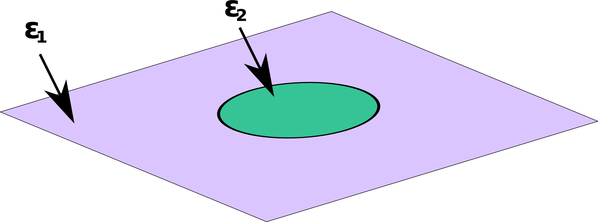
The rate of the critical gap nucleation is then found[7, 5, 8] by calculating the path integral ${\cal Z}_{12}$ around the bounce and comparing it with the path integral ${\cal Z}_{1}$ around the trivial configuration:

$${d\Gamma\over d\ell}={1\over{\cal A}}\,\mathrm{Im}\frac{{\cal Z}_{12}}{{\cal Z}_{1}}~,$$

(8)

where ${\cal A}$ is the total area of the world surface for the string. It can also be reminded that, as explained in great detail in Ref.[8], the imaginary part of ${\cal Z}_{12}$ arises from one negative mode at the bounce configuration, and that due to two translational zero modes the numerator in Eq.(8) is proportional to the total space time area ${\cal A}$ in the $(t,x)$ plane occupied by the string, so that the finite quantity is the transition probability per unit time (the rate) and per unit length of the string.

The formula in Eq.(8) corresponds to a calculation of the decay rate as the imaginary part of the energy of the initial string. At a finite temperature $T$ the corresponding relevant quantity is the imaginary part of the free energy[9], which one can calculate in the Euclidean space by considering periodic in time configurations with the period $\beta=T^{-1}$. In other words the thermal calculation corresponds to the path integration in the Euclidean space-time having the topology of a cylinder. The nucleation rate is then described by the same formula (8) with the action and the area being calculated over one period, ${\cal A}=X\,\beta$.

In the present paper we consider only sufficiently small temperatures $\beta>\ell_{c}=2\,R$, at which temperatures we find the thermal effects behaving as powers of $T$, which distinguish the string process from the decay of metastable vacuum[11]. We also treat the length $X$ of the metastable string as the largest length parameter in the problem, so that $\beta\ll X$. Under these conditions the bounce corresponding to the action (4) is the same as at zero temperature, except that it is placed on a cylinder rather than on a large flat plane (Fig. 2).

We aim at calculating the path integral over the variations of the string around the bounce configuration, which involves in particular the integration over the shifts of the string in transverse directions, i.e. those perpendicular to $x$. The contribution from each of the $d-2$ transverse dimensions factorizes, so that it is sufficient to consider only one transverse dimension with further straightforward generalization to an arbitrary dimension. The coordinates on the cylinder (or on the plane where all the points separated by $n\beta$ along Euclidean time are identified) are $t$, $x$, with $t$ being the periodic time coordinate, and the coordinate orthogonal to the surface of the cylinder is $z$. The boundary conditions for the configurations over which we integrate are

$$z\left(t,x=\pm{X\over 2}\right)=0,\,~~~~~z(t+\beta,x)=z(t,x)~.$$

(9)

Introducing the polar coordinates $(r,\theta)$ in the $(t,x)$-plane one can consider small variations of the classical configuration (Figs. 2, 3) in the following form. Variations of the interface are given by

$$r(\theta)=R+f(\theta)\,~~~~z(R,\theta)=\xi(\theta)~,$$

(10)

while the variations of the surfaces of the string in the bulk are $z_{1}(r,\theta)$ and $z_{2}(r,\theta)$ with the boundary conditions on the interface

$$z_{1}(R,\theta)=z_{2}(R,\theta)=\xi(\theta).$$

(11)

One can certainly notice that the symmetry of the polar coordinates is that of the disk describing the bounce, but it is not the symmetry of the periodicity condition in $t$. It will be clear from the subsequent calculation, that in fact all the discussed thermal effect can be viewed as originating from this mismatch, once it is properly accounted for.

In terms of the introduced variables the action (4) can be written in the quadratic approximation in the deviations from the bounce as

	$\displaystyle S_{12}=\varepsilon_{1}\,X\,\beta+{\pi\,\mu^{2}\over\varepsilon_{1}-\varepsilon_{2}}+{\varepsilon_{1}-\varepsilon_{2}\over 2}\,\int d\theta\,\left(\dot{\xi}^{2}+\dot{f}^{2}-f^{2}\right)+$
	$\displaystyle{\varepsilon_{1}\over 2}\,\int_{\rm out}rdrd\theta\,\left(z_{1}^{\prime}\,{}^{2}+{\dot{z_{1}}^{2}\over r^{2}}\right)+{\varepsilon_{2}\over 2}\,\int_{\rm in}rdrd\theta\,\left(z_{2}^{\prime}\,{}^{2}+{\dot{z_{2}}^{2}\over r^{2}}\right)~,$		(12)

where the primed and dotted symbols stand for the derivatives with respect to $r$ and $\theta$ correspondingly, and the “out” and “in” integrals are taken over the surface respectively outside and inside the disk $r<R$.

Similarly, the action around a flat initial string configuration in the quadratic approximation takes the form

$$S_{1}=\varepsilon_{1}\,X\,\beta+{\varepsilon_{1}\over 2}\,\int rdrd\theta\,\left(z^{\prime}\,{}^{2}+{\dot{z}^{2}\over r^{2}}\right)~,$$

(13)

with the integral running over the whole space-time cylinder and $z(r,\theta)$ parametrizing small deviations of the string in the transverse direction.

The path integral ${\cal Z}_{1}$ runs all transverse fluctuations $z(r,\theta)$ with the action given by Eq.(13). This integral contains no interface at $r=R$. However, as explained in Ref. [10], for the purpose of calculation of the ratio of the partition functions in Eq.(8) it is helpful to organize the integration for ${\cal Z}_{1}$ in the following way. First one fixes the values of $z$ on the circle of radius $R$: $z(R,\theta)=\xi(\theta)$, and integrates over the remaining bulk variables with fixed $\xi(\theta)$. The full partition function ${\cal Z}_{1}$ is then found after path integration over the boundary variations $\xi(\theta)$. As demonstrated in Ref. [10] this procedure in fact factorizes the full path integral into a product of “bulk” and “boundary” factors with the bulk factors being the same in ${\cal Z}_{12}$ and ${\cal Z}_{1}$. As a result the ratio of the full path integrals in Eq.(8) is determined only by the boundary terms:

$${d\Gamma\over d\ell}={\varepsilon_{1}-\varepsilon_{2}\over 2\pi}\,\exp\left(-{\pi\,\mu^{2}\over\varepsilon_{1}-\varepsilon_{2}}\right)\,\,{{\cal Z}_{12{\rm(boundary)}}\over{\cal Z}_{1{\rm(boundary)}}}~$$

(14)

with the boundary partition functions ${\cal Z}_{12(\rm boundary)}$ and ${\cal Z}_{1(\rm boundary)}$ being given by

	$\displaystyle{\cal Z}_{12(\rm boundary)}=\int{\cal D}\xi\,\exp\left[-{\varepsilon_{1}-\varepsilon_{2}\over 2}\,\int d\theta\,\dot{\xi}^{2}-R\,\int d\theta\,\left({\varepsilon_{2}\over 2}{\partial_{r}}z_{2c}\left.\right|_{r=R}-{\varepsilon_{1}\over 2}{\partial_{r}}z_{1c}\left.\right|_{r=R}\right)\,\xi\right]$
	$\displaystyle{\cal Z}_{1(\rm boundary)}=\int{\cal D}\xi\,\exp\left[-R\,{\varepsilon_{1}\over 2}\,\int d\theta\,\left({\partial_{r}}z_{2c}\left.\right|_{r=R}-{\partial_{r}}z_{1c}\left.\right|_{r=R}\right)\,\xi\right]~,$		(15)

where the functions $z_{1c}$ and $z_{2c}$ satisfy the Laplace equation $\Delta z_{ic}=0$ with the boundary conditions

$$z_{1c}(R,\theta)=z_{2c}(R,\theta)=\xi(\theta)~.$$

(16)

The outer solution $z_{1c}$ is also periodic in time $z_{1c}(t+\beta,x)=z_{1c}(t,x)$ and satisfies the zero boundary condition at the spatial infinity

$$z_{1c}\left(t,x=\pm{X\over 2}\right)=0$$

(17)

while the inner solution $z_{2c}$ is required to be regular inside the disk.

In order to do the path integrals one can expand the boundary function $\xi(\theta)$ in angular harmonics:

$$\xi(\theta)={a_{0}\over\sqrt{2\pi}}+{1\over\sqrt{\pi}}\sum_{n=1}^{\infty}\left[a_{n}\,\cos(n\theta)+b_{n}\,\sin(n\theta)\right].$$

(18)

For the inner solution $z_{2c}$ to the Laplace equation, i.e. at $r\leq R$ one finds no difficulty in finding the harmonics matching the boundary function at the interface[10]:

$$z_{2c}^{(0)}={a_{0}\over\sqrt{2\pi}}\,,~~~~z_{2c}^{(n)}(r,\theta)={1\over\sqrt{\pi}}\,\left[a_{n}\,\cos(n\theta)+b_{n}\,\sin(n\theta)\right]\,{r^{n}\over R^{n}}~.$$

(19)

For the outer solution $z_{1c}$ however there is a difficulty due to the previously mentioned mismatch between the symmetry of the boundary and of the periodicity conditions. It is impossible to choose the solution to the Laplace equation for outer string bulk variable to be $z_{1c}^{(n)}(r,\theta)\sim r^{-n}$, since it is not periodic in time. In this situation in order to have a periodic solution one can perform a periodic mapping of the cylinder on the plane and consider the outer solution of the Laplace equation as the sum of the solutions produced by a “source” at each period as illustrated in Fig. 4. Introducing the complex variable $w=t+i\,x$, we construct the solutions for the functions $z_{1c}(r,\theta)$ using the harmonic real and imaginary parts of the following basis set of periodic functions, satisfying the boundary condition (17) at large $|x|$,

	$\displaystyle g_{0}(w)$	$\displaystyle=$	$\displaystyle\ln\left[\sin\left(\frac{\pi\,w}{\beta}\right)\right]-{\pi\,X\over 2\beta}-i\,{\pi x\over X}+\ln 2~,$
	$\displaystyle g_{1}(w)$	$\displaystyle=$	$\displaystyle\frac{\pi\,R}{\beta}\,\cot\left(\frac{\pi\,w}{\beta}\right)+i\,{2\,\pi\,R\,x\over\beta\,X}~,$
	$\displaystyle{g}_{k}(w)$	$\displaystyle=$	$\displaystyle\frac{R^{k}}{w^{k}}+\sum_{n=1}^{\infty}\left[\frac{R^{k}}{(w-n\beta)^{k}}+\frac{R^{k}}{(w+n\beta)^{k}}\right],~~~\textrm{for $k>1$}~.$		(20)

Clearly these functions are periodic in the Euclidean time by construction, with the period $\beta$. Also the functions $g_{k}(w)$ with $k>1$ are analytic complex functions, so that their real and imaginary parts are harmonic. In the functions $g_{0}(w)$ and $g_{1}(w)$ the explicit dependence on $x$, introducing non-analyticity, is linear and is thus also harmonic, so that their real and imaginary parts do satisfy the Laplace equation.

An arbitrary periodic outer solution to the Laplace equation, satisfying the boundary condition (17) at large $|x|$ can be expanded in the series

$$z_{1c}(r,\theta)=A_{0}\mathrm{Re}\,g_{0}(w)+\sum_{k=1}^{\infty}A_{k}\mathrm{Re}\,g_{k}(w)+B_{k}\mathrm{Im}\,g_{k}(w),$$

(21)

The disadvantage of this set of solutions (hence of such an expansion) is that it is not orthogonal, so that the expression for the action up to quadratic terms is not diagonal in this basis. Therefore, the calculation of the integral is not just a calculation of the product of eigenvalues. To find the integral over the amplitudes of the Fourier harmonics one has to express the amplitudes of the solutions chosen $A_{k}$,$B_{k}$ in terms of the amplitudes $a_{k}$, $b_{k}$. The relation between the coefficients $A_{k}$,$B_{k}$ and $a_{k}$, $b_{k}$ can be found from the matching condition (16) on the interface

$${a_{0}\over\sqrt{2\pi}}+{1\over\sqrt{\pi}}\sum_{n=1}^{\infty}\left[a_{n}\,\cos(n\theta)+b_{n}\,\sin(n\theta)\right]=A_{0}\,g_{0}(w)\Big|_{r=R}+\sum_{k=1}^{\infty}\left[A_{k}\mathrm{Re}g_{k}(w)+B_{k}\mathrm{Im}g_{k}(w)\right]\Big|_{r=R}.$$

(22)

One can readily notice that the function $g_{0}$ contains a large constant term, proportional to $X$, which totally dominates the matching condition for the $a_{0}$ mode at $r=R$, so that

$${a_{0}\over\sqrt{2\pi}}=-A_{0}\,\frac{\pi\,X}{2\beta}\,\left[1+O(R/X)\right].$$

(23)

For this reason the effect of the mixing between $a_{0}$ and higher modes is suppressed by inverse powers of $X$ and can be ignored in the limit of a long string. For this reason in considering the mixing of the modes in the following calculation we keep only $k\neq 0$. Furthermore the linear in $x$ terms in the functions $g_{0}$ and $g_{1}$ are suppressed at $r=R$ by the factor $R/X$ and we also neglect them.

In what follows we consider the expansion of the functions $g_{k}$ at $r=R$ in powers of $R/\beta$, which expansion, as will be seen later, converges at $R<\beta/2$. Using

$$(1+x)^{-k}=1+\sum_{p=1}^{\infty}(-1)^{p}x^{p}C_{p+k-1}^{p},$$

(24)

where $C_{p+k-1}^{p}$ are binomial coefficients,

$$C_{p+k-1}^{p}=\frac{(p+k-1)!}{p!(k-1)!}$$

(25)

and also a definition of the Riemann $\zeta$-function

$$\zeta(k)=\sum_{n=1}^{\infty}n^{-k}~,$$

(26)

we find for $k\neq 0$

$$g_{k}(w)=\frac{R^{k}}{w^{k}}+\sum_{p=1}^{\infty}d_{pk}\left(\frac{w}{R}\right)^{p},$$

(27)

with

$$d_{pk}=\left[(-1)^{k}+(-1)^{p}\right]\left(\frac{R}{\beta}\right)^{k+p}\,\zeta(p+k)\,C_{p+k-1}^{p}.$$

(28)

We have omitted in the expression (27) a constant term, which describes the mixing with the $a_{0}$ mode as well as a term explicitly proportional to $R/X$. Using the expansion (27) for $g_{k}(w)$ and considering the real part of the functions $g_{k}(w)$, one can find the coefficients $a_{l}$ in terms of $A_{k}$

$$a_{l}=\frac{1}{\pi}\sum_{k}A_{k}\int_{0}^{2\pi}\mathrm{Re}g_{k}\cos(l\theta)d\theta=A_{l}+\sum_{k=1}^{\infty}A_{k}\,d_{lk}~,$$

(29)

or in the matrix form

$$A=(1+D)^{-1}\,a~,$$

(30)

where matrix $D$ has elements $d_{lk}$. Similarly for the imaginary part one gets

$$b_{l}=\frac{1}{\pi}\sum_{k}B_{k}\int_{0}^{2\pi}\mathrm{Im}g_{k}\cos(l\theta)d\theta=B_{l}-\sum_{k}B_{k}d_{lk}$$

(31)

and

$$B=(1-D)^{-1}\,b~.$$

(32)

As usual, the contributions from $\cos$ and $\sin$ modes are independent, and we consider the contribution to the boundary term in (15) from the even ($\cos$) harmonics first

	$\displaystyle-\int_{0}^{2\pi}\left.\left(Rg^{(R)}\partial_{r}g^{(R)}\right)\right|_{R}d\theta=\int_{0}^{2\pi}d\theta\left[\sum_{l}a_{l}\ cos(l\theta)\right]\sum_{k}\left[k\left(\frac{R}{r}\right)^{k}\cos(k\theta)-\sum_{p=1}^{\infty}pd_{pk}\right]=$
	$\displaystyle\sum_{k}A_{k}\left[ka_{k}-\sum_{p}pa_{p}d_{pk}\right]=\sum_{k,p}a_{p}\left[k\delta_{pk}-pd_{pk}\right]A_{k}~.$		(33)

Introducing the matrix

$$\hat{N}=\mathrm{diag}(1,2,\dots,n,\dots)~,$$

(34)

one can rewrite the expression (33) in the matrix form

$$-\int_{0}^{2\pi}\left.\left(Rg^{(R)}\partial_{r}g^{(R)}\right)\right|_{R}d\theta=a\hat{N}(1-D)A~.$$

(35)

A substitution in this expression of the solution for $A$ in terms of $a$ (30) leads to

$$-\int_{0}^{2\pi}\left.\left(Rg^{(R)}\partial_{r}g^{(R)}\right)\right|_{R}d\theta=a\hat{N}(1-D)(1+D)^{-1}a~.$$

(36)

Clearly, for the odd ($\sin$) modes one gets the same expression with the replacement $D\to-D$. Collecting all the terms together one can write the result for the boundary partition functions (15) as

	$\displaystyle{\cal Z}_{12(\rm boundary)}$	$\displaystyle=$	$\displaystyle\mathrm{Det}\left[(\varepsilon_{1}-\varepsilon_{2})\hat{N}^{2}+\varepsilon_{2}\hat{N}+\varepsilon_{1}\hat{N}(1-D)\frac{1}{1+D}\right]^{-1/2}\cdot\{D\to-D\}$
	$\displaystyle{\cal Z}_{1(\rm boundary)}$	$\displaystyle=$	$\displaystyle\mathrm{Det}\left[\varepsilon_{1}\hat{N}+\varepsilon_{1}\hat{N}(1-D)\frac{1}{1+D}\right]^{-1/2}\cdot\{D\to-D\},$		(37)

where $\{D\to-D\}$ means that one should take the expression and make the replacement $D\to-D$.

The zero temperature limit for the probability rate $d\Gamma_{0}/d\ell$ formally corresponds to setting $D\to 0$. Thus one can use the known result for the zero temperature decay rate [10], and concentrate on a calculation of the thermal catalysis factor $K$ defined as

$$\frac{d\Gamma}{d\ell}=K\,\frac{d\Gamma_{0}}{d\ell}\,.$$

(38)

In a $d$-dimensional theory, i.e. with $d-2$ transverse dimensions, the catalysis factor can be written as $K=G^{d-2}$, where $G$ is the factor per each transverse direction given by

$$G=\frac{{\cal Z}_{12(\rm boundary)}}{{\cal Z}_{12(\rm boundary)}^{D=0}}\,\frac{{\cal Z}_{1(\rm boundary)}^{D=0}}{{\cal Z}_{1(\rm boundary)}}\,.$$

(39)

According to Eq.(37) it is a matter of simple algebra to express the factor $G$ in terms of the matrix $D$:

$$G=\mathrm{Det}\left[1-\left(\frac{\hat{N}-1}{\hat{N}+b}\,D\right)^{2}\right]^{-1/2}$$

(40)

where we have introduced the parameter $b=\displaystyle\frac{\varepsilon_{1}+\varepsilon_{2}}{\varepsilon_{1}-\varepsilon_{2}}$.

In this section we consider in some detail the temperature effect in the string transition rate described by our general formula (40) in the situation where the inverse temperature is larger then the diameter of the classical configuration (bounce) $\beta>2R$. We first notice that due to the presence of the factor $(\hat{N}-1)$ the first elements from the first row and the first column of the matrix $D$, $d_{1k}$ and $d_{p1}$, enter the expression $[(\hat{N}-1)\,D]^{2}$ with zero coefficients, so that the final result (40) does not depend on them. Furthermore, one can see from Eq.(28) that the matrix element $d_{pk}$ is not equal to zero only if the indices $p$ and $k$ have the same parity. Hence, there is no mixing between the amplitudes with even ($a_{2l}$, $b_{2l}$) and odd ($a_{2l+1}$, $b_{2l+1}$) indices. Therefore the determinant in the (40) can be written as a product of determinants corresponding to even and odd amplitudes

$$\mathrm{Det}\left[1-\left(\frac{\hat{N}-1}{\hat{N}+b}\,D\right)^{2}\right]=\mathrm{Det}\left[1-\left(\frac{2\,\hat{N}-1}{\hat{2\,N}+b}\,U\right)^{2}\right]\,\mathrm{Det}\left[1-\left(\frac{2\,\hat{N}}{2\,\hat{N}+1+b}\,V\right)^{2}\right],$$

(41)

where the matrix elements of the matrices $U$ and $V$ are

$$U_{pk}=d_{2p\,2k}\,,~~~~~V_{pk}=d_{2p+1,\,2k+1}~,$$

(42)

and the indices $p$ and $k$ take values $1,2,\ldots$ .

For practical calculations it is also convenient to write the expressions for the elements of the matrices entering in Eq.(41) in terms of their indices:

	$\displaystyle\left(\frac{2\,\hat{N}-1}{\hat{2\,N}+b}\,U\right)_{pk}$	$\displaystyle=$	$\displaystyle 2\,{2p-1\over 2p+b}\,{(2p+2k-1)!\over(2p)!\,(2k-1)!}\,\zeta(2p+2k)\,\left({R\over\beta}\right)^{2p+2k}~,$
	$\displaystyle-\left(\frac{2\,\hat{N}}{2\,\hat{N}+1+b}\,V\right)_{pk}$	$\displaystyle=$	$\displaystyle{4p\over 2p+1+b}\,{(2p+2k+1)!\over(2p+1)!\,(2k)!}\,\zeta(2p+2k+2)\,\left({R\over\beta}\right)^{2p+2k+2}~,$		(43)

with $p,k=1,2,\ldots$.

In order to find the first thermal correction at low temperature one can expand the matrices in power series using well known formula for the determinant

$$\mathrm{Det}(1-M)=\exp\left[\mathrm{Tr}\ln\left(1-M\right)\right]=\exp\left[-\mathrm{Tr}\sum_{l=1}^{\infty}\frac{M^{l}}{l}\right]=1-\mathrm{Tr}M+O(M^{2}).$$

(44)

In our case

$$\left(\frac{2\,\hat{N}-1}{2\,\hat{N}+b}\,U\right)^{2}=\left(\begin{array}[]{ccc}\displaystyle\frac{36\,\zeta^{2}(4)}{(2+b)^{2}}\left(\frac{R}{\beta}\right)^{8}+\frac{600\,\zeta(6)^{2}}{(2+b)\,(4+b)}\,\left(\frac{R}{\beta}\right)^{12}&\displaystyle\frac{120\,\zeta(4)\zeta(6)}{(2+b)^{2}}\,\left(\frac{R}{\beta}\right)^{10}&\cdots\\ \displaystyle\frac{180\,\zeta(4)\zeta(6)}{(2+b)\,(4+b)}\,\left(\frac{R}{\beta}\right)^{10}&\displaystyle\frac{600\,\zeta(6)^{2}}{(2+b)\,(4+b)}\,\left(\frac{R}{\beta}\right)^{12}&\cdots\\ \vdots&\vdots&\ddots\end{array}\right)~,$$

(45)

$$\left(\frac{2\,\hat{N}}{2\,\hat{N}+1+b}\,V\right)^{2}=\left(\begin{array}[]{cc}\displaystyle\displaystyle\frac{1600\,\zeta(6)^{2}}{(3+b)^{2}}\,\left(\frac{R}{\beta}\right)^{12}&\cdots\\ \vdots&\ddots\end{array}\right)~.$$

(46)

Therefore the first correction to the zero temperature value of the rate is proportional to $R^{8}/\beta^{8}$ and is given by Eq.(3).

The series for the function $G(T)$ diverges when $\beta=2\,R$. The corrections for the temperature close to $(2R)^{-1}$ can be found numerically. The proximity to this point defines the number of terms which should be taken into account in the series for $G(T)$. The plot for the function $G(T)$ vs the parameter $R/\beta=R\,T$ calculated numerically with 50 first rows and columns retained in the matrices $U$ and $V$ is shown in Fig. 5.

In the present paper we considered the transition between two states of a string at finite temperature. The result for the rate of the transition in arbitrary number of dimensions is obtained in a form of a product of the value at zero temperature and the catalysis factor (40). The numerical analysis of the expression shows (see Fig.5) that for smaller $b$ the influence of the temperature on the process becomes noticeable earlier and the catalysis factor grows more rapidly with temperature. Our result is applicable in the range of temperatures for which the associated period in Euclidean time is larger then the critical size of the classical configuration $\ell_{c}\,T>1$, so that it is still possible to inscribe the bounce in one period. We have shown that, similarly to the process of false vacuum decay at finite temperature in two dimensions [11], there is no change in the exponential behavior of the probability rate while the temperature is small enough, and that such change starts only when $\beta$ becomes smaller than the diameter of the bounce. On the other hand we have demonstrated that unlike in the case of false vacuum decay, there arise thermal corrections to the transition rate at low temperature, which corrections have power dependence on the temperature and are due to thermal waves excited on the string at arbitrarily low temperatures. In practical terms, as can be seen from Fig. 5, the value of the catalysis factor changes from $1$ for $R\,T=0$ to approximately $1.5$ for $R\,T=0.49$, i.e. quite slowly, even for $b=1$. However there is an actual singularity in this factor at $R\,T=1/2$ so that the string transition becomes significantly accelerated by thermal effects for temperatures close to $1/\ell_{c}$.

This work is supported in part by the DOE grant DE-FG02-94ER40823.

References

- [1] A. Vilenkin, Nucl. Phys. B 196, 240 (1982).
- [2] J. Preskill and A. Vilenkin, Phys. Rev. D 47, 2324 (1993) [arXiv:hep-ph/9209210].
- [3] M. Shifman and A. Yung, Phys. Rev. D 66, 045012 (2002) [arXiv:hep-th/0205025].
- [4] M. B. Voloshin, I. Y. Kobzarev and L. B. Okun, Sov. J. Nucl. Phys. 20, 644 (1975) [Yad. Fiz. 20, 1229 (1974)].
- [5] S. R. Coleman, Phys. Rev. D 15, 2929 (1977) [Erratum-ibid. D 16, 1248 (1977)].
- [6] J. Schwinger, Phys. Rev. 82, 664 (1951).
- [7] M. Stone, Phys. Rev. D 14, 3568 (1976).
- [8] C. G. Callan and S. R. Coleman, Phys. Rev. D 16, 1762 (1977).
- [9] J. S. Langer, Ann. Phys. (N.Y.) 41, 108 (1967).
- [10] A. Monin, M. B. Voloshin, arXiv:0808.1693
- [11] J. Garriga, Phys. Rev. D 49, 5497 (1994)