Direct Mediation, Duality and Unification
Abstract:
It is well-known that in scenarios with direct gauge mediation of supersymmetry breaking the messenger fields significantly affect the running of Standard Model couplings and introduce Landau poles which are difficult to avoid. Among other things, this appears to remove any possibility of a meaningful unification prediction and is often viewed as a strong argument against direct mediation. We propose two ways that Seiberg duality can circumvent this problem. In the first, which we call “deflected-unification”, the SUSY-breaking hidden sector is a magnetic theory which undergoes a Seiberg duality to an electric phase. Importantly, the electric version has fewer fundamental degrees of freedom coupled to the MSSM compared to the magnetic formulation. This changes the -functions of the MSSM gauge couplings so as to push their Landau poles above the unification scale. We show that this scenario is realised for recently suggested models of gauge mediation based on a metastable SCQD-type hidden sector directly coupled to MSSM. The second possibility for avoiding Landau poles, which we call “dual-unification”, begins with the observation that, if the mediating fields fall into complete multiplets, then the MSSM+messengers exhibits a fake unification at unphysical values of the gauge couplings. We show that, in known examples of electric/magnetic duals, such a fake unification in the magnetic theory reflects a real unification in the electric theory. We therefore propose that the Standard Model could itself be a magnetic dual of some unknown electric theory in which the true unification takes place. This scenario maintains the unification prediction (and unification scale) even in the presence of Landau poles in the magnetic theory below the GUT scale. We further note that this dual realization of grand unification can explain why Nature appears to unify, but the proton does not decay.
1 Introduction
One of the key questions of supersymmetric BSM particle physics is the nature of supersymmetry breaking in the hidden sector and its mediation to the visible Standard Model sector. A particularly concise and appealing proposal is the direct gauge mediation approach [1] in which the supersymmetry-breaking sector couples directly to the MSSM with no need for an additional messenger sector.
The central issue we wish to address in this paper applies particularly to models of direct gauge mediation and is this. In direct gauge mediation, supersymmetry (SUSY) is broken in a hidden sector that contains a large global flavour group which is gauged and identified with the gauge group of the Supersymmetric Standard Model (SSM) or a subgroup thereof. Supersymmetry breaking is mediated by messengers that are charged under both groups [1, 2]. Being charged under the hidden sector gauge symmetry, these direct messengers are in effect a large number of additional matter fields for the visible sector11 1 In general we will refer to the supersymmetric Standard Model including direct messengers as the SSM. We will reserve ”MSSM” to refer to the minimal model on its own (without messengers). . Consequently they give a large positive contribution to the -functions above the messenger scale, , and the visible sector gauge couplings then encounter Landau poles below at which point the perturbative description breaks down. Thus to use direct gauge mediation one has apparently to abandon perhaps the most successful prediction of the MSSM, namely gauge unification. This is often cited as evidence against it.
Here we wish to propose that theories with Landau poles can still have meaningful and predictive unification taking place ‘‘across a Seiberg duality’’ in a microscopic electric dual description.22 2 Other mechanisms of avoiding Landau poles have also been considered in the literature, including [3, 4, 5] and most recently in [6]. The Seiberg duality can be applied either to just the hidden sector or may also include the visible sector. In the former case the universal change of slopes provided by messengers in complete multiplets persists, but the slopes can change a number of times as the hidden sector goes through one or more dualities. This is a form of “deflected-unification” (to borrow a term from anomaly mediation) as shown schematically in figure 1. Similar deflection of course happens in purely perturbative theories whenever a threshold is crossed, but this always results in an increase in the effective number of flavours which only accelerates the running to Landau poles. The important feature that the Seiberg duality [7] brings is a reduction in the number of elementary direct messenger fields when one switches from the IR magnetic to the UV electric formulation of the hidden sector theory. This reduction affects the -function slopes in the SSM and moves the Landau poles to the UV or conceivably even removes them entirely. Note that the slope in the visible sector changes in this way only because the mediation is direct; from the point of view of the visible sector the electric theory simply has a different number of messenger flavours contributing in the one-loop -functions.
What solves the problem of Landau poles in this class of direct mediation scenarios is the assumption that the SUSY-breaking sector has an electric dual in the UV. Remarkably, this is precisely what happens in the Intriligator, Seiberg and Shih (ISS) model [8]. In the ISS case Seiberg duality was instrumental in achieving dynamical SUSY-breaking (DSB) in a metastable vacuum. Now, when the ISS-type model is used as the hidden sector for direct mediation of SUSY-breaking to the SSM [9, 10, 11, 12, 13], it not only provides us with a simple satisfactory description of DSB, it also resolves the Landau pole problem of direct mediation. In Section 2 we will show how this works in the context of the direct mediation models introduced in [11, 12].

The complementary possibility is that the duality takes place in the visible sector as well. One hint that unification may be preserved under such a duality has been noted by several authors in this context including most recently in ref.[13], and is the following: in a model of direct gauge mediation with messengers in complete multiplets the extra contributions to -functions are degenerate; they run to strong coupling well below , however the relative running is unchanged, so the three gauge couplings of the SSM still appear to unify at the scale , but at unphysical, negative values of . Could this fake unification be a remnant of a real unification in the electric theory?
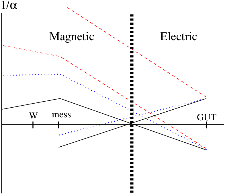
In this paper (Sections 3-4) we will see that indeed it can be: unification in the electric description leads to a “fake” unification in the magnetic one at the same energy scale but at unphysical (i.e. negative) values of . This occurs where the entire unified electric theory is dualized (i.e. if we are thinking of the SSM, then every subgroup of the SSM gets dualized). The generic picture, which we call “dual-unification”, is as sketched in figure 2. We show that a large class of known electric/magnetic duals exhibit dual-unification, and that under very general assumptions it is guaranteed by the matching relations between the electric and magnetic theories.
Finally, in Section 5 we argue that the dual-unification scenario has significant implications for the question of proton decay. While it is well-known that in the usual simple MSSM-GUT picture the lifetime of the proton turns out to be shorter than experimental bounds, we will show that in the dual-unification set-up proton decay processes can be enormously suppressed. This is due to the fact that the dangerous baryon number violating operators are induced in the electric theory where the unification takes place. At this energy scale the magnetic theory is strongly coupled and one must instead use the weakly coupled electric theory description, and then map to the low energy magnetic theory with well know baryon baryonelec identifications. This introduces many powers of making proton decay completely negligible.
2 Deflected-unification
One of the most interesting and appealing properties of supersymmetric theories is the holomorphy and nonrenormalizability of their superpotentials; from these two properties many powerful statements follow about the nonperturbative effects of strong coupling. In particular in a large number of celebrated examples beginning with SQCD models[7], one can find two (or more) dual theories that describe the same IR physics (for a review see refs.[14, 15]). For certain choices of parameters, a theory can enjoy two perturbative regimes, an asymptotically free electric one that accurately describes the UV physics and a free magnetic phase that describes the IR physics. This is the situation that will be of interest for this paper.
Let us see how such electric/magnetic duality can effect unification in simple direct mediation. We will consider a theory in which a hidden sector couples directly to the visible sector through bifundamental fields, charged under both the visible and hidden gauge groups. As described in the Introduction, if the hidden sector gauge group undergoes a duality at some energy scale, then the number of flavours seen by the visible sector also changes at that scale. If the multiplets coupling hidden to visible sector are in complete ’s as is often assumed in gauge mediation, then the nett effect will be a universal change of slope which can allow unification where in the magnetic theory it appears to be impossible.
A simple example is provided by the model of refs.[11, 12]. This is a model of direct gauge mediation with a supersymmetry breaking ISS sector [8] with , and . This sector becomes strongly coupled at a scale , and can be described by an IR free magnetic theory below that scale. The relevant quiver diagrams are shown in figure 3.

The fields and charges of the magnetic formulation are shown in Table 1,
| 1 | 2 | |||
and the superpotential is given by
| (1) |
where are flavour indices, run over the first two flavours only, and are indices (we set the Yukawa coupling to unity for simplicity). By a gauge and flavour rotation, the matrix can be brought to a diagonal form
| (2) |
We will assume that . As explained in [8], the “rank-condition” leads to metastable SUSY breaking such that . The parameters , and have an interpretation in terms of the electric theory: and come from the electric quark masses , , where is the dynamical scale of the ISS sector. The last term in (1) is the baryon deformation of the ISS model. As explained in [11, 12] it is needed to trigger spontaneous breaking of the -symmetry – by generating as well as , , – required for non-zero gaugino masses in SSM. This baryon operator can be identified with a corresponding operator in the electric theory.
In this model there is no separate mediating sector, but the flavour symmetry is explicitly broken to . The subgroup is gauged and associated with the parent of the Standard Model. The matter fields charged under this play the role of direct messengers; these are the magnetic quarks together with the meson components , and .
Now, as frequently occurs in direct mediation there is a Landau pole in the SSM as well as the ISS sector, because of the large number of additional flavours. Indeed an estimate was made in ref.[11] of where this occurs. In the magnetic theory the magnetic quarks , contribute to the -function, and the magnetic mesons contribute (the coming from the off-diagonal entries, , and the from the adjoint, ). Thus one can estimate
| (3) |
and hence
| (4) |
where is the effective messenger scale, and where here and throughout we will be using for convenience the convention that
rather than the more usual . To avoid an SSM Landau pole before unification one requires
| (5) |
or GeV, which is orders of magnitude above what one wants for normal gauge mediation. (Indeed such a high value is close to the gravity mediation scale.)
However this estimate takes no account of the change of slope in the electric ISS formulation, which is the appropriate description of the Hidden sector above the scale . Indeed the lower limit on the latter is only of order GeV [12], and above the scale the contribution to the SSM -functions comes from the “flavours” of electric quarks and antiquarks, and is just . (The mesons are composite objects in the electric dual and do not contribute to the SSM -functions as independent degrees of freedom.) Taking this change of slope into account, the gauge couplings are therefore
| (6) |
A Landau pole appears if
| (7) | |||||
Clearly minimizing ameliorates the Landau pole, so assuming that we require to avoid Landau poles or
This requirement is easily met by the phenomenological models of ref.[12].
Thus slopes can change upon Seiberg dualizing, and in particular there can be a reduction of the effective number of messengers in a model of direct gauge mediation, that delays the onset of Landau poles to beyond the GUT scale. This is a very simple example of how duality and unification can be interrelated. The main point of interest is that rather than the familiar case whereby some degrees of freedom are “integrated in” at higher energy scales, there is instead a reduction in the effective degrees of freedom.
One can generalize the discussion to arbitrary numbers of flavours and colours. The general condition for avoiding a Landau pole in this scenario is
| (8) |
where () are the -functions of the magnetic(electric) theories. For example, generalizing the model above so that the SSM is embedded in and there are flavours in the supersymmetry breaking ISS sector gives the condition
| (9) |
Note that the matching of the electric and magnetic theories in the running of the one loop gauge coupling is well understood. Indeed the electric and magnetic hidden sector gauge theories have dynamical scales related by a matching relation such as
| (10) |
where is an undetermined scale (not to be confused with in (1)) relating the composite mesons of the electric theory to the elementary meson in the magnetic theory . Since is unknown, we may choose it so that and there is a perturbative overlap of the two theories.
3 An example of visible sector dual-unification
We now turn to the complementary class of scenarios where the dynamics of the Hidden sector plays little or no role in the Landau pole problem of the Visible sector. Consider the possibility that the SSM is itself a magnetic dual theory which becomes strongly coupled and develops Landau poles above the messenger scale. As we have said, this is natural in many scenarios of gauge mediation, and if the mediating fields appear in complete multiplets the SSM unification still occurs but at unphysical values of the gauge couplings. If this is the case, is it possible that this ”fake” gauge unification is simply a manifestation of a real unification taking place in an electric dual theory? In fact there are examples in the literature of electric/magnetic dual GUT theories, which we can examine to answer this question (in the positive of course). As our prototypical example we will look at the model of Kutasov, Schwimmer and Seiberg (KSS) [16, 17] (see refs.[18, 19, 20, 21] for related work). In the following two subsections we briefly review its details, and then discuss dual-unification in subsection 3.3 and present explicit examples with magnetic in 3.4.
3.1 The electric theory
The microscopic theory is an gauge theory with flavours of quarks and anti-quarks , and an adjoint field of the , . The superpotential defining the model is
| (11) |
where are constants and is a fixed integer. The constant is the Lagrange multiplier which ensures tracelessness of . The leading term in (i.e. the term with the highest power of ) is , and the subleading terms with are often thought of as deformations. The parent global symmetry of the theory when only the leading term is present is
with the charges shown in Table 2.
| 1 | 1 | |||
| 1 | -1 | |||
| 1 | 1 | 0 |
When there are non-zero the -symmetry is completely broken. These deformations are responsible for generating the VEV for and spontaneously breaking the gauge symmetry as we shall see. KSS also use an equivalent form of this superpotential,
| (12) |
where is shifted by and the constants and are chosen in terms of and so that the coefficient of the first subleading term is zero (with ). This form is useful for ensuring that traceless adjoints in the magnetic theory are consistent with the vacuum structure.
The -term equation for non-zero ’s can easily be solved by diagonalizing the using rotations and dictates the vacuum structure; the equation for a single entry on the diagonal is
| (13) |
This is a order polynomial so there are roots; hence
| (14) |
where
| (15) |
The original microscopic gauge group is broken (Higgsed) down to
| (16) |
with the values of the roots being fixed in terms of the ’s (these are not flat directions). Around each such vacuum the adjoint field is massive and can be integrated out. The resulting theory at energy scales below (or more precisely, below the scales set by the differences ) is the product of ordinary SQCD theories times Abelian SQED-like factors (which are essentially gauged baryon numbers).
The microscopic electric will here play the role of the Grand Unified Theory; the unification above the scale(s) is by default, since we started from the single gauge group. For simplicity we will always assume that the original theory is well-defined in the UV, i.e. is asymptotically free. Its one-loop -function coefficient
| (17) |
must therefore be positive. (Here comes from the adjoint field .) The dynamical transmutation scale of this theory we will take to be .
3.2 The magnetic theory
Now let us go to the macroscopic theory, starting with the dual of the unbroken microscopic theory. To this end we can (almost) switch off the VEVs, i.e. we assume that the ‘GUT’-scale set by , is very small (and in particular, is much below ). This can always be achieved by appropriately dialing down the constants in the superpotential. The magnetic dual theory has the gauge group with flavours of magnetic quarks and antiquarks and , a set of mesons , and an adjoint field (as described in refs.[16, 17]), where
| (18) |
The mesons in the electric theory are composites of the electric quarks and the adjoint field ,
| (19) |
In the magnetic theory these mesons are included as fundamental (non-composite) degrees of freedom. The object is the usual meson, and in fact the model is just the usual Seiberg’s magnetic SQCD.
The one-loop -function of the magnetic theory is
| (20) |
and the corresponding dynamical scale is related to of the electric theory via the matching relation [17]
| (21) |
Here is the scale required for relating the operators of the theory in the UV to the IR – recall that scaling dimensions of various operators are not the same in the UV and the IR. This scale is undetermined (beyond the equation (21)) by arguments based on duality and holomorphicity, its value depending on the nonholomorphic Kähler potential over which we have little control. However, as soon as is known, is determined through eq.(21). This equation is uniquely fixed by the transformation properties under the global symmetries of the undeformed () theory which are shown in Table 3.
| 1 | ||||
| 1 | ||||
| 1 | 1 | 0 | ||
| 0 |
The full superpotential in the deformed magnetic theory is of the form
| (22) |
where the Lagrange multiplier term has already been determined. As soon as the deformation is turned on, and the electric theory is Higgsed in accordance with (16), the magnetic theory is broken as well by the magnetic adjoints acquiring VEVs of the form [16, 17]
| (23) |
with
| (24) |
Thus for the purposes of this paper, we have two approximate scales defining the theory: the scale of symmetry breaking , with , and the scale . The corresponding symmetry breaking is
| (25) |
where
| (26) |
This magnetic theory breakdown is very similar to the electric theory breaking, and is ensured by the form of the magnetic superpotential (22). In particular the coefficients of eq.(22) are (up to a common factor) determined by checking that the vacuum structure matches in the manner described by eq.(24) and that, for example, critical points coincide in both theories simultaneously. (The matching is greatly simplified by the choice of coordinates rather than the original coordinates.)
For the most part, the duality in the broken theory is exactly the normal Seiberg duality of SQCD. Thus in this particular class of models the Higgsing has broken the whole theory into a decoupled product of SQCD Seiberg duals. However, one remarkable exception is the unbroken electric theory mapping onto a broken magnetic theory. If we choose and , then the electric theory is clearly unbroken but the magnetic theory is broken as
| (27) |
The final ingredient we will need from the models of Ref.[16, 17], is the matching conditions for the dynamical scales of the constituent and the factors of the electric and the magnetic theories; these are given by [17]
| (28) |
where the scale is determined to be
| (29) |
and the -function coefficients of the electric and magnetic SQCD factors are33 3 Note that here the adjoint fields have already been integrated out.
| (30) |
It will be convenient to write (28) as
| (31) |
where . Here we have ignored a possible phase factor which only affects the parameter. It follows from (31) and the one-loop definition of the dynamical transmutation scale,
| (32) |
that the physical meaning of is that it is the scale where the one-loop electric and magnetic couplings are equal and opposite, . A negative coupling in this context implies that the corresponding theory is strongly coupled and that the perturbative description of the theory is invalid.
The matching conditions (28) and (29) can be derived in two ways, as follows. Either one can consult the superpotential (22), integrate out the massive adjoints fields and use the well known SQCD matching condition for each factor. The scale is then determined in the usual way as the coupling to the meson in the magnetic superpotential term
| (33) |
On integrating out the adjoints, eqs.(28) and (29) follow straightforwardly from eq.(22). Alternatively, one can match the dynamical transmutation scales of the broken and unbroken theories on the magnetic and electric sides, and relate them via eq.(21). For example on the electric side at a scale at which some degrees of freedom are integrated out, using the usual Wilsonian expression for the scale dependence of the gauge couplings (or equivalently eq.(32)), one has
| (34) |
where is the new dynamical scale in the theory without those particular degrees of freedom. In this way we can work our way back to the unbroken theory and relate its to that of the theory with all the heavy degrees of freedom integrated out in both the electric and magnetic theories:
| (35) |
Multiplying these two and using eqs.(21) and (24) one arrives at eq.(28) [17]. The fact that the two answers agree is a nontrivial check of the superpotential.
We should add a clarifying remark about the veracity of this procedure in the present context. We will be interested in magnetic theories that are IR free, matching onto electric theories that are asymptotically free. But the states we are integrating out have masses , and so the two equations (35) are derived for different regimes of (either for the electric theory, or for the magnetic theory). What makes it valid to multiply them to get eq.(28) is analyticity. The dynamical transmutation scale determines (the real part of) the gauge kinetic function, and the parameter appears in the superpotential. Therefore, since the VEVs of the fields are functions of the coordinates, , the derivation of eq.(28) is a form of analytic continuation in the .
3.3 Dual-unification
Now, let us see that dual-unification actually happens for the KSS model [16, 17]. First the unification in the electric theory means via eq.(32) that
| (36) |
where the -suffix indicates the particular group factor44 4 This can be taken as the definition of simple unification (at one-loop), meaning that all electric couplings are the same (with no threshold effects).. Our aim in this subsection is to show that by matching the electric to the magnetic theories in the correct way, the magnetic theory couplings can be written as
| (37) |
where is a new effective unification value that will be negative. Thus the magnetic theory looks as if it is unifying at negative values of .
The magnetic couplings are
| (38) | |||||
so we must determine the first piece and ensure that it is independent of (i.e. that unification occurs in the magnetic theory). It is easy to see that the matching condition (28) ensures this; writing it as
| (39) |
and using (32) we can recast the first piece of eq.(38) as follows:
| (40) | |||||
Finally since
| (41) |
we can write
| (42) |
as required, where
| (43) |
and where we have defined a new scale which should be common to all the subgroups:
| (44) |
Note that (43) is simply the statement that is the scale where
| (45) |
Thus the dual-unification is only realized if the are all of the same order; but this is also required for simple unification in the electric theory since the are derived from the masses of the heavy states that we integrate out to find the matching condition. If these states are not degenerate then simple unification does not happen in either the electric or magnetic theories (although of course one can still have unification with a number of thresholds).
The point is that as long as all the and hence are of the same order of magnitude, the variation in is a threshold effect. For the factors, the fact that there is unification doesn’t depend on the scale at which the adjoint fields are integrated out (this is given by ), although of course does. This is because the states are still integrated out in complete multiplets for any value of . In order to have a complete unification, it seems natural to suppose that all the parameters of the deformed superpotential in the electric theory are determined by a single scale, . Under this assumption we can estimate
| (46) |
and hence
| (47) |
So far we have established that (37) holds for the non-abelian factors of the magnetic theory, with the universal value of being given by (47). In a moment we shall show that the factors of the magnetic theory unify with the non-abelian factors at the same scale. Before we do this however, let us check that eq. (47) is consistent with the relation between the dynamical scales of the two unbroken theories. Indeed in deriving it we assumed only that , and did not require any information about the relative magnitude of Therefore one can go to the limit where the GUT symmetry breaking is turned off. Indeed eq.(21) relating the dynamical scales of the unbroken theories gives
| (48) | |||||
where we have used . Using , this can be written
| (49) | |||||
| (50) |
which reproduces (47) in the unbroken theory as well. In this sense the GUT symmetry breaking and the electric/magnetic duality are permutable; the scale of the former may be continuously dialed down until the physical phenomenon is best described by fundamental excitations of the magnetic theory with unification occuring there instead; however unification is manifest in both descriptions.
Finally let us turn to the abelian factors and show that they also unify (in the GUT normalization) at the same scales as the factors. We see this as follows: the -functions of the ’s in both the electric and magnetic theories are simply , so upon integrating out the heavy () degrees of freedom, the dynamical scales of the factors are related by eq.(34) to those of the parent (or ) theory as
| (51) |
Again using ), and its equivalent for the magnetic theory, we have
| (52) | |||||
and hence
| (53) |
as required for consistent unification. For the ’s to unify with the ’s, a more careful analysis shows that we require , because the electric and magnetic ’s are not related by the duality in the same way as the factors. This will be made explicit for a simple example in the next subsection.
Note that, although they have the same slopes, the ’s are in a sense dualized as well; they are inherited from the underlying GUT and theories which were dual to each other. This is an important point. One approach to finding dual-unification in the SSM would be to run the magnetic theory (which is what we have access to experimentally) until the first factor becomes strongly coupled, perform a Seiberg duality on it and continue until all the factors are dualized. However complete unification involves the factors as well. Here we showed that full knowledge of the GUT and theories is required to see that all abelian and non-abelian factors unify correctly.
A brief remark about the validity of Eq.(51). This equation is based on matching the broken and unbroken theories at the scale at which the degrees of freedom are integrated out, using eq.(34). However we have already used this relation for the dynamical scales of the subfactors. Is it valid to also use the same equation for the factors as well? The answer is yes, because we are matching different couplings of a broken unified group. That is, we match the theories at the scale , where the integrating out of adjoint and vector degrees of freedom effectively splits the and the running; however these factors can be individually matched with the corresponding subgroups of the unified theory via eq.(34).
3.4 Simple examples with a magnetic
Now let us consider some specific examples, in order to make explicit these general features. We shall concentrate on since these are the first nontrivial cases, and also these are the most Standard-Model-like of this particular class of theories. We shall choose the couplings in the superpotential to be , (note that can always be adjusted by renormalizing the adjoint fields, since we do not in general have canonical normalization) so that
| (54) |
The VEVs are
| (55) |
The eigenvalues are
| (56) |
and the condition fixes
| (57) |
The masses of e.g. the fermions (note that supersymmetry is not being broken here) are
| (58) |
Hence at scales below we can indeed just integrate out the adjoint fields and are left with a product of usual SQCD-models. Of course this discussion is valid for both electric and magnetic theories with the obvious replacements.
For the example where splits into we have , and we get
| (59) |
so that , as expected. Since now there are only two roots and , it follows that there is only one matching scale for the case which makes it somewhat special. Indeed, in (29) are now and such that (recalling that and that in this example)
| (60) |
and the actual physical matching scale is the absolute value .
It is easy to see that this unique scale makes the unification of the non-Abelian factors with the factors exact in this case. In the electric theory this is true by construction, since was Higgsed down to by the VEV. In the magnetic theory, the fake unification (or dual-unification) follows from the matching conditions, which for the non-Abelian factors were given by (28). As we saw, the factors are matched by integrating out degrees of freedom as in eq.(51). A slightly more careful rendering of it (reinstating ) gives
| (61) |
where is the -function of both factors (in GUT normalisation) and we have ignored the irrelevant (for our purposes) phase factor. This in turn gives
| (62) |
with the powers of cancelling. Comparison with eqs.(51) and (52) shows that when the coupling unifies with the other two couplings precisely at , provided that the gauge couplings unify in the electric theory at that same scale. However when the precise unification in the magnetic theory is spoiled by logarithmically small threshold effects, because of the explicit appearance of in the matching condition for the factors in eq.(48). This is to be expected since different from unity gives a split mass spectrum. Simple unification is already lost in the electric theory.
Now, recall that the -functions of the unbroken theories are
| (63) |
Thus when the electric theory is asymptotically free (i.e. ) the magnetic theory need not be IR free (for example if then ). The same is true of the SQCD factors of the broken theory. Although all of them are dualized some of them may be asymptotically free rather than IR free. As an example, consider a theory with , and with , and . This theory satisfies the condition for stable vacua, , but the magnetic theory is
| (64) |
so it has the same gauge groups, number of flavours, and hence slopes. In this case, all the SQCD factors of the broken theory are asymptotically free in both the electric and magnetic theories. Recall that is the scale at which . Since the slopes of both electric and magnetic ’s are the same, in order consistently to define the scale (i.e. with ) we require , which would mean that the couplings of the magnetic theory are always unphysical. Equivalently, the unification takes place in the magnetic phase. Such theories are irrelevant to us.
We will therefore focus on theories that have all SQCD factors in the free magnetic range, in this case . We also require that the magnetic GUT theory is not asymptotically free while the electric GUT theory is. A necessary condition is that falls within the window given by
| (65) |
where the lower bound comes from the requirement that and the upper bound is the condition that . This gives us a strong constraint, since we must have . If for example , then the minimal case is
The first case with at least three different group factors in the magnetic theory (i.e. the first non-trivial unification) is
however in this case the matching of the ’s is less clear because the unbroken magnetic theory has vanishing -function (). The first unambiguous case is
Now let us consider the different scales. We take the GUT scale to ensure that the electric theory unifies in the perturbative (weak coupling) regime. There are then two possible orderings of the dynamical scales of and consistent with the matching condition: either or . These arise as follows: we have and and also , and therefore the matching condition (28) leads to the two situations shown in figure 4. (Similar plots hold for the and constituent factors, with the replacements and .)

For the first case,
| (66) |
the magnetic theory experiences a fake unification below the horizontal axis, but the overall magnetic theory is never realised as a perturbative theory. An example is depicted in figure 5 for the case
where we have (rather fancifully) taken GeV. We also show there the scales where in the unbroken theories, and the scale where . Note that the unbroken theory has a gap where no perturbative description exists and the two theories have no overlap. The weak coupling magnetic description does exist however for the subgroups.

With the complimentary ordering of scales,
| (67) |
there are two possibilities: or In the first case, the magnetic theory also undergoes normal perturbative unification (i.e. at positive values of the magnetic coupling constants). However, in the second case, the magnetic theory exhibits a fake unification at negative Examples are shown in figures 6 and 7.


The figures highlight a few important features. First, even when in the unbroken theory, is very different from the and . Thus in the broken theory the dynamical scales are spread by the GUT breaking, and the broken theory enjoys a much larger overlap between the electric and magnetic descriptions than the unbroken theory. Second the couplings of the broken theory are always above the unbroken ones in both the magnetic and electric theories (since in both cases we have lost some adjoints). Hence the condition which ensures perturbative overlap in the unbroken theory, is sufficient to ensure for all the SQCD factors in the broken theory as well.
4 More general models (with coupled sectors)
The KSS models discussed so far were characterized in the IR by a magnetic theory broken into completely decoupled SQCD factors. The unification in both the electric and magnetic descriptions was ensured by the matching relation between the dynamical scales of the two dual theories. But does dual-unification apply in more complicated theories, in particular those with coupled SQCD factors? We now show that it does; the arguments of the previous section can be made completely general, and are in fact independent of the theory in question relying on only a few key assumptions about how the dynamical scales in the electric and magnetic theories are related.
In order to do this, it is useful to have a working example. We will use the first of the more general set of models to be found in refs.[22, 23]. This is an extension of the KSS models whose electric theory has flavours and two adjoint fields and and electric gauge group . We will repeat the argument for these models, step by step. The magnetic theory is an model, where
| (68) |
We do not need to go into the details of these models, but can make do with presenting the undeformed electric and magnetic superpotentials:
| (69) |
where again the tracelessness of and can be enforced by Lagrange multiplier terms, and are magnetic mesons,
| (70) |
Note that has mass dimension and has dimension , hence the need for the in the denominator of the last term of eq.(69). We can perform an overall rescaling of the adjoint fields. The parameter is then fixed but since it depends on the nonholomorphic part of the theory we have no control over it.
Now we can again consider adding a deformation which gives VEVs of order to the adjoint fields. Here we can choose the normalization of the adjoints to be canonical in the electric theory, but in the magnetic theory we can choose it such that the the couplings in the shifted basis of fields match those of the electric theory. By contrast the quarks can be chosen to have canonical normalization in both theories. In the above convention, the deformation induces a VEV structure in the magnetic theory that matches that of the electric theory, in the same manner as in the simpler models of ref.[17].
For concreteness we will follow the simple explicit breaking pattern discussed in sections 4.2 and 4.3 of ref.[22] and 5.2 of ref.[23]. Calling , in that example the GUT symmetry for generic and can be broken as
| (71) |
The fields decompose into adjoints of ’s and ’s plus fields in the bifundamental representation of and their conjugates . The adjoints get masses of order but the adjoints and bifundamental fields remain light.
Let us now match the running in the two theories, keeping the notation as general as possible. First we need the scale matching of the unbroken theories. This was determined in ref.[22] to be
| (72) |
We can normalize this relation to the scale , by writing
| (73) |
where is a scale which can be determined in terms of . On general grounds the matching relation will aways be of this form with different functions [17]. In this particular example we have and (setting for convenience )
| (74) |
but its actual value isn’t important for us. Recall that the next step was to determine the dynamical scales of the subfactors in terms of those of the GUT theory. This is done by integrating out the states that are massive; as we have, said electric unification requires that these states all have mass terms of order in the holomorphic superpotential so that we can write
| (75) |
In the model of ref.[22] this includes both the vector bosons and adjoint fields.
Likewise the magnetic theory has
| (76) |
This is a Wilsonian relation in which the kinetic terms are not necessarily canonically normalized. (This was also important in ref.[17] where the independent check of the couplings in the magnetic superpotential rested on this procedure.) Thus one has to keep in mind that the matching relation involves dynamical scales defined in a possibly unphysical renormalization scheme; we shall return to this point momentarily. Multiplying the two we find
| (77) |
We may now convert this into a relation between couplings at the scale . Namely, the above gives
| (78) |
and hence
| (79) | |||||
where
| (80) |
Finally again we have the relation for the factors which is found by matching the broken to the unbroken magnetic theories and then using eq.(72):
| (81) | |||||
which gives precisely
| (82) |
Note that the -functions and , and the the precise form of were not required; the discussion would look the same for any pair of electric/magnetic dual GUTs, provided that the matching of the unified theories is of the form (73).
Now let us return to the issue of the normalization. The unification we have derived here is in a basis where the adjoints of the magnetic theory are not necessarily canonically normalized55 5 Recall that this applies only to the adjoint fields since we had to match their VEVs in the magnetic theory to those in the electric one.. Effectively we are using an unphysical renormalization scheme, in which the masses in for example eq.(76) could be different from the physical ones. Transferring to a canonically normalized basis would rescale the ’s by the appropriate factors, corresponding to threshold corrections in the gauge couplings.
In order to maintain precise unification (i.e. with with the total absence of threshold corrections) therefore one has to make the additional assumption either that the normalization of the light states is arranged in complete GUT multiplets or that it is degenerate. For example, in the KSS model, the unification in the magnetic theory is guaranteed because the quark normalization can be canonical when the theories are matched and all of the adjoints are integrated out in complete multiplets. In the extended models of refs.[22, 23] however, the light and states are not in complete multiplets and the complementary states which were integrated out weren’t either. Hence one gets perfect one-loop unification only when one also assumes degenerate masses for the latter. Here one can expect threshold corrections to the magnetic (fake) unification. (Note however that in the Standard Model the matter multiplets do fall into complete multiplets.)
5 Remarks on proton decay
One of the obvious areas where dual-unification may have significant impact is in proton decay. As has been widely discussed, this arises in GUT theories due to the presence of GUT bosons and heavy coloured triplets. If one assumes simple unification in the MSSM at the usual scale GeV, the resulting lifetime of the proton is shorter than the present experimental bounds [24, 25], and simple unification seems to be ruled out. Because the MSSM seems to indicate simple unification, this is something of a conundrum. In this section we argue on general grounds that it can be resolved by dual-unification.
As we have seen, under reasonable assumptions, the apparent simple unification of the MSSM could be indicative of it being a magnetic theory with a set of fields appearing in complete GUT multiplets that drive it to a Landau pole at some intermediate scale. If this is the case, grand unification takes place in an electric dual, and this has the potential drastically to alter proton decay because the proton is a baryon of the magnetic theory, whereas the baryon number violating operators are generated in the electric theory. A comprehensive discussion would require a full understanding of the Seiberg duality of some appropriate supersymmetric version of the Standard Model which is alas unavailable, but we can develop a general argument based on the model of refs.[22, 23], by considering an analogous decay.
In order to do this let us first recap the usual proton decay story [24]. In non-supersymmetric the proton is able to decay because and gauge bosons transform as a of the . Collecting them into an doublet, where are indices and are indices, the offending terms in the Lagrangian are of the form
| (83) | |||||
where is an antisymmetric singlet of which comes from the antisymmetric of . For the moment we are using the usual nomenclature of the MSSM - thus the right-handed fields are denoted and , , and the left-handed doublets and . So integrating out generates a term
| (84) |
Note that the effective operator is a baryon of (and also a baryon of ). Indeed the new operators, since they must violate baryon number but also respect gauge invariance, can only be baryons. The nett result is that the proton can decay via processes such as as in figure 8a.


These are the dimension 6 operators which exists in unification. In supersymmetric theories one also has dimension 5 operators that contribute at one-loop due to the presence of Higgs triplets, and , that couple via the Yukawa couplings of the MSSM:
| (85) |
and similar for left handed fields. These give rise via figure 8b to the most dangerous operators; for example those involving just the right handed fields are of the form
| (86) |
where and are the Yukawa couplings of the MSSM. Note that in this estimate, thanks to the non-renormalization theorem, the one loop integral is dominated by the low momentum region , and so appears in the denominator. In the low energy limit the diagram is equivalent to first evaluating the non-renormalizable terms in an effective theory,
| (87) |
and then computing the diagram in figure 9 with its corresponding 4-point vertex.

In a dual-unified theory however, although the magnetic theory appears to be unified, proton decay has to go through the electric theory since that is where the vector fields and Higgs triplets gain their mass. At this energy scale the magnetic theory is strongly coupled and one must instead use the weakly coupled electric theory description. In principle this could always be done by using the diagram in figure 9. One would first compute the relevant operator in the electric theory and then map it to the corresponding operators in of the magnetic theory via Seiberg duality.
If one can find the electric dual of the SSM and its GUT theory, one has a ready mapping between the baryonic operators involved. Since we do not yet know of a such theory, we will present a general argument for what happens, and then support it by examining an analogous process in a theory where both the dual theories are known, namely that of the previous section [22, 23].
First the general argument. Suppose that baryons of the SSM are mapped to baryons of in the electric dual. Our generic picture is that the group factor is strongly coupled in the UV above the messenger scale and the factor is asymptotically free. Hence , and as we have seen it is typically much larger. Therefore the baryon in the electric theory into which maps will have dimension ; let us call this dimension , so that schematically the baryon mapping would be
| (88) |
where represents generic fields of the electric theory. (For convenience we are setting the dynamical scales and to be equal.) Now we must look to the electric theory to generate the operator in an honest perturbative tree-level diagram involving propagators with scale masses. On dimensional grounds we will find
| (89) |
Note that this is the largest such an operator could be. In principle the operator could be smaller if non-renormalizable Planck suppressed operators are involved (in which case powers of would have to be accommodated as well). The relevant baryon number violating operator induced in the effective magnetic theory would then be
| (90) |
Hence the proton decay gets an extra suppression compared with (87), which for even modestly small would make it ineffective.
It is perhaps clearer why this happens if one begins by building equivalents to figure 8b in the electric theory. In order to generate gauge invariant operators, all such diagrams would have many more quark legs since they have to correspond to baryons of the electric theory. At low external momenta these quark legs confine into electric baryons, which can then be mapped into magnetic baryons with the accompanying supression. (Of course the magnetic theory only becomes confining again well below the messenger scale.)
Now let us show explicitly that this happens in an analogous process. Consider the two adjoint models of eq.(71), with and in which the broken model is66 6 Note that refs. [22, 23] also considered the structure with and also for which electric/magnetic duality was established, but the unification in this case is more obscure.
| (91) |
where . We use a prime to distinguish the second factor; i.e. in the broken theories the field content is flavours of quarks and antiquarks (labelled , and , in the electric theory and , and , in the magnetic theory), a single massless adjoint for each factor (labelled , in the electric theory and , in the magnetic theory) and a pair of massless bifundamentals (labelled , in the electric theory and , in the magnetic theory).
Since the models do not contain asymmetric representations we have to improvise a little: we will suppose that the operator of interest in the low energy theory is
| (92) |
Here the adjoint, which has zero baryon number, has replaced the right handed electron , which came from the antisymmetric in . We are interested in estimating the value of the constant . We require the baryon mappings of the broken theory which may be obtained from ref.[22]; they involve both the fundamental and the “dressed” quarks (i.e. quarks multiplied by some combination of adjoints and bifundemantals); in the magnetic theory these are labelled
| (93) |
and similar for the electric theory with the obvious replacements. Thus, dropping the indices, our operator can be written
| (94) |
The mapping of this baryon to one of the electric theory is [22]
| (95) |
Note that there are indices as required for the contraction. This object has dimension . Thus, if the baryon operator is perturbatively generated in the electric theory with coefficients of order unity, the resulting in (92) has a coupling given by
| (96) |
Since in these models, this is miniscule for any reasonable .
6 Conclusions
We have proposed two ways in which Seiberg duality can save unification when there are Landau poles below the GUT scale, in particular in models of direct gauge mediation. In “deflected-unification”, the hidden sector experiences strong coupling and passes to an electric phase in the UV. This occurs for example when one uses the the models of Intriligator, Seiberg and Shih [8] for the hidden sector. As a result the effective number of messenger flavours to which the visible sector couples is reduced in the UV, thereby postponing (or even removing) the Landau pole of the SSM to beyond the GUT scale, and allowing perturbative unification to take place.
In ”dual-unification”, the visible sector is itself a magnetic dual. We showed that in known examples where an asymptotically free GUT theory has an IR free magnetic dual, the magnetic theory exhibits unification at unphysical values of the gauge coupling reflecting the real unification in the electric theory. This arises automatically from the matching relations and we argue that it is a general phenomenon. Such unphysical unification is characteristic of models of direct mediation in which the messengers are in complete GUT (e.g. ) multiplets, and we therefore propose that the SSM could be a magnetic dual theory of this kind. The most pressing issue for the dual-unification scenario is of course to find a candidate electric/magnetic dual pair for the SSM.
We also saw that dual-unification can explain why Nature seems to favour unification and yet the proton does not decay; in dual-unified theories the unification is only apparent; proton decay has to go through baryonic operators induced in the superpotential of the electric theory which is the appropriate weakly couple description at the GUT scale; these operators must then be matched to the corresponding baryons of the magnetic theory where the proton lives, and this procedure comes with a large power suppression.
The novel feature that Seiberg duality brings to these phenomenological questions is a nonperturbative change in the number of degrees of freedom. In the case of deflected-unification the duality reduces the effective number of messenger flavours to which the visible sector couples towards the UV. This is a nonperturbative effect; in perturbative field theories new degrees of freedom are (almost always) integrated in at higher energy scales. On the other hand the suppression of proton decay in the dual-unification scenario is a result of a huge increase in the number of colours of the visible sector in the UV.
Acknowledgements
We are indebted to Sebastian Franco and Joerg Jaeckel for discussions and the Aspen Centre for Physics where this work was started. We also thank John March-Russell and Graham Ross for insightful comments.
References
- [1] I. Affleck, M. Dine and N. Seiberg, “Dynamical Supersymmetry Breaking In Four-Dimensions And Its Phenomenological Implications,” Nucl. Phys. B 256, 557 (1985).
- [2] M. A. Luty and J. Terning, “Improved single sector supersymmetry breaking,” Phys. Rev. D 62, 075006 (2000) [arXiv:hep-ph/9812290].
- [3] E. Poppitz and S. P. Trivedi, “New models of gauge and gravity mediated supersymmetry breaking,” Phys. Rev. D 55 (1997) 5508 [arXiv:hep-ph/9609529].
- [4] N. Arkani-Hamed, J. March-Russell and H. Murayama, “Building models of gauge-mediated supersymmetry breaking without a messenger sector,” Nucl. Phys. B 509 (1998) 3 [arXiv:hep-ph/9701286].
- [5] H. Murayama, “A model of direct gauge mediation,” Phys. Rev. Lett. 79 (1997) 18 [arXiv:hep-ph/9705271].
- [6] N. Seiberg, T. Volansky and B. Wecht, “Semi-direct Gauge Mediation,” arXiv:0809.4437 [hep-ph].
- [7]
N. Seiberg,
“Exact Results On The Space Of Vacua Of Four-Dimensional SUSY Gauge Theories,”
Phys. Rev. D 49 (1994) 6857
hep-th/9402044;
“Electric - magnetic duality in supersymmetric non-Abelian gauge theories,” Nucl. Phys. B 435 (1995) 129 hep-th/9411149. - [8] K. A. Intriligator, N. Seiberg and D. Shih, “Dynamical SUSY breaking in meta-stable vacua,” JHEP 0604 (2006) 021 [arXiv:hep-th/0602239].
- [9] C. Csaki, Y. Shirman and J. Terning, “A simple model of low-scale direct gauge mediation,” JHEP 0705 (2007) 099 [arXiv:hep-ph/0612241].
- [10] R. Kitano, H. Ooguri and Y. Ookouchi, “Direct mediation of meta-stable supersymmetry breaking,” Phys. Rev. D 75 (2007) 045022 [arXiv:hep-ph/0612139].
- [11] S. Abel, C. Durnford, J. Jaeckel and V. V. Khoze, “Dynamical breaking of and supersymmetry in a metastable vacuum,” Phys. Lett. B 661 (2008) 201 [arXiv:0707.2958 [hep-ph]].
- [12] S. A. Abel, C. Durnford, J. Jaeckel and V. V. Khoze, “Patterns of Gauge Mediation in Metastable SUSY Breaking,” JHEP 0802 (2008) 074 [arXiv:0712.1812 [hep-ph]].
- [13] B. K. Zur, L. Mazzucato and Y. Oz, “Direct Mediation and a Visible Metastable Supersymmetry Breaking Sector,” arXiv:0807.4543 [hep-ph].
- [14] K. A. Intriligator and N. Seiberg, “Lectures on supersymmetric gauge theories and electric-magnetic duality,” Nucl. Phys. Proc. Suppl. 45BC (1996) 1 [arXiv:hep-th/9509066].
- [15] J. Terning, TASI 2003: “Non-perturbative supersymmetry,” arXiv:hep-th/0306119.
- [16] D. Kutasov and A. Schwimmer, “On duality in supersymmetric Yang-Mills theory,” Phys. Lett. B 354, 315 (1995) [arXiv:hep-th/9505004].
- [17] D. Kutasov, A. Schwimmer and N. Seiberg, “Chiral Rings, Singularity Theory and Electric-Magnetic Duality,” Nucl. Phys. B 459, 455 (1996) [arXiv:hep-th/9510222].
- [18] E. Poppitz, Y. Shadmi and S. P. Trivedi, “Duality and Exact Results in Product Group Theories,” Nucl. Phys. B 480, 125 (1996) [arXiv:hep-th/9605113].
- [19] E. Poppitz, Y. Shadmi and S. P. Trivedi, “Supersymmetry breaking and duality in SU(N) x SU(N-M) theories,” Phys. Lett. B 388, 561 (1996) [arXiv:hep-th/9606184].
- [20] M. Klein, “More confining N = 1 SUSY gauge theories from non-Abelian duality,” Nucl. Phys. B 553, 155 (1999) [arXiv:hep-th/9812155].
- [21] M. Klein and S. J. Sin, “On effective superpotentials and Kutasov duality,” JHEP 0310, 050 (2003) [arXiv:hep-th/0309044].
- [22] J. H. Brodie, “Duality in supersymmetric SU(N/c) gauge theory with two adjoint chiral superfields,” Nucl. Phys. B 478, 123 (1996) [arXiv:hep-th/9605232].
- [23] J. H. Brodie and M. J. Strassler, “Patterns of duality in N = 1 SUSY gauge theories or: Seating preferences of theater-going non-Abelian dualities,” Nucl. Phys. B 524, 224 (1998) [arXiv:hep-th/9611197].
- [24] C. Amsler et al. [Particle Data Group], “Review of particle physics,” Phys. Lett. B 667 (2008) 1.
- [25] B. Bajc, P. Fileviez Perez and G. Senjanovic, “Minimal supersymmetric SU(5) theory and proton decay: Where do we stand?,” arXiv:hep-ph/0210374.