Interacting Random Walkers and Non-Equilibrium Fluctuations
Abstract
We introduce a model of interacting Random Walk, whose hopping amplitude depends on the number of walkers/particles on the link. The mesoscopic counterpart of such a microscopic dynamics is a diffusing system whose diffusivity depends on the particle density. A non-equilibrium stationary flux can be induced by suitable boundary conditions, and we show indeed that it is mesoscopically described by a Fourier equation with a density dependent diffusivity. A simple mean-field description predicts a critical diffusivity if the hopping amplitude vanishes for a certain walker density. Actually, we evidence that, even if the density equals this pseudo-critical value, the system does not present any criticality but only a dynamical slowing down. This property is confirmed by the fact that, in spite of interaction, the particle distribution at equilibrium is simply described in terms of a product of Poissonians. For mesoscopic systems with a stationary flux, a very effect of interaction among particles consists in the amplification of fluctuations, which is especially relevant close to the pseudo-critical density. This agrees with analogous results obtained for Ising models, clarifying that larger fluctuations are induced by the dynamical slowing down and not by a genuine criticality. The consistency of this amplification effect with altered coloured noise in time series is also proved.
pacs
05.60-k Transport processes - 05.40.Fb Random walks and Levy flights - 05.40.a Fluctuation phenomena, random processes, noise, and Brownian motionI Introduction
Diffusive dynamics is at the core of the study of heat or matter transport [1, 2]. In fact, exceptions to this paradigm are themselves matter of research [3]. Typically, one expects that non-equilibrium steady states are described by a Fourier-like equation with non constant diffusivity; for homogeneous systems, such a diffusivity should depend on the local density of energy or matter. Actually, this kind of behaviour was revealed in different fields - magnetic systems, biology, reaction-diffusion processes (see for example [4, 5, 6, 7]). On a more modellistic ground, we may quote a recently studied 2-dimensional Ising system between two thermostats, where heat transport exhibits indeed an energy dependent diffusivity [8, 9, 10, 11].
A basic question is the relation between the mesoscopic description given by the Fourier equation and the underlying microscopic dynamics. In this context, geometry, interactions and possible criticalities should also be taken into account. In fact, various features depend on this mesoscopic-microscopic relation, e.g. scaling properties, behaviour of fluctuations, coexistence of critical and non-critical phases within steady states, etc.
In order to carry out the analysis, a suitable resource is given by the prototype of diffusive discrete processes, i.e. random walks (RW) [12]. In its original form, a particle (the walker) has a constant uniform probability to jump at discrete times from a site to another in its neighborhood. The addition of constraints (e.g. self avoiding rules) or the dependence of the probability on the site or the neighborhood state can fit a variety of interesting situations, including non-equilibrium dynamics. Moreover, particle reservoirs with different densities may be fixed at borders, determining a flux from the “hot” (dense) to the “cold” (rare) side. Therefore, we expect that interacting RW could represent various kinds of transport properties. In this way, the particle population can be read as a diffusing “energy”. Such an interpretation fits the behaviour of many diffusive systems, physically very different in principle, from sandpiles to spin models, as those quoted above.
A number of conceptual achievements have been obtained in these fields focusing in particular on the symmetric simple exclusion process (SSEP), where two walkers cannot occupy the same site, and on the zero-range processes (ZRP) where the hop rate depends on the particle density of the departure site (see reviews [13, 14]). An obvious extension of ZRP are the misanthrope processes (MP), where the hop rate depends also on the density of the target site. Actually, MP have been investigated both for the factorization conditions of equilibrium states and for the mapping onto other models. Moreover, for SSEP and ZRP the situation where a stationary flow is imposed by the presence of particle reservoirs has also been considered. In particular, the problems of the stationary density profile [15] and of current fluctuations [16, 17, 18] have been deeply investigated.
Here, we want to focus on the possibility of modelling some of the features characterizing a diffusive dynamics with non constant diffusivity. We would give evidence, for instance, to the relevance of a possible critical phase in mesoscopic phenomena, especially those regarding fluctuations and decay of correlations.
Consider for definiteness a one dimensional discrete array with particle reservoirs at the extremes (the generalization to higher dimensional lattices is straightforward). We shall introduce a particular case of symmetric MP where the hop probability is “totalistic”: this means that it depends only on the mean value, hereafter called “link-population”, between the departure-arrival populations. Such a model is expected to describe a general diffusive system where the local conductibility of a microscopic connection depends on the average density of the link itself, i.e where diffusivity is density dependent. Moreover, for a possible critical behaviour, the dynamics should also include a parameter , such that the hop rate tends to 0 as the link population approaches . In a mean field description, this implies a vanishing diffusivity at , suggesting indeed a possible criticality.
Analytical and numerical investigations show that our RW system actually exhibits diffusion, being well described by a Fourier equation for the population density. In particular, in agreement with our intent, the diffusivity depends on the average population. Moreover, there is a dynamical slowing down when this population equals , and mesoscopic realizations prove that there exists a band around this putative critical parameter where fluctuations are amplified with respect to the equilibrium values. However, it is possible to show that is not a true critical point; for large sizes, in particular, fluctuations tend to vanish in a clear analytical way.
This constitutes an interesting result, especially in comparison with the spin system mentioned above [10, 11]. There are relevant analogies: the spin flip in Ising and the jump probability in RW both depend on “ link properties ” (energy and link populations, respectively); both systems display a pseudo-critical parameter (the critical temperature or energy, say , and the population , respectively). Nonetheless, since evolution rules are different, there are also important differences: not only and have a different critical nature, but also dimensionality, for instance, plays a quite different role. Since for both systems we evidence amplified fluctuations at the mesoscopic scale, we can conclude that their source is not the (virtual) presence of a genuine critical point, but rather the slowing down in dynamics induced by particle interaction.
After the introduction of model and formalism (section II), we investigate the system first by analytical methods and then by numerical simulations. The latter corroborate and expand analytical results. More precisely, in section III we prove that, for a closed system, a hopping probability depending on the link population is sufficient to derive a factorized Poissonian distribution describing the statistics of the local population. Then, in Section IV, we take advantage of this result to get an analytic expression for the diffusivity, which is valid for sufficiently large systems. Such an expression is confirmed by numerical simulations displayed in Section V. We also discuss data relevant to fluctuations for proper observables and their possible correlations with the quasi-critical region, the meaning of such a dynamical slowing down and the mesoscopic character of the phenomenon. Finally, we study internal correlations by means of the spectral analysis of time series.
II The model
A random walk is a stochastic process defined on a generic graph. At each discrete time-step, the walker moves to an adjacent site following a random rule which is independent of the walk history, so that the process is Markovian. For the simple random walk, the walker jumps on one of its neighbouring sites with uniform probability.
In a system of simple walkers (particles) on an Euclidean lattice the limit of continuous time and space is described by the Fourier-like diffusion equation
| (1) |
where is the particle density in at time and the constant is the diffusivity. Note that the quantity which is derived on the right side of (1), i.e.
| (2) |
is the local flux at .
Equation (1) has been introduced in different contexts to study matter or energy transport. In particular, even for several interacting models, transport is expected to be described by an analogous Fourier-like equation with non constant diffusivity [1, 2]. In this work, we aim to introduce a simple microscopic model where, at mesoscopic level, the diffusivity depends on the particle density in a tunable way.
More precisely, we consider a system of walkers on a one dimensional lattice of sites (anyway, most of our results can be generalized straightforwardly to higher dimensional lattices). We study both the close chain with periodic boundaries and the system with open boundaries in contact with particle reservoirs. The transition probability between neighbouring sites is a symmetric function of and , i.e. the number of walkers occupying sites and respectively. In the following, will be called occupation number or site energy, and will be called link population or link energy. In order to simplify formulas, we shall often use instead of the more explicit .
Now, let be the probability for a particle on the site to jump on the adjacent site .
In a mean field approach, we discard the number fluctuations, assuming that . The average number of particles crossing the link in the unit time, i.e. the particle flux, is
If the transition probability is symmetric in its arguments, we can write:
| (3) | |||||
where , or equivalently , represents the discrete spatial derivative for the average number of particles.
The previous expression simply states that the flow is proportional to the particle gradient. Therefore, it is a discrete one dimensional version of the flux (2) appearing in the Fourier equation (1). Now, if depends only on the link energy , and if the system is large enough so that the energy differences between neighbouring sites can be neglected, by comparing Eq. 3 and Eq. 1, we can express the diffusivity as .
It must be underlined that the approach followed in this section is a mean-field type, since fluctuations in particle density have not been taken into account. In the next sections we make a step forward by introducing a probability distribution for the particle configurations, and we obtain a more reliable expression for the diffusivity.
Finally, we notice that if Eq. 1 holds, the diffusivity can be calculated directly from the spatial distribution of the average density . In fact, in a stationary system, the average flux is constant along the direction of the underlying structure. Hence we obtain
| (4) |
where the constant is the flux.
III Analytical Results on close systems
Consider a close system of particles with the following updating rule: at each time step, a randomly chosen particle can move from its site , towards sites or , or else stop, according to the transition probabilities , and , respectively. Hence, when the particle moves from to, say, , then changes into while changes into .
The stationary state of such a system is described by the distribution , where represents the particle configuration defined by the occupation numbers of each site. Obviously, .
The detailed balance condition reads:
| (5) |
where represents the probability that one of the particles on is selected. The solution of this equation would provide the probability distribution for the equilibrium system.
As already noticed, if a transition probability is totalistic, i.e. it depends on the sum , then . In fact, . Therefore, Eq. 5 gets
| (6) |
We note that totalistic transition probabilities satisfy the condition given in reference [13] for the factorizability of the distribution function in a MP. Therefore we can assume:
| (7) |
The previous equation allows to focus, in Eq. 6, on the factors relevant to indices and only, giving
| (8) |
By properly separating terms we obtain the following recursive equation:
| (9) |
whose solution is just a Poissonian distribution independent of the site index (the constant does not depend neither on the site nor on the particle number). More precisely, we have
| (10) |
where is the average number of particles per site.
Clearly, in the presence of a density gradient, the previous expression is no longer correct. In fact, the mean occupation number is in principle site dependent. However, we expect that the Poissonian distribution still provides a good approximation when the system is sufficiently large.
Finally, it is important to notice that the request imposed on the transition probability (i.e. to be dependent on the sum only) proved to be sufficient to get the distribution (10). We remark also that the equilibrium distribution depends on the particle density but not on the form of . The Poissonian distribution therefore characterizes a wide class of random walk systems, and not only the simple non-interacting model.
IV Analytical approach to diffusivity
Let us now consider a system endowed with a density gradient: two particle reservoirs are placed at the boundaries forcing the occupation numbers of border sites to assume different values. More precisely, at each time step the particle numbers on sites and are drawn from Poissonian distributions with averages and respectively ().
The flux between sites and (Eq. 3) has to be rewritten taking into account the fluctuations of the particle numbers:
| (11) | |||||
The previous expression is exact, since it takes into account all possible configurations. Conversely, Eq. 3, where occupation numbers are treated as average values, is a mean-field approximation of Eq. 11.
Now, in the presence of a density gradient, the analytical expression for the configuration probability is not known. However, if we consider a large system such that , a reasonable ansatz is to assume that the distribution is still factorizable and that in each site the occupation probability is described by a site dependent Poissonian.
The average occupation number of site will be provisionally denoted instead of . Assuming a certain smoothness, for the adjacent site we can consistently write , with small.
The second term in Eq. 11 can be rewritten analogously as:
| (13) | |||||
Notice that, due the symmetric sum, we can write as . Therefore we obtain:
| (15) |
to be compared with Eq. 3. The analogy is actually straight as is just . Interestingly, from Eq. 15 we obtain that the approximate diffusivity is
| (16) |
confirming that only depends on . However, we recall that this is still a local relation, since we posed .
Provided that and are sufficiently large, a simple analytic relationship between and is obtained approximating the Poissonian by a Gaussian distribution () and adopting a continuous picture:
| (17) | |||
Now, the variable change: and gives:
| (18) |
It is now suitable to explicit the transition probability . We recall that it should depend on the link energy and vanish for . We therefore define
| (19) |
and this expression will be used in numerical simulations. Once inserted in Eq. 18, such a transition probability provides a close form for the diffusivity:
| (20) |
Notice that is qualitatively analogous to (Eq. 19) but it does not vanish for . Consequently, does not diverge and is not a true critical density, but only a value where the dynamics presents a slowing down. The absence of critical phenomena was already foreseeable by considering that at the equilibrium the distribution is regular for any value of and .
V Numerical Results
Before discussing the results obtained from simulations, we briefly resume how numerical experiments work. A system, characterized by parameters , is prepared with a uniform distribution of particles. At each unit time, a randomly extracted walker hops according to the transition probability given by Eq. 19. Then, the system evolves along this rule, generating time series for each observable. Such series evidence how the system looses the memory of the initial distribution, eventually reaching a steady state that depends only on the system parameters. To any observable we can associate its mean value and fluctuation . Such quantities are evaluated by considering a large number () of different independent realizations.
V.1 Diffusivity
Let us first verify that the system can be described by means of a Fourier like equation with a density dependent diffusivity. For this purpose we show that equation (4) holds for different boundary conditions and system sizes. In Fig. 1 we have plotted the value of the discrete derivative (multiplied by a suitable constant) as a function of . Different markers correspond to different boundary conditions and sizes. The data collapse is very good, confirming the general picture of a density dependent diffusivity. The continuous line represents the theoretical prediction given by Eq. 20. We recall that Eq. 20 was derived under the assumption that the global distribution is factorized into Poissonians , moreover we approximated such Poissonians with Gaussian distributions. Within such approximations, the non perfect coincidence between the analytic and the experimental minima can be considered as natural. The calculated expression provides therefore a good estimate of the diffusivity, even for small sizes and occupation numbers. In Figure 2, such a good agreement is evidenced for different values of .

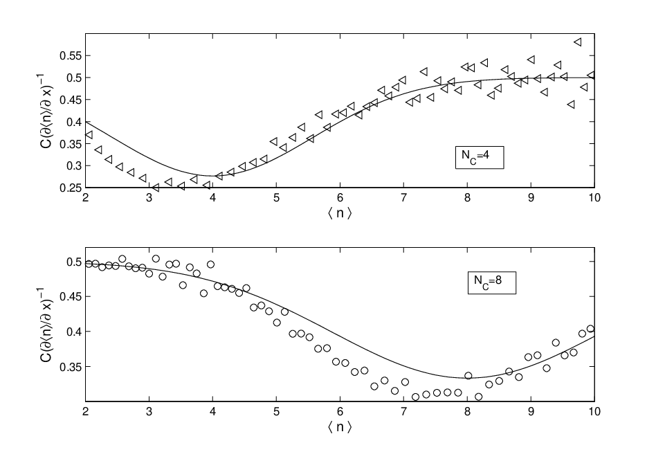
Looking at the well collapsed minima, numerical experiments confirm that the diffusivity is strictly positive: consequently, we do not expect any critical effects. More precisely, the site (i.e. the site approximately corresponding to the density ) does not give rise to any singularities in the observables describing the system. Further evidences are given in the next sections.
V.2 Poissonian
We study now the probability distribution for the particle population in the presence of a gradient. As proved in Section III, for a closed system the occupation number is a stochastic variable described by a Poissonian distribution. For an open system with a steady particle flow, the average occupation number is site dependent and its distribution is no more rigorously described by such a Poissonian. However, we expect that the differences between the exact distribution and is small when the size is large with respect to the particle gradient . We also expect that, the farthest from , the better the approximation works. Indeed, these facts are confirmed by numerical simulations. For example, in Fig. 3 we show the probability distributions for the occupation number relevant to several sites of an open system of size , with and . Each site considered (depicted in a different colour) corresponds to an average occupation number , and the pertaining distribution is compared with the Poissonian of average , i.e. the distribution for a close system made up of particles. As expected, near the borders the two distributions perfectly overlap; in general, their difference is small away from (which is about , as pointed out in the inset). Otherwise stated, the difference is appreciable in a region around . Moreover, experiments show that such a region sensibly shrinks as the size gets larger.

V.3 Fluctuations
Let us study the occupation number and its fluctuations as functions of the system parameters . The interest in this point depends on the possibility, for interacting systems, of an increase in fluctuations induced by the presence of a gradient, as found e.g. in [11, 19]. More precisely, the system considered in [11] was an Ising model on a cylindrical lattice, in contact with two thermostats at temperatures and . In the presence of a heat flow (), it was found that fluctuations (generically denoted as ) relevant to several observables all satisfy the following
where and represent the fluctuations in the system with and without flow, respectively. Moreover, such difference is especially important in a domain of energies around , the critical energy of the Ising system at equilibrium.
Clearly, analogous comparisons can be carried out for our RW model, by considering fluctuations in the occupation number for open steady systems in the absence () or presence () of a particle flow. Notice that, apart from negligible border effects, the former case is well described by the close system of Section III where the exact value of the fluctuations can be evaluated from the Poissonian distribution (i.e. ), allowing for an accurate insight into the problem.


Figures 4 and 5 show as a function of for different choices of the system parameters. Actually, when a steady particle flow is established, (i) , (ii) at a density deviations from the equilibrium values are stronger, and (iii) the overall effect is more significant in a region . The analogy with the Ising system is notable.
Figures 4 and 5 also highlight the role of the size and of the density gradient: by enlarging or by reducing , the region gets smaller and the discrepancy shrinks. Again, this effect is consistent with the results found for the ferromagnetic model undergoing a steady heat flow.
Thus, both the ferromagnetic and the RW systems exhibit an increase in fluctuations when a gradient is established. However, such a gradient is not a sufficient cause: sites have to interact so that a dynamical slowing down takes place for a value of the parameter (energy and particle density respectively). For the Ising model, such a special value of the energy corresponds to the critical point. As for RW, it is the parameter in the interaction defined by Eq. 19.
Now, Ising and RW systems display an important difference: while for the former exhibits a true critical point, the latter is never critical, since does not correspond to any singular behaviour. In particular, (to be related to the diffusivity) is always finite.
We can conclude that the similar increase in fluctuations, observed in both systems, is not really due to criticality but only to a dynamical slowing down. This solves the apparent contrast remarked in the Ising case between the mesoscopic nature of the effect and the thermodynamic nature of the critical point.
V.4 Scaling
Previous observations can be stressed by looking directly at the scaling behaviour. In general, as well known, fluctuations are sensitive to criticality. The functional dependence on the size , for instance, is different at the critical point. This happened indeed in the Ising model at [11]. Now, since in the present case is not a genuine critical point, as grows we expect, conversely, a regular behaviour for all occupation numbers, those approaching included. Such an expectation is confirmed by experiments reported in Figure 6, where goes to zero as gets larger according to the scaling law: , with an excellent data collapse. The only relevant effect appearing at regards the amplitude of , which has a maximum, not a distinct scaling law.

V.5 Spectral features
Time series can provide further information on the pseudo criticality around
. It is worth summarizing how this kind of analysis is performed.
For a given site , consider the sequence of occupation numbers:
where are instants of time after the onset of a steady state. This definition may be implemented by introducing a time delay , and the corresponding time series:
Clearly, the delay or sampling parameter plays an important role in experiments, since time correlations are strong in our model, and a sufficiently long interval is needed before a given configuration significantly changes.
Then, by Fast Fourier Transform, from time series we get power spectra , i.e. the square of absolute Fourier transform amplitudes in the frequency domain. The so-called colour exponent describes the possible power-law decay of the spectrum. It can be obtained as the angular coefficient of the linear fit in the log-log plot of vs. .
Of course, a special value is associated to white noise, decorrelation, randomness. Values qualify coloured noises corresponding to different types of temporal correlations. In particular, (“pink” or noise) implies an extremely slow decay of correlations.
As it is well known, a general dynamic theory of coloured noise is still lacking (see however [20]). The old suggestion of Van der Ziegle, getting noise from the superposition of independent Poisson processes [21, 22], could be of some interest in our case.
In simulations, for every , exponents are evaluated and averaged over several runs starting from different initial conditions, up to stabilization. The dependence of the noise on interaction is shown in Fig. 7, where exponents versus are plotted for analogous systems made up of interacting and non-interacting (i.e. isotropically diffusing) particles; several choices of are also considered. Systems of larger sizes, not reported here, display qualitatively alike outlines.

The presence of interaction clearly shifts towards
smaller values, but only in a domain around largely overlapping
the previously considered domain .
Indeed, is minimum for . This
confirms that around correlations are stronger and the
dynamics is slowed down. Moreover, the comparison with the
non-interacting system allows to figure out the background
time-correlation which, as expected, decreases as is
larger, up to .
A less trivial point has to be underlined: the difference between
interacting and non-interacting case is not a monotonic function
of and, therefore, neither of itself.
Actually, there exists an optimal time delay
maximizing the effect of interaction over time correlation.
Such a special delay seems difficult to be
interpreted, and could suggest that there exist further
aspects, besides the superposition of
Poisson processes, characterizing the noise in our model.
VI Conclusions and perspectives
We have introduced a system of interacting random walkers modelling several situations where diffusivity depends on the density of the diffusing entities. Our model constitutes a special case of misanthrope processes, characterized by a totalistic hopping amplitude. We have shown analytically that the equilibrium distribution is factorized into a product of Poissonian functions.
Despite a simple equilibrium behaviour, far from equilibrium the study of the system presents some non-trivial tasks. Indeed, in principle, local properties such as correlations and factorizability are deeply influenced by non equilibrium. In our case, we succesfully explored the reliability of a perturbative approach to the problem. Since, on one hand, the equilibrium properties are analytically known and, on the other, interaction still plays a relevant role, our model can be considered as an interesting benchmark for the study of non-equilibrium effects. By recovering analogous results in magnetic models, we have clarified some open problems, concluding, in particular, that a density dependent diffusivity and the presence of a dynamical slowing down are necessary premises to the amplification of fluctuations, while, on the contrary, the existence of a true critical point may cooperate but it is not strictly necessary.
Finally, even if the passage to regular lattices of higher dimensionality does not present any substantial novelty, we evidenced a possible deep interplay between time scaling, substrate topology and local interactions. Consequently, there still exist in this context a number of geometro-dynamical aspects which have to be developed, understood and classified. The non trivial influence of interaction on the noise can be considered as a notable hint for the relevance of the matter.
References
- [1] H. Mehrer, Diffusion in Solids: Fundamentals, Methods, Materials, Diffusion-Controlled Processes, Springer Series in Solid-State Sciences, Berlin 2007.
- [2] J. Kärger, F. Grinberg and P. Heitjans, Diffusion Fundamentals, Leipziger Universitätsverlag, Leipzig 2005.
- [3] S. Lepri, R. Livi and A. Politi, Phys. Rep. 377, 1 (2003).
- [4] M. Marinelli, F. Mercuri, U. Zammit, R. Pizzoferrato F. Scudieri, D. Dadarlat, Phys. Rev. B 49, 4356 (1994).
- [5] A. Pawlak, Phys. Rev. B 68, 094416 (2003).
- [6] G. Flierl, D. Grünbaum, S. Levin and D. Olson, J. Theor. Bio. 196, 397 (1999)
- [7] N.G. van Kampen, Stochastic Processes in Physics and Chemistry, North-Holland Personal Library, Oxford 1997.
- [8] R. Harris and M. Grant, Phys. Rev. B 38, 9323 (1988).
- [9] K Saito, S. Takesue and S. Miyashita, Phys. Rev. E 59, 2783 (1999).
- [10] M. Casartelli, N. Macellari and A. Vezzani, Eur. Phys. J. B 56, 149 (2007).
- [11] E. Agliari, M. Casartelli and A. Vezzani, Eur. Phys. J. B 60, 499 (2007).
- [12] G.H. Weiss, Aspects and Applications of the Random Walk, North-Holland, Amsterdam 1994.
- [13] M. R. Evans and T. Hanney, J. Phys. A: Math. Gen. 38, R195 (2005).
- [14] G.M. Schütz, Exactly Solvable Models for Many-Body Systems Far From Equilibrium, in Phase Transitions and Critical Phenomena 19, 1 - 251, C. Domb and J. Lebowitz eds., Academic Press, London 2000.
- [15] B. Derrida, J.L. Lebowitz and E.R. Speer, Phys. Rev. Lett. 87, 150601 (2001)
- [16] B. Derrida, B. Ducot and P.E. Roche J. Stat. Phys. 115, 717 (2004)
- [17] R.J. Harris, A. Rákos and G.M. Schutz J. Stat. Mech. P08003 (2005)
- [18] T. Bodineau and B Derrida, cond-mat arXiv:07042726 (2007)
- [19] A. Dhar and D. Dhar, Phys. Rev. Lett. 82, 480 (1999).
- [20] M.B. Weissman, Rev. Mod. Phys. 60, 537 (1988).
- [21] A. Van der Ziegle, Physica 16, 359 (1950).
- [22] H. J. Jensen, Self-Organized Criticality, Cambridge University Press, Cambridge 1998.