A Perturbative Approach to Inelastic Collisions in a Bose-Einstein Condensate

A Bose-Einstein condensate (BEC) is a state of matter in which a large number of bosons occupy the same quantum mechanical ground state. As such, BECs present the opportunity to study quantum systems which display large scale (macroscopic) collective behaviour. Recently there has been much interest in multi-component BECs because of their importance to quantum optics [1, 2, 3, 4]. Multi-component BECs are most often formed in a multi-well potential in which the components are spatially separated [2, 4]. Alternatively, the multi-component formalism can be used to model a single component BEC that possesses several internal degrees of freedom, such as varying amounts of spin [3].

In general, many-body systems are of significant importance in physics. For example, quantum information processes require the manipulation and control of systems with large numbers of particles. However, many-body systems are often difficult to treat exactly and are most often studied using numerical or approximate methods. The realm of applicability of these methods is limited by the number of degrees of freedom of the system. Two common approximate models are the Bose-Hubbard model of quantum optics [4] and closely related to it, the Lipkin-Meshkov-Glick model of nuclear physics [5], both used to describe the two-body interactions of spin-$J$ systems.

A family of exactly solvable many-body systems was introduced in [6] and studied in greater depth in [7]. These models can be used to describe the physics of a two component BEC where both elastic and mode-exchange inelastic collisions are present. Mode-exchange collisions are known as general nearest neighbor interactions in the context of multi-well BECs [9] and as inelastic collisions in the case of a single condensate consisting of particles in two hyperfine levels [10]. The family of models is parameterized by a positive integer $n$, and hence the specific models are called $n$-models. This terminology is used because the $n$-model contains $1,2,\dots,n-$body interactions. Analytic solutions can be found for the $n$-model when the strengths of the various particle interactions obey specific constraints. While the $n$-models are of interest to many-body physics in general, in this paper we will largely be concerned with the $2$-model where only single body interactions and two-body collisions are considered. Microscopic calculations show that mode-exchange collisions occur in BECs as a result of the interaction of a laser field with the system [10]. The 2-model includes the usual Josephson-type interactions, but also allows the effects of mode-exchange collisions to be studied analytically, and as such provides a more realistic framework for studying two-mode BECs than the canonical Josephson Hamiltonian [11].

The analytic solution found in [6] requires that the strengths of the various interactions meet certain constraints; if these constraints are not met the solution is invalid. While in some experimental situations the rates of inelastic and elastic mode-exchange collisions can be controlled externally [12], this is not always the case. Moreover, even in if the rate of collisions can be manipulated, the constraints will likely still only be approximately satisfied. It is thus of interest to extend the solution space of the system to the case in which these constraints are only approximately satisfied. This naturally leads to the consideration of small parameter perturbations in the model to study its robustness. Along with perturbations within the model it is of interest to include additional interaction terms as perturbations, such as inelastic collisions resulting in particle loss. Particle loss, often suppressed in experimental settings, is studied theoretically by considering classical rate equations [11]. More recently, a quantum treatment of 3-body loss has been given in [13]. Including external perturbations extends the predictive power of the model. Additional interactions of primary interest include three-body recombination, background collisions, spin exchange and dipole relaxation [11]. To our knowledge, this is the first study which analyzes particle loss as a perturbative effect in BECs.

Motivated by the above considerations, in this paper we carry out a full perturbative analysis of the solvable BEC 2-model proposed in [6]. We begin by reviewing this model and the solutions derived when the constraint equations on the parameters are satisfied [7]. We then introduce perturbations to the parameters in the model and analyze the effects on the particle distribution, entanglement and the evolution of the relative number operator. In later sections we discuss the effects of state degeneracy and the inclusion of a general loss term as a perturbation, illustrating the formalism by studying background collisions and three-body recombination.

The $2$-model studied in [6, 7] is governed by the Hamiltonian

where $h.c.$ denotes the Hermitian conjugate of the preceding term. The two modes $a$ and $b$ are independent Bose operators satisfying $[a,a^{\dagger}]=1=[b,b^{\dagger}]$ with the commutators of all remaining pairs vanishing. The term $\omega\left(a^{\dagger}a-b^{\dagger}b\right)$ is the free energy of $\hat{n}_{a}=a^{\dagger}a$ particles in the $a$ mode and $\hat{n}_{b}=b^{\dagger}b$ particles in the $b$ mode, with frequency difference $\omega$ between modes. This frequency difference arises because the model describes atoms in different hyperfine levels, or alternatively unsymmetric spatially separated condensates [14]. A Josephson-type or spin flip interaction is included with strength $\lambda$ and phase $\phi$. In practice such an interaction is induced by an external field, such as a laser [8]. This interaction may also be interpreted as modeling the tunneling of particles between modes with probability proportional to $\lambda$. Also included are terms corresponding to number-preserving elastic and mode-exchange collisions, namely those terms containing four bose operators. The interaction with strength $\mu$ is a single dispersive process. The interaction with strength $\Lambda$ describes a collision where two particles exchange their mode. The elastic interaction has strength $\mathcal{U}$ and models the collision of a particle from each mode in which the number of particles in each mode is conserved. We see that the mode-exchange collisions preserve the total particle number but not the relative particle number.

The Hamiltonian given in eq. (1) can be efficaciously studied by first introducing the simpler Hamiltonian [6]

with real constants $A_{1}$ and $A_{2}$. Such a Hamiltonian models a two-mode condensate with energy difference $A_{1}$ between modes and elastic scattering probability proportional to $A_{2}$. As is clear from the form of $H_{0}$ the relative number operator $\hat{m}=a^{\dagger}a-b^{\dagger}b$ is a commuting observable so that the number of particles in each mode is conserved. In particular, there is no probability of spin-flip or tunneling between modes. We also note that the total number operator $\hat{N}=a^{\dagger}a+b^{\dagger}b$ commutes with $H_{0}$. We may thus take the eigenvalues $N$ and $m$ of $\hat{N}$ and $\hat{m}$ as labels of the eigenstates, for which we write $|N,m\rangle$. For fixed $N\in\mathbb{N}$ the values of $m$ are limited to¹¹ 1 See the appendix for details. $-N,-N+2,\dots,N-2$ and $N$. The energy of the state $|N,m\rangle$ is $E_{m}=A_{1}m+A_{2}m^{2}$.

For a certain choice of parameters in $H_{2}$ the solutions $|N,m\rangle$ of $H_{0}$ can be used to obtain analytic solutions of $H_{2}$. To see this, define a two-mode displacement operator by $U\left(\xi\right)=\exp\left(\xi a^{\dagger}b-\xi^{*}ab^{\dagger}\right)$ with displacement parameter $\xi=\frac{1}{2}\theta e^{i\phi}$. It is clear that $U\left(\xi\right)$ is unitary. It can then be shown that if the parameters in $H_{2}$ satisfy

then $H_{2}=U^{\dagger}H_{0}U$, a result shown by computing

Observe that $U\left(\begin{array}[]{cccc}a&b&a^{\dagger}&b^{\dagger}\\ \end{array}\right)^{T}U^{\dagger}$ may be computed by setting $\theta\mapsto-\theta$ in eq. (4).

Since the eigenvectors of $H_{0}$ are of the form $|N,m\rangle$ the eigenvectors of $H_{2}$ when satisfying eqs. (3) are simply $U^{\dagger}|N,m\rangle$ with energy $E_{m}=A_{1}m+A_{1}m^{2}$. An extensive analysis and discussion of these solutions is included in [7].

For fixed $N\in\mathbb{N}$ the ground state of $H_{2}$, labeled as $|\psi_{m_{0}}\rangle=U^{\dagger}|N,m_{0}\rangle$, is found by minimizing the energy $E_{m}=A_{1}m+A_{2}m^{2}$ with respect to $m$. First assume $A_{2}<0$. In this case, if $A_{1}<0$ ($A_{1}>0$) the minimum occurs at $m_{0}=N$ ($m_{0}=-N$). Secondly, say $A_{2}>0$. If $\left|\frac{A_{1}}{2A_{2}}\right|\leq N$, then $m_{0}$ is the closest allowable²² 2 The integer $m$ can only take the values $-N,-N+2,\dots,N-2$ and $N$; see the appendix for details. integer to $-\frac{A_{1}}{2A_{2}}$; otherwise $m_{0}$ is the closest allowable integer to $-\hbox{sgn}(A_{1})N$. In particular, a choice of either $m_{0}$ or $\frac{A_{1}}{A_{2}}$ determines the other.³³ 3 In calculations we will assume $A_{2}=1$, so that a choice of $m_{0}$ determines $A_{1}$.

It is important to recall that, in the case of a double-well BEC, the two-mode approximation must be satisfied [1]. This means that collisions taking place in the region where the wavefunctions overlap must be less probable than collisions between particles belonging to the same well. It is possible to find an exact analytic solution to the model in this case by considering $\theta<<1$. It is interesting to observe that it is not possible to find analytical solutions to this model for an exactly symmetric double-well and satisfy, simultaneously, the two mode approximation. Fortunately, in the case of slightly asymmetric double wells (which corresponds to a more realistic situation) it is possible to find exact analytical solutions in the two-mode approximation [7] .

The most general $n$-model Hamiltonian discussed in [6] has as its Hamiltonian $H_{n}=U^{\dagger}H_{0,n}U$ where $H_{0,n}=\sum_{k=1}^{n}A_{k}\hat{m}^{k}$. The eigenvectors of $H_{n}$ are again $U^{\dagger}|N,m\rangle$ with the same energy $E_{m}$. The same process of matching coefficients in the expansion of $U^{\dagger}H_{0,n}U$ that was used to obtain eqs. (3) can be carried out so that $U^{\dagger}|N,m\rangle$ is the exact solution of a Hamiltonian containing up to $n$-body interactions. In the general case, there are $n+2$ free variables (the $n$ $A_{i}$ as well as $\theta$ and $\phi$) in $UH_{0,n}U^{\dagger}$, whereas the number of terms in a general Hamiltonian describing such interactions is $(n+2)(n+4)(n+6)/48$ as shown in Appendix B. So while the above method continues to give analytic solutions for all $n$, its range of applicability decreases as $n$ grows. It should also be noted that because $H_{0,n}$ contains only terms with the same number of creation and annihilation Bose operators, this formalism cannot be used to study interactions involving an odd number of Bose operators, such as the interaction $a^{\dagger}ba$ where one particle is lost.

We remark that all of the perturbative analysis carried out below is valid not only for the $2$-model, but also for the more general $n$-models. This is so because the solutions for all $n$-models are $U^{\dagger}|N,m\rangle$. We need only change the interpretation of the perturbative analysis in each case.

While satisfying eqs. (3) is sufficient to obtain an analytic solution of $H_{2}$, the method presented above fails to produce solutions if the parameters in $H_{2}$ deviate even slightly from these constraints. Thus, in order to compare this model to experimental results we would like to study the solutions to $H_{2}$ when the constraints are only approximately satisfied. We proceed with these perturbation calculations in the section below.

We begin by perturbing each of the coupling constants in $H_{2}$ away from the conditions given by eqs. (3), i.e. perturbations of the form $\omega\mapsto\omega+\delta_{\omega}$ where $\omega$ satisfies eqs. (3) and $\delta_{\omega}$ is small. We omit the study of perturbations $A_{0}\mapsto A_{0}+\delta_{A_{0}}$ since this simply leads to a shift in the energy of the state by $\delta_{A_{0}}$. In what follows, we assume that all eigenstates are non-degenerate; the degenerate case is discussed in Section 7. Throughout the paper, given an operator $\mathcal{O}$ we define $\tilde{\mathcal{O}}:=U\mathcal{O}U^{\dagger}$. To perform many of the calculations that follow we have made use of a coordinate transformation between the $\left\{N,m\right\}$ basis and the $\left\{n_{a},n_{b}\right\}$ basis, $|N,m\rangle\mapsto\left|n_{a}=\frac{N+m}{2},n_{b}=\frac{N-m}{2}\right>$ where $n_{a}$ is a eigenvalue of $\hat{n}_{a}=a^{\dagger}a$ and similarly for $n_{b}$.

In the unperturbed case we can use the analytic solution $|\psi_{m_{0}}\rangle=U^{\dagger}|N,m_{0}\rangle$ for parameters satisfying eqs. (3) to find an explicit expression for the particle distribution:

Using the homomorphism described in the appendix to relate the Schwinger $\mathfrak{su}(2)$ representation to the angular momentum representation we write $P=|d_{m,m_{0}}^{N}|^{2}$ where⁴⁴ 4 $d_{m,m_{0}}^{N}$ are the Wigner rotation matrix elements under the effect of the Lie algebra homomorphism discussed in the appendix. To see why these appear, observe that $U^{\dagger}=e^{-i\theta\mathbf{n}\cdot\mathbf{J}}$ where $\mathbf{n}=\left(\sin\phi,\cos\phi,0\right)$ and $\mathbf{J}=\left(\hat{J}_{x},\hat{J}_{y},\hat{J}_{z}\right)$ is the total angular momentum vector operator. That is, $U^{\dagger}$, and hence $U$, are rotations of the algebra generated by $a$ and $b$. [15]

and

The integers $k_{\pm}$ are chosen so that the arguments of the combinatorial symbols are non-negative; explicitly, $k_{-}=\hbox{max}\left\{0,\frac{m_{0}-m}{2}\right\}$ and $k_{+}=\hbox{min}\left\{\frac{N-m}{2},\frac{N+m_{0}}{2}\right\}$. We plot in Figure 1 the unperturbed particle distribution for $N=1000$, $\theta=1$ and $m_{0}=1000,\;998$ and $996$. Observe that the particle distribution is independent of phase $\phi$. We will see that this does not hold in the perturbed case. As $\theta$ varies the distributions shift along the $m$-axes; for $\theta$ small the maxima shift toward $m=N$, and move toward $m=-N$ as $\theta$ grows.

The canonical $2$-mode BEC predicts (under certain circumstances) that the ground state solution is a superposition of two peaked distributions. From Figure 1 we see that for $m_{0}<N-2$ the ground state is a superposition of more than two distributions, an effect that is due to the mode-exchange collisions not included in the canonical model [7].

In order to include perturbative effects in the particle distribution we replace the zeroth order ground state wave function $U^{\dagger}|N,m_{0}\rangle$ in eq. (18) with that including first order corrections,

Recall that in the non-degenerate case a perturbation $H^{\prime}$ induces a first order wave function correction given by

where the superscripts indicate to what order in the perturbation the term corresponds; when no superscript is present the result is to zeroth order. With this, we find that to first order the particle distribution is given by⁵⁵ 5 Throughout the rest of the paper, where appropriate, we write $\displaystyle\sum_{n=-N}^{N}$ with the understanding that we actually mean $\displaystyle\sum_{n\in\left\{-N,-N+2,\dots,N-2,N\right\}}$. Summations of this form arise because of the restriction on the eigenvalues of the relative number operator.

We show in Figures 2 - 6 the particle distributions under each of the five parameter perturbations considered above. Note that in certain cases $P^{(0+1)}$ may be negative because the first order term in eq. (22) depends linearly on the perturbation coefficients $a_{m,n}$; this of course is just a reflection that only first order corrections have been taken into account.

We see from eq. (22) and the fact that $a_{m,n}$ is proportional to the sign of the perturbation that each of the perturbations can be used to either enhance or diminish the particle distributions in the vertical direction for a given $m$. That is, given a fixed relative number $m$, by choosing the sign of the perturbation appropriately we can increase or decrease the probability of the system being in the state $|N,m\rangle$. We also see that as $|m_{0}|$ decreases the number of local maxima of the particle distribution increases, and the asymmetry of the perturbations becomes more significant, vertically diminishing probability amplitudes on one side of the central maxima while vertically stretching the amplitudes on the opposite side. The figures also show that the system is much less sensitive to perturbations in $\omega$ and $\lambda$ than it is to perturbations in the collision coupling constants; in the figures the perturbations of $\omega$ and $\lambda$ are between $7$ and $100$ times greater than those in the collision perturbations ($\Lambda,\mu$ and $\mathcal{U}$), while the corrections in all of the cases are of the same scale. Moreover, out of the collision parameters the particle distribution is most sensitive to perturbations in coupling constants of the mode-exchange collisions ($\mu$ and $\Lambda$). It is thus beneficial to maximize the matching of the mode-exchange collision constraints (3) through redefinition of parameters, allowing the perturbation to have a larger effect on the $\omega$, $\lambda$ and $\mathcal{U}$ terms.

The effect on the particle distributions of varying $\theta$ is to shift the position of the central maxima on the $m$-axis: for $\theta=\frac{\pi}{2}$, corresponding to the case in which the Josephson-type interaction is maximal ($\lambda=A_{1}$) and the energy of each mode is equal ($\omega=0$), the distribution is centered around $m=0$, while for $\theta=0$ ($\theta=\pi$), in which the Josephson-type interaction vanishes ($\lambda=0$) and the energy difference of the modes is maximal ($|\omega|=A_{1}$) it is centered $m=N$ ($m=-N$). In each of the cases, despite being centered around different values of $m$ the perturbations display the same qualitative behaviour for any choice of $\theta$. Throughout the paper we have chosen $\theta=1$ in the figures as this lies between the extremes of $\theta=0$ and $\theta=\frac{\pi}{2}$. As $\theta$ varies the effects of the perturbations vary in size, but show the same characteristics. For example, as $\theta$ decreases from $1$ to $0$ (but with $\delta$ fixed), the perturbations have a larger effect on the particle distributions, which indicates that for small values of $\theta$, we must be more careful about the size of the chosen $\delta$. This can be explained as follows. In the perturbed case the area under the particle distributions sums to unity only to first order in the perturbation. This sum is also a function of $\theta$ (since the perturbed terms are), unlike in the unperturbed case. We have found that as $\theta$ decreases the sum of probabilities decreases too, which explains why there is a difference in the particle distributions when we keep the size of the perturbations $\delta$ fixed. If we decrease both $\theta$ and $\delta$, then we find that the particle distributions essentially only shift along the $m$-axis, but not in their general shape.

Entanglement arises in many-body quantum systems because of the superposition principle and the tensor product structure of the Hilbert space⁶⁶ 6 Note that we have been using the shorthand $|N,m\rangle\equiv|n_{a}=\frac{N+m}{2}\rangle\otimes|n_{b}=\frac{N-m}{2}\rangle$., a property of utmost importance in quantum control and quantum information. In particular, states with high entanglement are desirable because of their utility in carrying out quantum information tasks [16]. We would like to determine whether or not by careful choice of the perturbations we can increase the entanglement from that of the unperturbed case.

For a bipartite quantum system the von-Neumann entropy $S=-Tr\left(\rho\log_{2}\rho\right)$ is a standard measure of the entanglement of the system, $\rho$ being the reduced density matrix. In the case at hand this reduces to

where $P$ is either the perturbed or unperturbed particle distribution, depending on the situation. As noted in the section above, the first order particle distribution given by eq. (22) can be negative for certain choices of perturbations. To resolve this problem we could either replace $P^{(0+1)}$ with $\left|P^{(0+1)}\right|$ or we could include the second order term $\left|\sum_{n=-N}^{N}a_{m_{0},n}d_{m,n}^{N}\right|^{2}$ in $P^{(0+1)}$; we use the former approach to keep the calculations strictly to first order.

When the particle distribution contains first order corrections, $P^{(0+1)}=P^{(0)}+P^{(1)}$, the entanglement is given by

For the case at hand we read off that $P^{(1)}=2d_{m,m_{0}}^{N}\sum_{n=-N}^{N}\hbox{Re}\left(a_{m_{0},n}\right)d_{m,n}^{N}$. Hence we have a criterion for increasing the entanglement of the system. Namely, we increase the entanglement (to first order) precisely when

Note that $P^{(1)}(N,m_{0},m,\theta)$ is proportional to the perturbation strengths, so that we can increase or decrease the entanglement by choosing the sign of the perturbation appropriately. Continuing, we note that for each $m$ we have $\log_{2}P^{(0)}(N,m_{0},m,\theta)+\frac{1}{\ln 2}>0$, so that to maximize the entanglement we should maximize each $P^{(1)}$. Of course, $|P^{(1)}|$ can be made arbitrarily large simply by choosing $\delta$ arbitrary large. However, we are limited in such a choice since we must keep $\delta$ small so that perturbation theory can be trusted.

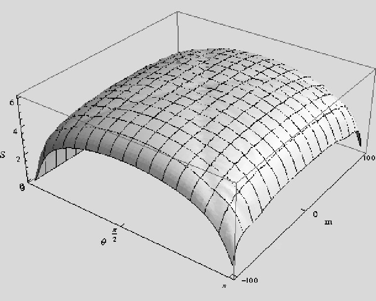
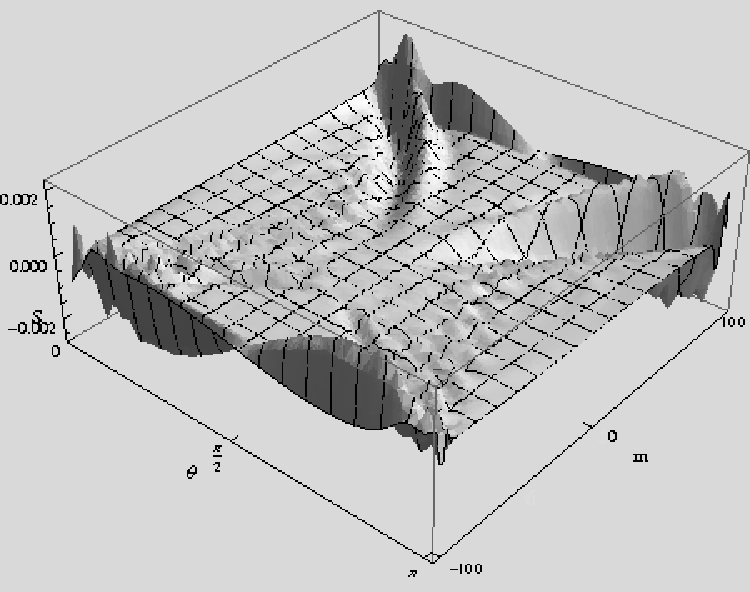
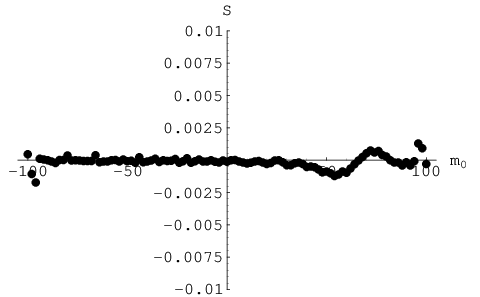
We plot in Figure 7 the unperturbed entanglement as a function of $\theta$ and $m_{0}$. See [7] for an extensive analysis. In Figures 8-12 we plot the perturbed entanglements $S^{(0+1)}$ for $\delta=0.01$ as well as the differences $\Delta S:=S^{(0+1)}-S^{(0)}$ between the perturbed and unperturbed entanglements for $\delta=0.1$; we choose a different $\delta$ in the latter case so that the differences are more evident. In each of the plots of $\Delta S$ we see that the largest changes occur approximately along the diagonal lines, connecting the points $(\theta,m_{0})=(\pi,-N)$ and $(\pi,N)$ and the points $(-\pi,-N)$ and $(\pi,N)$; these lines in $\theta-m_{0}$ space correspond to certain strengths of the coupling constants in the Hamiltonian $H_{2}$ viewed as functions of $m_{0}$. Note this type of behaviour also occurs along these lines in the unperturbed entanglement plots, as shown in Figure 7. Comparing the magnitude of the perturbative effects we observe that perturbations to the mode-exchange collision terms ($\mathcal{U},\Lambda,\mu$) have a much greater effect, their maximum difference being about an order of magnitude larger than those for $\lambda$ and $\omega$. It is also interesting to observe that the coherent states, which correspond to $U^{\dagger}|N,N\rangle$ and $U^{\dagger}|N,-N\rangle$ are the states which are maximally affected by perturbations. In such states $A_{1}$ is much larger than $A_{2}$ so that the rate of collisions is relatively small. To further study this we have plotted in Figure 13 a two-dimensional cut of Figures 8b)-12b), where we have fixed $\theta=\frac{\pi}{4}$ and allowed $m_{0}$ to vary. We observe that in each of the plots $\Delta S$ has both a local maximum and local minimum as $m_{0}$ approaches $N$.

We also observe that the most significant changes occur in the region $m_{0}>0$, where more particles lie in the $a$ mode. Positive $m_{0}$ implies that, for fixed $A_{1}>0$, the scattering length for same-mode collisions is positive and as $m_{0}$ approaches $N$, the collision rate becomes smaller. We then conclude that condensates with negative scattering lengths are more resilient to parameter perturbations and high same-mode collision rates help stabilize the condensate.

With an analytic solution to the system we may study the evolution of the relative population $\langle\hat{m}\rangle(t):=\langle\psi(t)|\hat{m}|\psi(t)\rangle$ as a function of time, where the initial state is given by $|\psi(t=0)\rangle=\sum_{m=-N}^{N}C_{m}U^{\dagger}|N,m\rangle$. For simplicity we restrict our study to the case in which $C_{m}\in\mathbb{R}$. To first order in the perturbation parameter we have

We compute $\langle\hat{m}\rangle^{(0+1)}(t)=\langle\hat{m}\rangle(t)+\langle\hat{m}\rangle^{(1)}(t)$ where

with $L_{m}:=\cos\left(\phi+\left(E_{m+2}-E_{m}\right)t\right)$ and

We plot in Figure 14 a) the unperturbed evolution of relative population given by eq. (26). We see the Rabi-like oscillations with relative population collapse and revival. In Figures 14 b) and c) we plot the evolution of relative population under the parameter perturbations $\delta_{\omega}=0.005$ and $\delta_{\omega}=0.05$, respectively. We observe that as $\delta_{\omega}$ increases the time-averaged value of $\langle\hat{m}\rangle^{(0+1)}$ decreases; from eq. (27) changing the sign of $\delta_{\omega}$ would have increased this average value. We see in Figure 14 c) that the perturbation has broken down; the maximum value of $|\langle\hat{m}\rangle^{(0+1)}|$ is greater than the total particle number. This breakdown reminds us that we must not let the perturbation grow too large for our analysis to be reliable. We also see (in Figure 14 c) that as $\delta_{\omega}$ grows the time of population collapse significantly decreases. Because of the complexity of the correction term eq. (27) an analytic study of the effects of the perturbations on population collapse and revival times is not possible.

¿From eq. (26) we see that in the unperturbed case an initially pure state remains pure. Eq. (27) shows that the same holds true even in the perturbed cases. Hence, $\langle\hat{m}\rangle^{(0+1)}(t)$ has non-trivial time-dependence if and only if the initial state is entangled.

Throughout the above analysis we have assumed that the unperturbed states in question are non-degenerate. We proceed now to study the degenerate case, which results for specific values of the constants $A_{1}$ and $A_{2}$. For fixed total particle number $N$ two distinct states, labeled by relative population numbers $m_{1}$ and $m_{2}$, have the same energy precisely when $m_{1}+m_{2}=-\frac{A_{1}}{A_{2}}$. From the analysis of the perturbations completed above we know that the perturbation matrix elements are non-vanishing only if $m_{1}-m_{2}\in\left\{2,4\right\}$, where we have assumed without loss of generality that $m_{1}>m_{2}$. Combining these two observations we see that there are at most two pairs of degenerate states.

Let us consider as an example the perturbation $\omega\mapsto\omega+\delta_{\omega}$ with $A_{1}=-\left[N+(N-2)\right]A_{2}$, so that the only pair of degenerate states is $|N,N\rangle$ and $|N,N-2\rangle$; each have energy $A_{2}N\left(2-N\right)$. The matrix of interest is

its eigenvalues and eigenvectors yield the first-order energy and wave function corrections. Using the calculations performed above it remains to find the solutions $\epsilon_{\pm}$ of the quadratic $\hbox{det}\left(\Delta_{\omega}-\epsilon I_{2\times 2}\right)=0$. The eigenvalues (energy corrections) and corresponding eigenvectors (wave function corrections) of $\Delta_{\omega}$ are

with $a_{\pm}$ a suitable normalization constant.

Figure 15 a) plots $\epsilon_{\pm}$ as a function of $\theta$ for $N=1000$ and $\delta_{\omega}=0.01$. We see that the energy is lowered for all values of $\theta$; had $\delta_{\omega}$ been negative the opposite would have been true. We see from Figures 15 b) and c), which plot the perturbed particle distributions for $\delta_{\omega}=\pm 0.01$, that even for very small perturbations in $\omega$ there is a noticeable change in the particle distribution. This is in contrast to the non-degenerate perturbation of $\omega$, where even for $\delta_{\omega}=15$ there was not a large change in the particle distribution. The induced change in the particle distribution is also qualitatively different from that in the non-degenerate case. This arises because the correction in the degenerate case is sinusoidal with frequency much greater than that of the unperturbed particle distribution. Regardless of the sign of $\delta_{\omega}$ we see that the central maximum of the particle distributions is shifted to smaller values of $m$.

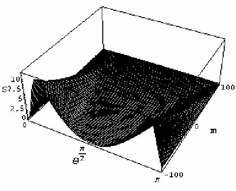
We plot in Figure 16 a) the perturbed entanglement as a function of $\theta$ and $m_{0}$ for $\delta_{\omega}=0.005$ and $N=100$, while b) of the same figure plots the difference $\Delta S$ for the same configuration. Even for a small perturbation strength $\delta_{\omega}=0.005$ the perturbation to the entanglement is still significant, again showing that a degenerate system is more sensitive to perturbations than is the non-degenerate case. We also observe that the largest perturbations are present for $m_{0}$ close to $-N$ and $\theta\approx\frac{\pi}{4},\frac{3\pi}{4}$. For $m_{0}$ close to $N$, the perturbations become negligible, regardless of $\theta$. Therefore, we find that high collision rates also help stabilize the condensate against perturbations in the degenerate case. However, in this case, condensates with positive scattering lengths are more stable.

Similarly, we find that for a perturbation $\lambda\mapsto\lambda+\delta_{\lambda}$, assuming again that $|N,N\rangle$ and $|N,N-2\rangle$ are the degenerate states, the energy corrections are

which is just the energy correction equation for perturbations in $\omega$ with the substitution $\cos\theta\mapsto\sin\theta$; we obtain the wavefunction corrections $|\pm\rangle$ for $\delta_{\lambda}$ in the same manner. Figure 17 plots the perturbed energy and perturbed particle distributions for $\delta_{\lambda}=1$ and $\delta_{\lambda}=\pm 0.01$. The same comments made above about Figure 15 for perturbations $\delta_{\omega}$ hold in this case as well. In Figure 18 we plot the perturbed entanglement and entanglement difference $\Delta S$ for $\delta_{\lambda}=0.005$. The figure shows similar behaviour to Figure 16. However, we note that in the case of $\lambda$ perturbations $\Delta S$ is strictly positive (for positive $\delta_{\lambda}$). There are again extrema (this time both maxima) for $m_{0}=-N$ and $\theta\approx\frac{\pi}{4},\frac{3\pi}{4}$, with $\Delta S$ vanishing as $m_{0}$ approaches $N$. Also as in the case above, the system is very sensitive to perturbations, with $\Delta S\approx 10$ at some points.

The study of degenerate perturbations in the remaining parameters is completed in the same way as is done above, so we omit these. Note that high collision rates help stabilize the condensate against perturbations in $\lambda$ for both positive and negative scattering lengths.

As mentioned in the introduction it is of interest to study perturbations that model additional interaction terms not included in the original Hamiltonian eq. (1). We will largely be interested in perturbations that do not preserve the total number of particles in the system. We begin with a general discussion of loss terms and proceed to use this formalism to discuss the effects of background collisions and three-body recombination.

References

- [1] G. J. Milburn, J. Corney, E. M. Wright, and D. F. Walls, Phys. Rev. A 55, 4318 (1997); J. I. Cirac, M. Lewenstein, K. Molmer, and P. Zoller, Phys. Rev. A 57, 1208 (1998); A. J. Leggett, Rev. Mod. Phys. 73, 307356 (2001).
- [2] M. Albiez et al. Phys. Rev. Lett. 95, 200401 (2005).
- [3] L. Santos and T. Pfau. Phys. Rev. Lett. 96, 190404 (2006); T. Ohmi and K. Machida, J. Phys.Soc. Jpn. 67, 1822 (1998); C. K. Law, H. Pu, and N. P. Bigelow, Phys. Rev. Lett. 81, 5257 (1998);M. Koashi and M. Ueda, Phys. Rev. Lett. 84, 1066 (2000); O. E. Mstercaploglu et al, Phys. Rev. A 68, 063616 (2003).
- [4] E. M. Graefe, H. J. Korsch, D. Witthaut, Phys. Rev. A 73, 013617 (2006).
- [5] H. J. Lipkin, N. Meshkov, and A. J. Glick, Nucl. Phys. 62, 188 (1965).
- [6] P. Barberis-Blostein and I. Fuentes-Schuller. J. Phys. A: Math. Theor. 40 F601 (2007).
- [7] P. Barberis-Blostein and I. Fuentes-Schuller. Phys. Rev. A 78, 013641 (2008).
- [8] C.J. Myatt et al. Phys. Rev. Lett. 78, 586 (1997).
- [9] H. Heiselberg, Phys. Rev. A, 73, 013628 (2006).
- [10] P. S. Julienne, J. Res. Natl. Inst. Stand. Technol. 101, 487 (1996); R. Napolitano, J. Weiner, and P.S. Julienne, Phys. Rev. A 55, 1191 (1997).
- [11] E. Cornell, J. Ensher and C. Wieman. cond-mat/9903109 (1999).
- [12] J.L. Roberts, N.R. Claussen, S.L. Cornish and C.E. Wie- man, Phys. Rev. Lett. 85, 782 (2000).
- [13] A. A. Norrie, R. J. Ballagh, and C. W. Gardiner, Phys. Rev. A. 73 043618 (2006); S. Wuster et.al, Phys. Rev. A 75, 043611 (2007).
- [14] J. Stenger et al. Nature. 396, 345 (1998).
- [15] K. Gottfried and T.-M. Yan. Quantum Mechanics: Fundamentals. Springer, New York, N.Y., 2004.
- [16] M. Nielson and I. Chuang. Quantum Computation and Quantum Information. Cambridge University Press, Cambridge, U.K., 2000.
- [17] M. Holzmann, W. Krauth and M. Naraschewski. Phys. Rev. A. 59, 2956 (1999).
- [18] J. Stamper-Kurn et al. Phys. Rev. Lett. 80, 2027 (1998).
- [19] C. Sackett, J. Gerton, M. Welling and R. Hulet. Atomic Physics 16: Proceedings of the Sixteenth International Conference on Atomic Physics. American Institute of Physics Conference Proceedings #477, New York, 1999. Eds. Baylis, W. and Drake, G.
- [20] J. Söding et al. Appl. Phys. B. 69, 257 (1999).
- [21] J. Schwinger. Quantum Theory of Angular Momentum. Eds. Biedenharn, L.C. and Van Dam, H. Academic Press, New York, N.Y., 1965.