Polymer quantization, singularity resolution and
the potential
Gabor Kunstatter†,
Jorma Louko♯
and
Jonathan Ziprick‡
†
Department of Physics and Winnipeg Institute of
Theoretical Physics,
University of Winnipeg
Winnipeg, Manitoba, Canada R3B 2E9
[e-mail: g.kunstatter@uwinnipeg.ca]
♯
School of Mathematical Sciences,
University of Nottingham
Nottingham NG7 2RD, United Kingdom
[e-mail: jorma.louko@nottingham.ac.uk]
†
Department of Physics and Astronomy, University of Manitoba
Winnipeg, Manitoba, Canada R3T 2N2
[e-mail: j.ziprick-ra@uwinnipeg.ca]
Abstract
We present a polymer quantization of the potential on the positive real line and compute numerically the bound state eigenenergies in terms of the dimensionless coupling constant . The singularity at the origin is handled in two ways: first, by regularizing the potential and adopting either symmetric or antisymmetric boundary conditions; second, by keeping the potential unregularized but allowing the singularity to be balanced by an antisymmetric boundary condition. The results are compared to the semiclassical limit of the polymer theory and to the conventional Schrödinger quantization on . The various quantization schemes are in excellent agreement for the highly excited states but differ for the low-lying states, and the polymer spectrum is bounded below even when the Schrödinger spectrum is not. We find as expected that for the antisymmetric boundary condition the regularization of the potential is redundant: the polymer quantum theory is well defined even with the unregularized potential and the regularization of the potential does not significantly affect the spectrum.
Revised December 2008
Published in Phys. Rev. A 79, 032104 (2009)
1 Introduction
One of the most important outcomes expected of a successful theory of quantum gravity is a clear and unambiguous solution to the problems associated with the curvature singularities that are predicted by classical general relativity. This expectation is natural since quantum mechanics is known to cure classical singularities in other contexts, such as the hydrogen atom.
In recent years there has been much work suggesting that Loop Quantum Gravity (LQG) [1] may indeed resolve gravitational singularities at least in the case of symmetry-reduced models, such as spatially homogeneous [2] and inhomogeneous [3] cosmologies and spherically symmetric black holes [4, 5, 6]. Given the simplifications that these models entail, it is pertinent to ask which features of the LQG quantization scheme are crucial to the observed singularity resolution.
There are two distinct, but related, features of the LQG quantization program that appear to play a role in achieving singularity resolution. The first is the fundamental discreteness that underlies LQG due to its focus on holonomies of connections and associated graphs embedded in a spatial manifold [7]. An analogous approach in a purely quantum mechanical context is so-called polymer quantization [8, 9], in which the Hamiltonian dynamics occurs on a discrete spatial lattice and the basic observables are the operators associated with location on the lattice and translation between lattice points. Polymer quantization provides a quantization scheme that is mathematically and physically distinct from Schrödinger quantization.
The second apparently key ingredient in the LQG singularity resolution mechanism is the regularization of the singular terms in the Hamiltonian using a trick first introduced in this context by Thiemann [7]. The regularization is achieved by first writing a classical inverse triad as the (singular) Poisson bracket of classical phase space functions whose quantum counterparts are known, and then defining the inverse triad operator as the commutator of these quantum counterparts. When applied to simple models this procedure gives rise to quantum operators with bounded spectra. The singularity is therefore kinematically “removed” from the spectra of relevant physical operators, such as the inverse scale factor.
One question that arises concerns the role or perhaps the necessity of the Thiemann trick in singularity resolution in LQG. Recall that in the case of the hydrogen atom the singularity resolution is achieved by defining self-adjoint operators in a Hilbert space. This requires a careful choice of boundary conditions on the wave function [10] but does not require modification of the singular potential. An example more relevant to quantum gravity is the reduced Schrödinger quantization of the “throat dynamics” of the Schwarzschild interior, which on imposition of suitable boundary conditions produced a discrete, bounded-from-below spectrum for the black hole mass [11].
Polymer quantization of the hydrogen atom was recently examined in [12], retaining only the s-wave sector and regularizing the potential in a way that lets take values on the whole real axis. The choice of symmetric versus antisymmetric boundary conditions at the singularity was found to have a signficant effect on the ground state even after the singularity itself had been regularized. In particular, in the limit of small lattice separation the ground state eigenenergy showed evidence of convergence towards the ground state energy of the conventionally-quantized Schrödinger theory only for the antisymmetric boundary condition.
In the present paper, we perform a similar polymer quantization of the more singular potential. When the potential is regularized, we shall find that the choice of the boundary condition again has a significant effect on the lowest-lying eigenenergies. However, we shall also find that the polymer theory with the antisymmetric boundary condition is well defined even without regularizing the potential, and with this boundary condition the regularized and unregularized potentials yield closely similar spectra. The boundary condition at the singularity is hence not only a central piece of input in polymer quantization, but it can even provide, along with the modification to the kinetic term, the pivotal singularity avoidance mechanism. While this is expected from general arguments that we will make explicit later on, it is interesting and reassuring to see the mechanism work in the special case of the potential, whose degree of divergence is just at the threshold where a conventional Schrödinger quantization will necessarily result into a spectrum that is unbounded below. The polymer treatment of this system is thus turning a Hamiltonian that is unbounded below into one that has a well-defined ground state.
The potential is interesting in its own right: it has a classical scale invariance that is broken by the quantum theory. In addition, this potential appears frequently in black hole physics, for example in the near horizon and near singularity behaviour of the quasinormal mode potential [13, 14], in the near horizon behaviour of scalar field propagation [15] and in the Hamiltonian constraint in Painlevé-Gullstrand coordinates [16]. It may therefore conceivably be of direct relevance to quantum gravity. There is a substantial literature on Schrödinger quantization of this potential in (see for example [17, 18, 19, 20, 21, 22, 23] and the references in [24]), but we are not aware of previous work on polymer quantization of this potential.
Our paper is organized as follows. In Section 2 we review the Schrödinger quantization of the porential in . In Section 3 we formulate the polymer quantization of this system on a lattice of fixed size and describe the numerical method. We also include in this section a computation of the semi-classical polymer spectrum from the Bohr-Sommerfeld quantization condition, with a fixed polymerization length scale. The numerical results are presented in Section 4 and the conclusions are collected in Section 5.
2 Schrödinger quantization
We consider the classical Hamiltonian
| (2.1) |
where the phase space is with and is a constant. We shall take , and all dimensionless, and on quantization we set . If physical dimensions are restored, and will become expressed in terms of a single dimensionful scale but remains dimensionless. That the coupling constant is dimensionless is the speciality of a scale invariant potential.
Quantization of (2.1) is of course subject to the usual ambiguities. In particular, if one views as an effective Hamiltonian that comes from a higher-dimensional configuration space via symmetry reduction, with being a radial configuration variable, the appropriate Hilbert space may be , where is a positive-valued weight function. If for example , where , then the ordering
| (2.2) |
makes the quantum Hamiltonian symmetric. If the wave function in is denoted by , we may map to by , and is then mapped in to the Hamiltonian
| (2.3) |
where
| (2.4) |
We shall consider any such mappings to have been done and take the quantum Hamiltonian to be simply
| (2.5) |
acting in the Hilbert space .
To guarantee that the time evolution generated by (2.5) is unitary, must be specified as a self-adjoint operator on [25]. A comprehensive analysis of how to do this was given in [19] (see also [17, 18, 20, 21, 22, 23]). We shall review the results of [19] in a way that displays the spectrum explicitly for all the qualitatively different ranges of .
Before proceeding, we mention that several recent quantizations of the potential first regularize the potential using various renormalization techniques [20, 21, 22]. In particular, when the spectrum of a self-adjoint extension is unbounded below, these renormalization techniques need not lead to an equivalent quantum theory [23]. We shall here discuss only the self-adjoint extensions.
To begin, recall [25] that the deficiency indices of are found by considering normalizable solutions to the eigenvalue equation . An elementary analysis shows that is essentially self-adjoint for , but for a boundary condition at is needed to make self-adjoint. Physically, this boundary condition will ensure that no probability is flowing in/out at .
2.1
For , we write with .
For , the linearly independent (non-normalizable) solutions to the eigenvalue equation
| (2.6) |
are . These oscillate infinitely many times as . To find the boundary condition, we consider the linear combinations
| (2.7) |
where is a parameter that a priori could depend on . As is periodic in with period , and as replacing by multiplies by , we may understand periodic with period . For concreteness, we could choose for example .
For the probability flux through to vanish, we need
| (2.8) |
for all and , where the overline denotes the complex conjugate. Using the small argument asymptotic form (equation (9.1.7) in [26])
| (2.9) |
this is seen to require , and hence must be independent of . The choice of the constant hence specifies the boundary condition at the origin.
To find the eigenvalues, we consider the normalizable solutions to (2.6). Such solutions exist only when , and they are . These solutions must satisfy at the same boundary condition as (2.7). Using the small argument asymptotic form (equations (9.6.2) and (9.6.7) in [26])
| (2.10) |
this shows that the eigenvalues are
| (2.11) |
where
| (2.12) |
This spectrum is an infinite tower, with as and as . The spectrum is unbounded from below.
2.2
For , the solutions to the eigenvalue equation (2.6) for are and . We consider the linear combinations
| (2.13) |
where is Euler’s constant and is again a parameter that may be understood periodic with period and could a priori depend on . As above, we find that must be a constant independent of and its value determines the boundary condition at the origin.
2.3
For , we write with .
The solutions to the eigenvalue equation (2.6) for are . Considering the linear combinations
| (2.15) |
we find as above that is a constant, understood periodic with period , and its value specifies the boundary condition at the origin.
Normalizable solutions to (2.6) exist only for . They are and must satisfy the same boundary condition as (2.15) at . Using the small argument asymptotic form of [26], we find that there are no normalizable states for , while for there is exactly one normalizable state, with the energy
| (2.16) |
We note that in the special case of a free particle, , the Bessel functions reduce to trigonometric and exponential functions.
2.4
For , we write with . is now essentially self-adjoint. Any prospective normalizable solution to (2.6) would need to have and take the form , but since now , these solutions are not normalizable and hence do not exist.
3 Polymer quantization
In this section we develop the polymer quantization of the potential We proceed as in [12], briefly reiterating the main steps for completeness.
It is necessary to extend the coordinate to negative values with the replacement in order to use central finite difference schemes at the origin. This will allow us to introduce at the origin both a symmetric boundary condition (with the regulated potential developed in subsection 3.2) and an antisymmetric boundary condition.
The polymer Hilbert space on the full real line is spanned by the basis states
| (3.1) |
with the inner product
| (3.2) |
where the object on the right hand side is the Kronecker delta. The position operator acts by multiplication as
| (3.3) |
Defining a momentum operator takes more care. Consider the translation operator , which acts as
| (3.4) |
In ordinary Schrödinger quantization we would have . Following [8], we hence define the momentum operator and its square as
| (3.5a) | |||||
| (3.5b) | |||||
where . We may thus write the polymer Hamiltonian as
| (3.6) |
where
| (3.7a) | |||||
| (3.7b) | |||||
Considering the action of and , we see that the dynamics generated by (3.6) separates the polymer Hilbert space into an infinite number of superselection sectors, each having support on a regular -spaced lattice { }. The choice of { } picks the sector. Since we wish to study singularity resolution, we concentrate on the sector, which we expect the singularity of the potential to affect most. We shall discuss the regularization of at this singularity in subsection 3.2.
3.1 Semiclassical polymer theory
Before analyzing the full polymer quantum theory, we examine the semiclassical polymer spectrum using the Bohr-Sommerfeld quantization condition.
Following [2, 5, 6], we take the classical limit of the polymer Hamiltonian (3.6) by keeping the polymerization scale fixed and making the replacement , where is the classical momentum. Note that this is different from the continuum limit in which goes to zero and the quantum theory is expected to be equivalent to Schrödinger quantization [27].
We assume . It follows, as will be verified below, that the classical polymer orbits never reach the origin, and we may hence assume the configuration variable to be positive and revert to the symbol . The classical polymer Hamiltonian takes thus the form
| (3.8) |
Note that reduces to the classical non-polymerized Hamiltonian (2.1) in the limit .
A first observation is that the kinetic term in is non-negative and bounded above by . Denoting the time-independent value of on a classical solution by , it follows that is bounded above by
| (3.9) |
and on a given classical solution is bounded below by , where
| (3.10) |
An elementary analysis shows every classical solution has a bounce at . For this is the only turning point, and the solution is a scattering solution, with as . For there is a second turning point at , where
| (3.11) |
and the solution is a bound solution, with oscillating periodically between and . Note that is independent of , and the outer turning point in fact coincides with the turning point of the non-polymerized classical theory.
The classical polymer solutions are thus qualitatively similar to the classical non-polymerized solutions at large , both for and for . What is different is that the polymer energy is bounded from above, and more importantly that the polymer solutions bounce at . In this sense the classical polymer theory has resolved the singularity at . The resolution depends on the polymerization scale: for fixed , as , and for fixed , as .
As the solutions are periodic, we can use the Bohr-Sommerfeld quantization condition to estimate the semiclassical quantum spectrum. A subtlety here is that semiclassical estimates already in ordinary Schrödinger quantization with a term involve a shift in the coefficient of this term [28]. Anticipating a similar shift here, we look at the Bohr-Sommerfeld quantization condition with replaced by , and we will then determine by comparison with the Schrödinger quantization.
For a classical solution with given , formula (3.8) implies (with replaced by )
| (3.12) |
Taking , the phase space integral over a full cycle is hence
| (3.13) |
where is the complete elliptic integral of the first kind [29]. In the limit , the expansion (8.113.3) in [29] yields
| (3.14) |
The Bohr-Sommerfeld quantization condition now states that the eigenenergies of the highly excited states are given asymptotically by , where is an integer. By (3.14), this gives the asymptotic eigenenergies
| (3.15) |
The Bohr-Sommerfeld estimate (3.15) agrees with the spectrum (2.11) obtained from conventional Schrödinger quantization for , provided and we choose in (2.11) the self-adjoint extension for which
| (3.16) |
The shift is exactly that which arises in ordinary Schrödinger quantization of potentials that include a term: the reason there is the matching of the small behaviour of the exact eigenstates to the WKB approximation. For a lucid analysis of this phenomenon in the quasinormal mode context, see the discussion between equations (23) and (28) in [28]. Note, however, that in our system the Bohr-Sommerfeld condition cannot be applied directly to the unpolymerized theory, since (3.13) diverges as .
3.2 Full quantum polymer theory
We now return to the full polymer quantum theory, with the Hamiltonian (3.6) and .
We write the basis states in Dirac notation as , where . Writing a state in this basis as , it follows from (3.2) that the inner product reads . The Hilbert space is thus . It will be useful to decompose this Hilbert space as the direct sum , where the states in the symmetric sector satisfy and the states in the antisymmetric sector satisfy .
The action of (3.7a) reads
| (3.17) |
is clearly a bounded operator on . is manifestly symmetric, and an explicit solution of the eigenvalue equation , given in equation (3.31) below, shows that there are no normalizable solutions with . is hence essentially self-adjoint ([30], Theorem X.2). It is also positive, since for any by the Cauchy-Schwarz inequality.
The action of (3.7b) reads
| (3.18) |
where
| (3.19) |
As (3.18) is ill-defined on any state for which , is not a densely-defined operator on . We consider two ways to handle this singularity.
The first way is to regulate explicitly. Recall that for we can write
| (3.20) |
and on our lattice this can be implemented as the finite difference expression
| (3.21) |
We hence define the regulated polymer version of by dropping the term in (3.21), and we define the regulated polymer potential by raising this to the fourth power,
| (3.22) |
or
| (3.23) |
where
| (3.24) |
is clearly a bounded essentially self-adjoint operator on , and its operator norm is .
The regulated polymer Hamiltonian can now be defined by
| (3.25) |
It follows by the Kato-Rellich theorem ([30], Theorem X.12) that is essentially self-adjoint on and bounded below by . Further, both and leave and invariant, and their boundedness and self-adjointness properties mentioned above hold also for their restrictions to and . It follows that restricts to both and as a self-adjoint operator bounded below by . We denote both of these restrictions by , leaving the domain to be understood from the context.
The second way to handle the singularity of (3.18) is to restrict at the outset to the antisymmetric subspace , where is essentially self-adjoint and its operator norm is . It follows as above that the unregulated polymer Hamiltonian
| (3.26) |
on is essentially self-adjoint and bounded below by .
Two comments are in order. First, can be written in terms of operators as
| (3.27) |
The potential in (3.27) can hence be viewed as arising by the substitution
| (3.28) |
in place of (3.20). This method is similar to Thiemann’s regularization of inverse triad operators in loop quantum gravity [7].
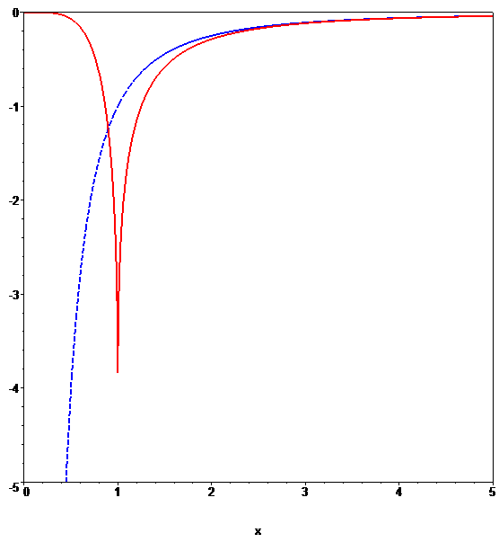
Second, the regulated potential vanishes at the origin but is greater in absolute value than the unregulated potential for . However, the difference is significant only for the lowest few , and the two potentials quickly converge as , as shown in Figure 1. The regulated and unregulated potentials hence differ significantly only near the singularity.
3.3 Eigenstates and the numerical method
We are now ready to look for the eigenstates of the Hamiltonian. Writing the eigenstate as and denoting the eigenvalue by , the regulated eigenvalue equation and the unregulated eigenvalue equation both give a recursion relation that takes the form
| (3.29) |
where (3.24) for the regulated potential and (3.19) for the unregulated potential. Note that the polymerization scale enters this recursion relation only in the combination , whether or not the potential is regulated. This is a direct consequence of the scale invariance of the potential.
From now on, we take and .
We use the “shooting method” that was applied in [12] to the polymerized potential. For large , (3.29) is approximated by
| (3.30) |
The linearly independent solutions to (3.30) are
| (3.31) |
The upper (respectively lower) sign gives coefficients that increase (decrease) exponentially as . We can therefore use (3.31) with the lower sign to set the initial conditions at large positive [31].
To set up the shooting problem, we choose a value for and begin with some to find and using the approximation (3.31). We then iterate downwards with (3.29). In the antisymmetric sector, we stop the iteration at and shoot for values of for which . This shooting problem is well defined both for the unregulated potential (3.18) and for the regulated potential (3.23), since the computation of via (3.29) does not require evaluation of at . In the symmetric sector, we stop at the iteration at and shoot for values of for which . As the computation of requires evaluation of at , the symmetric sector is well defined only for the regulated potential.
4 Results
We shall now compare the spectra of full polymer quantization, Bohr-Sommerfeld polymer quantization and ordinary Schrödinger quantization. We are particularly interested in the sensitivity of the results to the choice of the symmetric versus the antisymmetric sector.
First of all, we find that when the potential is regulated, the choice of the symmetric versus antisymmetric boundary condition in the full polymer quantum theory has no significant qualitative effect for sufficiently large , the only difference being slightly lower eigenvalues for the symmetric boundary condition. The lowest five eigenvalues in the two sectors are shown in Table 1 for . This is in a sharp contrast with what was found in [12] for the potential, where the symmetric sector contained a low-lying eigenvalue that appeared to tend to as the polymerization scale was decreased.
| antisymmetric | symmetric | |
|---|---|---|
| -6.14 | -6.37 | |
Another key feature is that for sufficiently large there is indeed a negative energy ground state. For , the plots of the lowest eigenvalues as a function of in Figures 2 and 3 show that the analytic lower bound obtained in subsection 3.2 is accurate within a factor of for the regulated potential in the antisymmetric sector and within a factor of two for the unregulated potential.
Figures 2 and 3 also indicate that the lowest eigenvalues converge towards zero as decreases, for both the unregulated and regulated potentials, with the unregulated eigenvalues reaching zero slightly before the regulated. Near the relationship is quadratic in while the plots straighten out to a linear relationship for larger .
The numerics become slow as the energies are close to zero. We were unable to investigate systematically whether bound states exist for , and in particular to make a comparison with the single bound state that occurs in Schrödinger quantization with certain self-adjoint extensions. For slightly below , we do find one bound state, but we do not know whether the absence of further bound states is a genuine property of the system of an artefact of insufficient computational power. This would be worthy of further investigation. The eigenvalues show a similar dependence on for both regulated and unregulated potentials, with the energies for the regulated potential being lower than those for the unregulated version as one would expect from comparing the potentials as in Figure 1.
For , we find that the eigenvalues depend on exponentially, except for the lowest few eigenvalues (). The coefficient in the exponent is in close agreement with the exact Schrödinger spectrum (2.11) and with the Bohr-Sommerfeld polymer spectrum (3.15) with . Representative spectra are shown as semi-log plots in Figures 4 and 5, where the linear fit is computed using only the points with . By matching the linear fit to the Schrödinger spectrum (2.11) and reading off the self-adjointness parameter , we can determine the self-adjoint extension of the Schrödinger Hamiltonian that matches the polymer theory for the highly-excited states. The results, shown in Figures 6 and 7, show that the self-adjointness parameter depends linearly on the coupling parameter , and the slope in this relation is within 10 per cent of the slope obtained from the Bohr-Sommerfeld estimate (3.16), (for , ).
Finally, our numerical eigenvalues are in excellent agreement with the analytic approximation scheme of [16], provided this scheme is understood as the limit of large with fixed . If the numerical results shown in figures 6 and 7 are indicative of the complementary limit of large with fixed , they show that the approximation scheme of [16] does not extend to this limit.
5 Conclusions
We have compared Schrödinger and polymer quantizations of the potential on the positive real line. The broad conclusion is that these quantization schemes are in excellent agreement for the highly-excited states and differ significantly only for the low-lying states. In particular, the polymer spectrum is bounded below, whereas the Schrödinger spectrum is known to be unbounded below when the coefficient of the potential term is sufficiently negative. We also find that the Bohr-Sommerfeld semiclassical quantization condition reproduces correctly the distribution of the highly-excited polymer eigenvalues. At some level this agreement is not surprising, since one expects that for any mathematically consistent quantization scheme, in some appropriate large , semi-classical limit, the spectra should agree. For anti-symmetric boundary conditions both Schrödinger and regulated and unregulated polymer obey the criteria, so it is perhaps not surprising that they agree at least for energies close to zero. It is somewhat surprising that they agree so well for low (where ”low” is in the context of the polymer spectra which are bounded below).
A central conceptual point was the regularization of the classical singularity in the polymer theory. We did this first by explicitly regulating the potential, using a finite differencing scheme that mimics the Thiemann trick used with the inverse triad operators in LQG [7]: this method allows a choice of either symmetric or antisymmetric boundary conditions at the origin. We then observed, as prevously noted in [16], that the singularity can alternatively be handled by leaving the potential unchanged but just imposing the antisymmetric boundary condition at the origin. The numerics showed that all of these three options gave very similar spectra, and the agreement was excellent for the highly-excited states.
To what extent is the agreement of these three regularization options specific to the potential? Consider the polymer quantization of the Coulomb potential, . When the Coulomb potential is explicitly regulated, it was shown in [12] that the choice between the symmetric and antisymmetric boundary conditions makes a significant difference for the ground state energy. We have now computed numerically the lowest five eigenenergies for the unregulated potential with the antisymmetric boundary condition, with the results shown in Table 2. Comparison with the results in [12] shows that the regularization of the potential makes no significant difference with the antisymmetric boundary condition. As noted in [12], for sufficiently small lattice spacing the antisymmetric boundary condition spectrum tends to that which is obtained in Schrödinger quantization with the conventional hydrogen s-wave boundary condition [10].
| 0 | -0.250 |
|---|---|
| 1 | -0.0625 |
| 2 | -0.0278 |
| 3 | -0.157 |
| 4 | -0.0100 |
We conclude that in polymer quantization of certain singular potentials, a suitably-chosen boundary condition suffices to produce a well-defined and arguably physically acceptable quantum theory, without the need to explicitly modify the classical potential near its singularity: the antisymmetric boundary condition effectively removes the eigenstate from the domain of the operator by requiring in the basis state expansion . A similar observation has been made previously in polymer quantization of a class of cosmological models, as a way to obtain singularity avoidance without recourse to the Thiemann trick [32, 33], and related discussion of the self-adjointness of polymer Hamiltonians arising in the cosmological context has been given in [34]. While we are not aware of a way to relate our system, with the potential and no Hamiltonian constraints, directly to a specific cosmological model, it is nonetheless reassuring that the various techniques we have used in this case for dealing with the singularity all lead to quantitatively similar spectra. Whether this continues to hold in polymer quantization of theories that are more closely related to LQG is an important open question that is currently under investigation [35].
Acknowledgements
We thank Jack Gegenberg, Sven Gnutzmann and Viqar Husain for helpful discussions and correspondence. GK and JZ were supported in part by the Natural Sciences and Engineering Research Council of Canada. JL was supported in part by STFC (UK) grant PP/D507358/1.
References
- [1] T. Thiemann, Modern Canonical Quantum General Relativity (Cambridge University Press, Cambridge, 2007).
- [2] A. Ashtekar, T. Pawlowski and P. Singh, “Quantum nature of the big bang: Improved dynamics,” Phys. Rev. D 74, 084003 (2006) [arXiv:gr-qc/0607039]; A. Ashtekar, T. Pawlowski, P. Singh and K. Vandersloot, “Loop quantum cosmology of k = 1 FRW models,” Phys. Rev. D 75, 024035 (2007) [arXiv:gr-qc/0612104]; K. Vandersloot, “Loop quantum cosmology and the RW model,” Phys. Rev. D 75, 023523 (2007) [arXiv:gr-qc/0612070]; M. V. Battisti, O. M. Lecian and G. Montani, “Polymer quantum dynamics of the Taub universe,” Phys. Rev. D 78, 103514 (2008) [arXiv:0806.0768 [gr-qc]].
- [3] M. Martin-Benito, L. J. Garay and G. A. Mena Marugan, “Hybrid Quantum Gowdy Cosmology: Combining Loop and Fock Quantizations,” Phys. Rev. D 78, 083516 (2008) [arXiv:0804.1098 [gr-qc]].
- [4] V. Husain and O. Winkler, “Quantum Hamiltonian for gravitational collapse,” Phys. Rev. D 73, 124007 (2006) [arXiv:gr-qc/0601082].
- [5] A. Ashtekar and M. Bojowald, “Quantum geometry and the Schwarzschild singularity,” Class. Quant. Grav. 23, 391 (2006) [arXiv:gr-qc/0509075].
- [6] L. Modesto, “Loop quantum black hole,” Class. Quant. Grav. 23, 5587 (2006) [arXiv:gr-qc/0509078]; “Black hole interior from loop quantum gravity,” arXiv:gr-qc/0611043; C. G. Boehmer and K. Vandersloot, “Loop Quantum Dynamics of the Schwarzschild Interior,” Phys. Rev. D 76, 104030 (2007) [arXiv:0709.2129 [gr-qc]]; “Stability of the Schwarzschild Interior in Loop Quantum Gravity,” Phys. Rev. D 78, 067501 (2008) [arXiv:0807.3042 [gr-qc]]; M. Campiglia, R. Gambini and J. Pullin, “Loop quantization of spherically symmetric midi-superspaces: the interior problem,” AIP Conf. Proc. 977, 52 (2008) [arXiv:0712.0817 [gr-qc]]; R. Gambini and J. Pullin, “Black holes in loop quantum gravity: the complete space-time,” Phys. Rev. Lett. 101, 161301 (2008) [arXiv:0805.1187 [gr-qc]].
- [7] T. Thiemann, “Quantum spin dynamics (QSD),” Class. Quant. Grav. 15, 839 (1998) [arXiv:gr-qc/9606089].
- [8] A. Ashtekar, S. Fairhurst and J. L. Willis, “Quantum gravity, shadow states, and quantum mechanics,” Class. Quant. Grav. 20, 1031 (2003) [arXiv:gr-qc/0207106].
- [9] H. Halvorson, “Complementarity of representations in quantum mechanics,” Studies Hist. Philos. Mod. Phys. 35, 45 (2004) [arXiv:quant-ph/0110102].
- [10] C. J. Fewster, “On the energy levels of the hydrogen atom,” arXiv:hep-th/9305102.
- [11] J. Louko and J. Mäkelä, “Area spectrum of the Schwarzschild black hole,” Phys. Rev. D 54, 4982 (1996) [arXiv:gr-qc/9605058].
- [12] V. Husain, J. Louko and O. Winkler, “Quantum gravity and the Coulomb potential,” Phys. Rev. D 76, 084002 (2007) [arXiv:0707.0273 [gr-qc]].
- [13] L. Motl, “An analytical computation of asymptotic Schwarzschild quasinormal frequencies,” Adv. Theor. Math. Phys. 6, 1135 (2003) [arXiv:gr-qc/0212096].
- [14] G. Kunstatter, “d-dimensional black hole entropy spectrum from quasi-normal modes,” Phys. Rev. Lett. 90, 161301 (2003) [arXiv:gr-qc/0212014].
- [15] H. E. Camblong and C. R. Ordonez, “Black hole thermodynamics from near-horizon conformal quantum mechanics,” Phys. Rev. D 71, 104029 (2005) [arXiv:hep-th/0411008].
- [16] J. Gegenberg, G. Kunstatter and R. D. Small, “Quantum structure of space near a black hole horizon,” Class. Quant. Grav. 23, 6087 (2006) [arXiv:gr-qc/0606002].
- [17] K. M. Case, “Singular Potentials,” Phys. Rev. 80, 797 (1950).
- [18] W. M. Frank, D. J. Land and R. M. Spector, “Singular Potentials,” Rev. Mod. Phys. 43, 36 (1971).
- [19] H. Narnhofer, “Quantum theory for -potentials,” Acta Phys. Austriaca 40, 306 (1974).
- [20] K. S. Gupta and S. G. Rajeev, “Renormalization in quantum mechanics,” Phys. Rev. D 48, 5940 (1993) [arXiv:hep-th/9305052].
- [21] H. E. Camblong, L. N. Epele, H. Fanchiotti and C. A. Garcia Canal, “Renormalization of the inverse square potential,” Phys. Rev. Lett. 85, 1590 (2000) [arXiv:hep-th/0003014]; “Dimensional transmutation and dimensional regularization in quantum mechanics. I: General theory,” Annals Phys. 287, 14 (2001) [arXiv:hep-th/0003255].
- [22] H. E. Camblong and C. R. Ordonez, “Renormalization in conformal quantum mechanics,” Phys. Lett. A 345, 22 (2005) [arXiv:hep-th/0305035]; “Anomaly in conformal quantum mechanics: From molecular physics to black holes,” Phys. Rev. D 68, 125013 (2003) [arXiv:hep-th/0303166]; G. N. J. Ananos, H. E. Camblong and C. R. Ordonez, “SO(2,1) conformal anomaly: Beyond contact interactions,” Phys. Rev. D 68, 025006 (2003) [arXiv:hep-th/0302197].
- [23] H. E. Camblong, L. N. Epele, H. Fanchiotti, C. A. Garcia Canal and C. R. Ordonez, “On the Inequivalence of Renormalization and Self-Adjoint Extensions for Quantum Singular Interactions,” Phys. Lett. A 364, 458 (2007) [arXiv:hep-th/0604018].
- [24]
T. Fúlöp, Symmetry, Integrability and Geometry, Proceedings of the 3rd Microconference “Analytic and Algebraic Methods III”, http://www.emis.de/journals/SIGMA/Prague2007.html
- [25] W. E. Thirring, Quantum mathematical physics, 2nd edition (Springer, Berlin, 2002).
- [26] Handbook of Mathematical Functions, edited by M. Abramowitz and I. A. Stegun (Dover, New York, 1965).
- [27] A. Corichi, T. Vukasinac and J. A. Zapata, “Polymer Quantum Mechanics and its Continuum Limit,” Phys. Rev. D 76, 044016 (2007) [arXiv:0704.0007 [gr-qc]].
- [28] N. Andersson and C. J. Howls, “The asymptotic quasinormal mode spectrum of non-rotating black holes,” Class. Quant. Grav. 21, 1623 (2004) [arXiv:gr-qc/0307020].
- [29] I. S. Gradshteyn and I. M. Ryzhik, Table of Integrals, Series and Products, 4th edition (Academic, New York, 1980).
- [30] M. Reed and B. Simon, Methods of Modern Mathematical Physics II: Fourier Analysis, Self-adjointness (Academic, New York, 1975).
- [31] S. Elaydi, An Introduction to Difference Equations, 3rd edition (Springer, New York, 2005).
- [32] A. Ashtekar, A. Corichi and P. Singh, “On the robustness of key features of loop quantum cosmology,” Phys. Rev. D 77, 024046 (2008) [arXiv:0710.3565 [gr-qc]].
- [33] A. Corichi and P. Singh, “Is loop quantization in cosmology unique?,” Phys. Rev. D 78, 024034 (2008) [arXiv:0805.0136 [gr-qc]].
- [34] W. Kaminski and J. Lewandowski, “The flat FRW model in LQC: the self-adjointness,” Class. Quant. Grav. 25, 035001 (2008) [arXiv:0709.3120 [gr-qc]].
- [35] G. Kunstatter, J. Louko and J. Ziprick, in progress.