In an attempt to implement gauge mediation in string theory, we study string effective supergravity models of supersymmetry breaking, containing anomalous gauge factors. We discuss subtleties related to gauge invariance and the stabilization of the Green-Schwarz moduli, which set non-trivial constraints on the transmission of supersymmetry breaking to MSSM via gauge interactions. Given those constraints, it is difficult to obtain the dominance of gauge mediation over gravity mediation. Furthermore, generically the gauge contributions to soft terms contain additional non-standard terms coming from D-term contributions. Motivated by this, we study the phenomenology of recently proposed hybrid models, where gravity and gauge mediations compete at the GUT scale, and show that such a scenario can respect WMAP constraints and would be easily testable at LHC.

1 Introduction

Recently there was some renewed interest in implementing gauge mediation [1] in explicit supergravity framework and in string theory [2, 3, 4, 5, 6, 7]. In models without anomalous $U(1)$ symmetries, gauge mediation contribution to the soft supersymmetry breaking terms naturally dominates over gravity mediation contributions [8, 9]. This happens, for example, adding messengers in models of F-term uplift [9]. However, it is difficult to to find string origin of such models. In string constructions, there are generically present anomalous $U(1)$ symmetries and the messenger fields, which are typically bifundamentals between SM gauge factors and the $U(1)$ ’s, are charged under them, as well as the Green-Schwarz moduli responsible for anomaly cancellation. It is therefore important to study if the dominance of gauge mediation can be obtained in models where $U(1)$ symmetry plays important role in the supersymmetry breaking sector. Several explicit string models attempting to implement gauge mediation in the presence of anomalous $U(1)$ have been recently constructed [2, 3, 4, 5, 6, 7] and it is generally believed that this framework can naturally provide a viable gauge mediation transmission of supersymmetry breaking. However, as pointed out recently in a particular example [4], there are some subtleties to take into account if D-term contributions are present in this case.

The purpose of the present paper is to enter more into the structure of these class of models and the various constraints arising from:

i)

gauge invariance via the Green-Schwarz mechanism;
ii)

stabilization of the Green-Schwarz moduli fields;
iii)

avoiding a Fayet-Iliopoulos term for the hypercharge and the existence of non-standard gauge contributions to the MSSM soft terms, which naturally arise in the presence of D-terms for $U(1)$ ’s under which messengers are charged, with important phenomenological consequences;

We show that the correct implementation of these constraints implies that it is hard to parametrically strongly suppress gravity contributions compared to the gauge ones, though some dominance of gauge mediation, easing the FCNC problems of gravity, is possible in some regions of the parameter space. Compared to uplifting models without $U(1)$ ’s, the difference is that gauge invariance strongly correlates supersymmetry breaking to the sector of moduli stabilization through the gauge scalar potential. This translates into the fact that the moduli-dependent Fayet-Iliopoulos term cannot be parametrically much smaller than the Planck mass. Thus, the vev of the field $S$ breaking SUSY is large¹¹ 1 Most of the expressions are presented in Planck units, namely, we set $M_{P}=1$ . However, at some instances, we keep $M_{P}$ explicitly to make the discussions clearer. $10^{-1}\leq S\leq 10^{-3}$ and as a result there is a phenomenological lower limit on the gravitino mass $m_{3/2}\raise 1.29167pt\hbox{$\;>$\kern-7.5pt\raise-4.73611pt\hbox{$\sim\;$}}50-100$ GeV . In addition, there are additional non-standard gauge mediation contributions. For example, constraint iii) is hard to satisfy in some models with non-zero D-terms [3, 5], whereas in models with zero D-terms [7] implementation of i) and ii) generically creates new supersymmetric vacua.

In fact, once the above constraints are carefully taken into account, one is led to a class of “hybrid” models, where both gravity mediation and gauge mediation are equally important. In the second part of this paper we therefore pursue in some detail a generalization of the model introduced in [4] where the above constraints are taken into account.

High energy physics approaches a new era with the LHC. It will be possible to test a much larger part of the parameter space of SUSY models, exclude some of them, or confirm the presence of supersymmetric particles. Through the measurement of physical parameters (masses, couplings, branching ratios), we will be able to extract fundamental informations on the SUSY breaking mechanism: gauge, gravity, anomalous $U(1)$ mediation [10], the anomaly mediation [11], gaugino mediation [12], mirage mediation [13], etc.

Here we point out that in the presence of anomalous $U(1)$ and messenger fields, charged under $U(1)$ and under the SM gauge groups, one naturally obtains another type of mixed supersymmetry breaking transmission mechanism, gravity and gauge mediation, with interesting phenomenological signatures.

2 Gauge models of supersymmetry breaking and moduli stabilization

Both main mechanisms of supersymmetry breaking, Fayet-Iliopoulos (FI) [14] and O’Raifeartaigh (O’R) [15] contain mass scales, which fix the scale of supersymmetry breaking. If the mediation of supersymmetry breaking is by Standard Model gauge interactions, the corresponding mass scales are typically low. In the case of the gravity mediation, they are typically at intermediate energy scales. In both cases, a dynamical origin for these values, small in Planck units, is needed. The traditional viewpoint was to invoke some field theoretical nonperturbative effects in a sector which dynamically breaks supersymmetry. With the more recently studied stringy instantonic effects [17], there is the possibility of replacing field-theoretical nonperturbative effects with stringy instanton effects which are computable in string theory. These effects give mass scales of order

m_{i}\sim e^{S_{\rm inst}}\quad,\quad{\rm where}\quad S_{inst}=\sum_{m}c_{m}T_{m}

(1)

is an instantonic action depending on moduli fields related to the cycle(s) the instantonic brane is wrapping. In all effective string models we are aware, there are abelian gauge factors which are gauged by some of the moduli fields, generating a Green-Schwarz mechanism of anomaly cancelations. The crucial point we would like to insist in what follows is that, while finding string effective models reproducing at low-energy the basic features of the FI or the O’R model in this framework is relatively easy, the dynamics of the moduli fields $T_{m}$ set severe constraints on the transmission of supersymmetry breaking.

Let us start with a quick reminder of some basic results in ${\cal N}=1$ supergravity with $U(1)$ gauged symmetries. As a starting point, let us recall that the scalar potential in supergravity has the following form:

V=e^{G}(G^{M}~G_{M}-3)+{1\over 2}\sum_{A}g_{A}^{2}D_{A}^{2}\ ,

(2)

where

G\ =\ {\cal K}\ +\ \log|W|^{2}\ ,

(3)

and $G_{M}={\partial G\over\partial z^{M}},$ where $z$ represents the scalar part of a chiral superfield. The index $M$ runs over all the chiral superfields present, matter as well as hidden sector and/or moduli fields. On the other hand, the auxiliary D-terms are given by

D_{A}=z^{I}T_{IJ}^{A}{\partial G\over\partial z^{J}}~+~\xi_{A}={\bar{z}}^{\bar{I}}T_{IJ}^{A}{\partial G\over\partial{\bar{z}}^{\bar{J}}}~+~\xi_{A}\ ,

(4)

where $T^{A}$ represents the generators of the gauge group with index $A$ and $\xi_{A}$ denotes the Fayet-Iliopoulos terms for the abelian $U(1)$ factors. Note that the equality between the two last terms is a straightforward consequence of the gauge invariance of the Kähler potential. We take into account the fact that in string theory, the Fayet-Iliopoulos terms are moduli-dependent.

In the presence of anomalous non-linearly realized abelian gauge symmetries

	$\displaystyle\delta V_{A}\ =\ \Lambda_{A}+{\bar{\Lambda}}_{A}\quad,\quad\delta z^{i}\ =\ 2X_{i}^{a}\ z^{i}\ \Lambda_{A}\ ,$
	$\displaystyle\delta T^{\alpha}\ =\ \delta_{A}^{\alpha}\ \Lambda_{A}\ ,$		(5)

the auxiliary D-terms are defined as

D_{A}\ =\ z^{i}\ X_{i}^{A}\ \partial_{i}G\ -\ {\delta_{A}^{\alpha}\over 2}\ \partial_{\alpha}G\ .

(6)

The last term in (6) is the moduli-dependent FI term

\xi_{A}\ =\ -\ {\delta_{A}^{\alpha}\over 2}\ \partial_{\alpha}G\ .

(7)

In the following we will often use the standard definition of F-terms

F^{i}\ =\ e^{{\cal K}\over 2}\ {\cal K}^{i{\bar{j}}}\ \overline{D_{j}W}\ ,

(8)

where $D_{j}W=\partial_{j}W+W\partial_{j}K$ , such that (6) becomes

m_{3/2}\ D_{A}\ =\ z^{i}\ X_{i}^{A}\ F_{i}\ -\ {\delta_{A}^{\alpha}\over 2}\ F_{\alpha}\ ,

(9)

where as usual $m_{3/2}=\exp({\cal K}/2)W$ . Eq. (9) tells us that the supersymmetric $D$ and the $F$ conditions are not independent. Therefore in order to find supersymmetric solutions it is enough to check the minimum independent number of SUSY conditions.

Some comments are in order concerning moduli masses. In models with anomalous $U(1)$ and FI term much larger than the gravitino mass, which is the case of interest in string theory and is the case considered throughout this paper, there is always a charged field, of appropriate charge and large vev that compensates to a good accuracy the FI term. This field is always heavier than the Kähler modulus transforming non-linearly under $U(1)$ , which has masses of the order (or slightly larger) than the gravitino mass. In the case of a twisted modulus, its mass is generically of the order of the string scale and therefore generically very heavy. Even in this case which suggests that the twisted modulus is irrelevant at low energy and therefore can integrated out, this has to be done with care. Indeed, as we will see in detail later on, supergravity approximation and gauge domination would require a very small vev for the twisted modulus. The explicit dynamics of the modulus, on the other hand, constrained by gauge invariance, often prefers large vev’s.

2.1 Dominance of gauge mediation over gravity mediation

In a generic model with (almost) Minkowski vacuum, and with $F$ -terms larger than the $D$ -terms, the uplifting condition requires a cancelation between the $F$ -term contribution to the vacuum energy and the SUGRA correction $-3m_{3/2}^{2}$ . This implies that in a viable SUSY breaking minimum no $F$ -term can be much larger than $m_{3/2}$ . On the other hand, if SUSY is broken by some field S, coupled to the messengers²² 2 We take $S$ to have standard Kähler potential for simplicity., then dominance of gauge mediation over gravity mediation requires

\frac{g^{2}}{16\pi^{2}}\frac{\langle F_{S}\rangle}{\langle S\rangle}\ \gg\ m_{3/2}\ .

(10)

Thus, we have gauge mediation dominance only if $\langle S\rangle\ll 1$ , i.e. if the messenger masses $m\sim\langle S\rangle$ are very small in Planck units. Since $F_{S}\sim\sqrt{3}m_{3/2}M_{P}$ , we can define the ratio between the gauge and gravity contributions to soft terms as

{M_{GM}\over m_{3/2}}\ \equiv\ g^{2}\ \alpha\ \equiv{g^{2}\over 8\pi^{2}}\ \sqrt{3}\ N\ {M_{P}\over S}\ ,

(11)

where $N$ is the number of messengers and $g$ a Standard Model gauge coupling. In a (minimal) model with only one field $S$ charged under some anomalous $U(1)_{X}$ , the value of $S$ is roughly set by the value of the FI terms $\xi$ , so that we can have a small $\langle S\rangle$ only in the presence of a small $\xi$ . By fixing $\xi$ to be very small, we are always enhancing the contribution of gauge mediation over the gravity mediation.

On the other hand, as explained above in (7), $\xi$ is moduli-dependent and its value is fixed by the dynamics. We cannot assume that $\xi$ is fixed by some independent dynamics “at high scale”, since such a dynamics involves moduli stabilization, that affects the form of the $D$ -term potential. The problems stated here could perhaps be avoided but only in a complicated generalization of the minimal constructions, including more than one modulus field.

In what follows we show in detail how the minimal setups fail in achieving gauge mediation dominance, due to the large vev’s of $S\raise 1.29167pt\hbox{$\;>$\kern-7.5pt\raise-4.73611pt\hbox{$\sim\;$}}10^{-3}$ and show a model where only a marginal dominance $\alpha\raise 1.29167pt\hbox{$\;<$\kern-7.5pt\raise-4.73611pt\hbox{$\sim\;$}}100$ is allowed for a large number of messengers. Then, as discussed later, experimental constraints on superpartner masses imply that there is lower limit on the gravitino mass $m_{3/2}\raise 1.29167pt\hbox{$\;>$\kern-7.5pt\raise-4.73611pt\hbox{$\sim\;$}}50-100$ GeV. The resulting, hybrid phenomenology, will be the main subject of section 5.

2.2 Gauged Polony model and SUSY vacua

The simplest model falling in the description given above contains one single field $S$ with a linear superpotential term $W\supset\lambda S$ breaking SUSY. In order to have a viable model, $\lambda$ should be small, thus sourced by some instantonic effects involving, in a minimal string setup, one modulus field $T$ : $\lambda\sim e^{-\alpha T}$ . Assuming $S$ to be charged under a $U(1)_{X}$ , as it is always the case in a string model, gauge invariance forces $T$ to have an anomalous variation. Thus, under the gauge transformation $V\rightarrow V+\Lambda+\bar{\Lambda}$ , we have $S\rightarrow Se^{-2q_{S}\Lambda}$ and $T\rightarrow T+\delta_{GS}\Lambda$ , $q_{S}$ being the $S$ $U(1)_{X}$ charge. We use the notation $\delta_{GS}$ since we expect the anomalous $T$ variation³³ 3 If we force $T=T_{0}$ this is the model recently studied in [7] to be linked with an anomaly cancellation in a string models, via the Green-Schwarz mechanism, i.e. we expect $T$ to be part of some gauge kinetic function. Taking $q_{S}=-1$ we have

	$\displaystyle W\ =\ W_{0}\ +\ ae^{-{2T\over\delta_{GS}}}\ S\ ,\$
	$\displaystyle{\cal K}\ =\ S^{\dagger}e^{-2V}S\ +\ K(T+{\bar{T}}-\delta_{GS}V)\ ,$
	$\displaystyle D\ =\ -\|S\|^{2}\ -\ {\delta_{GS}\over 2}\ \partial_{T}K\ ,$		(12)

where the last term in the $D$ -term is the field dependent FI term due to the anomalous $T$ variation. In this model, the relation (9) between $F$ -terms and $D$ -terms can be rewritten as

\displaystyle S\ F_{S}\ +\ \frac{\delta_{GS}}{2}\ F_{T}\ =\ -\ D\ m_{3/2}

(13)

and a SUSY minimum is ensured if

D=-|S|^{2}-\frac{\delta_{GS}}{2}\partial_{T}K=0,\quad e^{-{\cal K}/2}F_{S}=ae^{-\frac{2T}{\delta_{GS}}}+\bar{S}W=0\ .

(14)

These two equations generically have solution, but the specific details depend on the form of $K(T+{\bar{T}}-\delta_{GS}V)$ . In what follows we consider some cases of particular relevance in a string theory setup: first we study the case in which $T$ is a standard Kähler modulus, with logarithmic potential, then we consider the case of a twisted modulus, with polynomial potential. Finally we consider the generalization to the case in which the sector of moduli contains more than one modulus field.

Our aim is to show that under very general assumptions, it is difficult to have dominance of gauge mediation over gravity mediation, since no viable minimum is present with $\langle S\rangle\ll 1$ .

T as a standard Kähler modulus

In this case

K=-3\,\log(T+{\bar{T}}-\delta_{GS}V)\ ,

(15)

thus the SUSY conditions can be rewritten, neglecting the imaginary parts of $S$ and $T$ , as

\displaystyle D=-|S|^{2}+\frac{3\delta_{GS}}{2(T+\bar{T})}=0,\quad e^{-{\cal K}/2}F_{S}=ae^{-\frac{3}{2|S|^{2}}}(1+|S|^{2})+\bar{S}W_{0}=0\ .

(16)

The first equation fixes $T$ as a function of $S$ , then $T$ was substituted in the condition $F_{S}=0$ . The second equation has a solution for $|S|^{2}\rightarrow 0$ , corresponding to the runaway $T\rightarrow\infty$ . In the case $W_{0}\ll a$ there is another SUSY solution for $\langle S\rangle\ll 1$ , and $T\gg 1$ . Since typically $a\sim{\cal O}(1)$ , we have that in such a model, for essentially all the reasonable values of $W_{0}$ , there is a SUSY minimum in a viable region for $\langle S\rangle$ and $\langle T\rangle$ and therefore this model does not break SUSY.

Moreover, even in case a metastable SUSY breaking vacuum is found, we can infer, on a very general basis, that it is impossible to obtain a pure gauge mediation scenario. After coupling $S$ to some messenger fields, we immediately find that the condition $\langle S\rangle\ll 1$ is incompatible with the original supergravity dynamics. In fact, from $D$ -flatness one finds that the instantonic effect is of order

e^{-{2T\over\delta_{GS}}}\ =\ e^{-{3\over 2S^{2}}}\ .

(17)

In other words, the requirement of a very small FI term kills the SUSY breaking effects.

T as a twisted Kähler modulus

In this case we expect $T\ll 1$ , thus, the non-perturbative effects are suppressed only assuming the gauge kinetic function to depend on some extra modulus $M$ , having no transformation under the anomalous $U(1)_{X}$ . Since $M$ is invariant under a $U(1)_{X}$ transformation, it does not enter in the $D$ -term, its dynamics is not constrained by gauge invariance, and it is reasonable to assume some hidden dynamics to stabilize it at high scale and large vev. In this way, the net effect of $M$ is a small prefactor $a$ in front of the instantonic superpotential term. Given the Kähler potential

K=\frac{1}{2}(T+{\bar{T}}-\delta_{GS}V)^{2}\ +\ S^{\dagger}e^{-2V}S\ ,

(18)

the SUSY conditions can be rewritten as

\displaystyle D=-|S|^{2}-\frac{\delta_{GS}}{2}(T+\bar{T})=0,\quad e^{-{\cal K}/2}F_{S}=ae^{\frac{2|S|^{2}}{\delta_{GS}^{2}}}(1+|S|^{2})+\bar{S}W_{0}=0,

(19)

where we assume $\delta_{GS}<0$ , and we neglected the imaginary parts of $T$ and $S$ . Thus, under the assumption $S\ll 1$ we find viable SUSY solutions only for $a\ll W_{0}$ : $S\sim-a/W_{0}$ . In other words, in case $a\ll W_{0}$ a SUSY solution is present at $S\sim-a/W_{0}$ . Moreover, in the limit $a\ll W_{0}$ it’s easy to check that any non-SUSY minimum eventually present, with $S\ll 1$ , cannot be uplifted, since $F_{S},\,F_{T}\ll m_{3/2}$ . Thus, the only viable regime of the parameters is $a\gg W_{0}$ , but in such a case the requirement $S\ll 1$ forces $F_{S}\gg m_{3/2}$ . This implies that no cancelation between $F_{S}$ and $W$ is possible, so that the cosmological constant is set by the $F_{S}$ value to be larger than the gravitino mass. Of course, one could in principle hope a viable SUSY breaking minimum to be present in case $a\sim W_{0}$ , where the problems raised above could be absent. On the other hand, it is unreasonable to expect such a minimum for small values of $\langle S\rangle$ . Indeed, assuming $a\ll 1$ we see that the $D$ -term contribution will fix $S$ close to the modulus vev (or vice-versa), plus $O(a)$ corrections. Replacing this in the other equation we essentially get just an algebraic function with order one parameters, multiplied by an overall energy scale $a^{2}$ . Thus, no extrema exist at small $S$ (as it can also be checked by direct inspection).

Extensions to a generic number of moduli fields

A natural extension is to consider more than one modulus to be charged under the anomalous $U(1)_{X}$ . Let us consider $n$ moduli $T_{i}$ , $i=1,\dots n$ with Kähler potential⁴⁴ 4 In the case in which the moduli are all “twisted” we get results similar to the single twisted modulus case.

K\ =\ -\ \sum_{i}p_{i}\,\log(T_{i}+\bar{T}_{i}-\delta_{i}V)\ ,

(20)

the superpotential

W\ =\ W_{0}\ +\ ae^{-\sum_{i}b_{i}T_{i}}S

(21)

with $\sum b_{i}\delta_{i}=2$ and the D-term

D=-|S|^{2}+\sum_{i}\frac{p_{i}\delta_{i}}{2}\frac{1}{T_{i}+\bar{T}_{i}}\ ,

(22)

while the $F$ -terms are

	$\displaystyle e^{-{\cal K}/2}F_{S}=\bar{S}W+ae^{-\sum_{i}b_{i}T_{i}}\ ,$
	$\displaystyle e^{-{\cal K}/2}F_{T_{i}}=-\frac{p_{i}}{T_{i}+\bar{T}_{i}}W\ -\ ab_{i}\ e^{-\sum_{i}b_{i}T_{i}}S\ .$		(23)

A SUSY solution is present if we have all F-terms equal to zero. Thus, we can replace the condition $F_{S}=0$ in the other conditions and find

\displaystyle\frac{p_{i}}{T_{i}+\bar{T}_{i}}\ =\ b_{i}\ |S|^{2}\ .

(24)

These conditions, that also imply $D=0$ , fix the real parts of $T_{i}$ as functions of $S$ . Thus, neglecting the $T_{i}$ phases, we can replace them in the eq. $F_{S}=0$ to find

\bar{S}\ W\ +\ ae^{-\frac{\sum_{i}p_{i}}{2|S|^{2}}}=0\ ,

(25)

that is, de facto, the same condition found in the single (untwisted) modulus case, having solution in all the reasonable regimes for $W$ , and with the same (negative) implications for what concerns the issue of gauge mediation dominance.

A natural “complication” arising in the presence of more than one modulus is the presence of extra instantonic effects, so that

W\supset\sum_{j}e^{-\sum_{i}\alpha^{j}_{i}T_{i}},

(26)

with $\sum\alpha^{j}_{i}\delta_{i}=0$ for each $j$ , due to gauge invariance. Such new terms can have an important rôle in the stabilization of the moduli fields, but it is clear that the F-term equations will be generically solvable, and we expect a generic model to have a SUSY minimum in some viable parameters region. Of course, in very specific models the minima could be located at unacceptable values of the moduli fields, and extra SUSY breaking minima could be present. On the other hand, in such a case it would be precisely the moduli sector the main actor and the most interesting part of the whole SUSY breaking mechanism. In such a generalization one could hope to avoid the constraint of Eq. (25), and fix the moduli so to have a small induced FI term without destroying the instantonic effect breaking SUSY. Such a model would be a good candidate for a model realizing gauge mediation in a realistic string model.

2.3 Fayet-O’Raifeartaigh models

The simplest model in this class is again based on a $U(1)_{X}$ gauge symmetry with a O’R like superpotential

	$\displaystyle W\ =\ W_{0}\ +\phi_{--}(\lambda_{1}\phi_{+}^{2}-m^{2}e^{-{4T\over\delta_{GS}}})\ +\ \lambda_{2}\ \chi_{--}\phi_{+}^{2}\ ,\$
	$\displaystyle{\cal K}\ =\ \phi_{+}^{\dagger}e^{2V}\phi_{+}+\phi_{--}^{\dagger}e^{-4V}\phi_{--}+\chi_{--}^{\dagger}e^{-4V}\chi_{--}+K(T+{\bar{T}}-\delta_{GS}V)\ ,$
	$\displaystyle D\ =\ -2\ \|\phi_{--}\|^{2}\ -\ 2\ \|\chi_{--}\|^{2}+\|\phi_{+}\|^{2}-{\delta_{GS}\over 2}\ \partial_{T}K\ .$		(27)

It is easy to check that in the supersymmetry breaking vacuum, we have

	$\displaystyle{\bar{F}}_{\phi_{+}}=0\qquad\qquad{\bar{F}}_{\phi_{--}}=-\frac{\lambda_{2}}{\lambda_{1}}{\bar{F}}_{\chi_{--}}=-\frac{\lambda_{2}^{2}m_{0}^{2}}{\lambda_{1}^{2}+\lambda_{2}^{2}}\qquad\qquad D=0$		(28)
	$\displaystyle\|\phi_{+}\|^{2}=\left\|\frac{\lambda_{1}m_{0}^{2}}{\lambda_{1}^{2}+\lambda_{2}^{2}}\right\|\qquad\left\|\phi_{--}\right\|^{2}=\frac{\lambda_{2}^{2}}{\lambda_{1}^{2}}\left\|\chi_{--}\right\|^{2}=\frac{1}{2}\left(\xi_{FI}^{2}+\left\|\frac{\lambda_{1}m_{0}^{2}}{\lambda_{1}^{2}+\lambda_{2}^{2}}\right\|\right)\frac{\lambda_{2}}{\lambda_{1}^{2}+\lambda_{2}^{2}}$

where we have defined $\xi_{FI}^{2}=-{\delta_{GS}\over 2}\ \partial_{T}K$ and $m_{0}^{2}=\exp(K/2)m^{2}\exp(-4T/\delta_{GS})$ . About the chance of having gauge mediation dominance, we observe that

\left|\frac{F_{\phi_{--}}}{\phi_{--}}\right|^{2}=\left|\frac{F_{\chi_{--}}}{\chi_{--}}\right|^{2}=\frac{2\lambda_{2}^{2}m_{0}^{4}}{\left(\lambda_{1}^{2}+\lambda_{2}^{2}\right)}\frac{1}{\xi_{FI}^{2}+\left|\frac{\lambda_{1}m^{2}}{(\lambda_{1}^{2}+\lambda_{2}^{2})}\right|}<\frac{6m_{3/2}^{2}}{\xi_{FI}^{2}}\ .

(29)

Once again, the only possibility to have pure gauge mediation requires $\xi_{FI}^{2}\ll 1$ , but this is incompatible with moduli stabilization, at least in case we have a single modulus with logarithmic Kähler potential.

2.4 Fayet-Iliopoulos and Fayet-Polony models

The simplest generalization of the basic Fayet-Iliopoulos model is described by an $U(1)_{X}$ gauge symmetry and two charged fields $\phi_{\pm}$ , plus a mass term:

	$\displaystyle W\ =\ W_{0}\ +\ e^{-M}\phi_{+}\phi_{-}\ ,\$
	$\displaystyle{\cal K}\ =\ \phi_{+}^{\dagger}e^{2V}\phi_{+}+\phi_{-}^{\dagger}e^{-2V}\phi_{-}+K_{0}(M+{\bar{M}})+K(T+{\bar{T}}-\delta_{GS}V)\ ,$
	$\displaystyle D\ =\ \|\phi_{+}\|^{2}-\|\phi_{-}\|^{2}-{\delta_{GS}\over 2}\partial_{T}K\ ,$		(30)

where the last term is the field-dependent FI parameter. Under gauge transformations, the various fields transform as

	$\displaystyle V\rightarrow V+\Lambda+{\bar{\Lambda}}\quad,\quad\phi_{\pm}\rightarrow e^{\mp 2\Lambda}\phi_{\pm}\ ,$
	$\displaystyle T\rightarrow T+\delta_{GS}\ \Lambda\ .$		(31)

Since $T$ is (nonlinearly) charged under $U(1)_{X}$ whereas the operator $\phi_{+}\phi_{-}$ is neutral, the instantonic action generating the mass term $m\sim e^{-M}$ cannot depend on $T$ , but it should depend on another, $U(1)_{X}$ neutral modulus (or linear combination of moduli) $M$ . The constant $W_{0}$ in (30) was added for two reasons. First, it will help to adjust the cosmological constant to zero in a supergravity framework. Secondly, as well-known, it also plays an instrumental role in moduli stabilization. This model has the feature that, if the moduli fields are assumed to be stabilized, in the rigid (global) limit it reduces to the FI model of supersymmetry breaking. From the point of view of moduli stabilization, however, the model (30) is not very satisfactory, since there are two moduli fields, $M$ and $T$ to stabilize. Whereas $M$ could be stabilized by string theory fluxes, along the lines of [18] and simultaneously generating $W_{0}$ , $T$ cannot be stabilized without further dynamics.
A more viable model is what we could call a Fayet-Polony model, with the same Kähler potential and D-term as in (30), whereas the superpotential is

W\ =\ W_{0}\ +\ e^{-M}\phi_{+}\phi_{-}\ +\ e^{-2qT/\delta_{GS}}\phi_{-}^{q}\ .

(32)

The powers $q$ are selected such that $2qT/\delta_{GS}$ represents an integer of the instanton action. By assuming as above that $M$ is stabilized by fluxes (or that the mass $m=\exp(-M)$ is generated by field-theory nonperturbative dynamics), this model was analyzed in detail in [4] for the case of the volume-type $T$ modulus

K\ =\ -3\ \log(T+{\bar{T}}-\delta_{GS}V)\ .

(33)

Strictly speaking, only $q=1$ corresponds to a linear, Polony-like term, but since $\phi_{-}$ tends to compensate the FI term and to get a large vev, the dynamics of the model is not qualitatively different for $q=1$ and $q\not=1$ . It is conceptually transparent that in a model like (32) moduli stabilization cannot be ignored. First of all, the modulus mass $T$ has a mass that, for large FI term is parametrically smaller than the mass of $\phi_{-}$ so cannot be consistently integrated out. Secondly, even if this could be possible, freezing out $T$ in (32) gives a gauge non-invariant lagrangian. The computation of any physical quantity done in this way differs considerably from the computation done by keeping the modulus dynamics. In the following sections of the present paper we show that only a moderate dominance is possible in very specific regions of the parameter space.

2.4.1 SUSY minima in the Fayet-Polony model

We think the modulus $M$ stabilized at high energy ⁵⁵ 5 Note that this is possible only because the modulus $M$ can decouple from the dynamics of the $U(1)_{X}$ sector. and replace it with a constant $m=e^{-M}$ in the model (32). A complete analysis of the vacuum structure of this model has already been done in [4] and extended in the next sections. Here we explicitly show the role of the parameter $m$ in determining the presence or the absence of the supersymmetric solution. For example, the relation between F-terms and D-term in the case $q=1$ , reads

\phi_{+}F_{+}-\phi_{-}F_{-}-\frac{\delta_{GS}}{2}F_{T}\ =\ D~m_{3/2}\ .

(34)

It is then enough to search for solutions of the following equations

$\displaystyle e^{-{\cal K}/2}F_{+}$	$\displaystyle=$	$\displaystyle m\phi_{-}+{\bar{\phi}}_{+}W=0\ ,$
$\displaystyle e^{-{\cal K}/2}F_{-}$	$\displaystyle=$	$\displaystyle m\phi_{+}+ae^{-2T/\delta_{GS}}+{\bar{\phi}}_{-}W=0\ ,$
$\displaystyle D$	$\displaystyle=$	$\displaystyle\|\phi_{+}\|^{2}-\|\phi_{-}\|^{2}-\frac{\delta_{GS}}{2}\partial_{T}K=0\ .$	(35)

It is straightforward to see that the model has a possible SUSY vacuum for

$\displaystyle\phi_{+}$	$\displaystyle=$	$\displaystyle-\frac{{\bar{m}}}{{\bar{W}}}{\bar{\phi}}_{-}\ ,$
$\displaystyle\phi_{-}$	$\displaystyle=$	$\displaystyle\frac{ae^{-2{\bar{T}}/\delta_{GS}}~W}{\|m\|^{2}-\|W\|^{2}}\ ,$
$\displaystyle\partial_{T}K$	$\displaystyle=$	$\displaystyle\frac{2}{\delta_{GS}}\frac{\|ae^{-2{\bar{T}}/\delta_{GS}}\|^{2}}{\left(\|m\|^{2}-\|W\|^{2}\right)}\ .$	(36)

However, the last equation shows that, depending on the sign of $\partial_{T}K$ , a solution is allowed in different regions of the parameters space. In particular, focusing on the case of a standard Kähler modulus $T$ (33), the equation

-\frac{3}{T+{\bar{T}}}=\frac{2}{\delta_{GS}}\frac{|ae^{-2{\bar{T}}/\delta_{GS}}|^{2}}{\left(|m|^{2}-|W|^{2}\right)}

(37)

admits sensible physical solutions only for $m\ll W$ . This agrees with the limit $m\to 0$ , recovering the gauged Polony model discussed above. However, choosing $m\gg W_{0}$ and requiring $\phi_{+},\phi_{-}\ll 1$ , is enough to assure that no SUSY solution exists: this is actually the case studied in the rest of the paper. Note that the condition $m\gg W_{0}$ is also the same assuring the uplifting of the SUSY breaking vacuum.
The crucial point is that now, since the dynamics of the modulus $T$ is really decoupled from the $U(1)_{X}$ sector, with the new parameter $m$ in the model we can create a hierarchy in the mass scales and SUSY can be spontaneously broken.

2.4.2 Gauge dominance in the Fayet-Polony model

As we will show later in Sect. 4, in the metastable SUSY breaking minimum

	$\displaystyle F_{\phi_{+}}\sim m_{3/2}\ ,\quad F_{\phi_{-}}\sim m_{3/2}\,\,\xi_{FI}$		(38)
	$\displaystyle\phi_{-}\sim\xi_{FI}\ ,\quad\phi_{+}\sim\phi_{-}^{2}\sim\xi_{FI}^{2},$		(39)

with

\xi_{FI}^{2}\equiv-\frac{\delta_{GS}}{2}\partial_{T}K

(40)

so that

\frac{F_{-}}{\phi_{-}}\sim m_{3/2}\ ,\quad\frac{F_{+}}{\phi_{+}}\sim\frac{m_{3/2}}{\xi_{FI}^{2}}.

(41)

Thus, the SUSY breaking field is $\phi_{+}$ , the field $S$ using the notation introduced before. What is specific of our model is that $S$ is not set to $\xi_{FI}$ , but rather to $\xi_{FI}^{2}$ , and even in presence of a “not-so-small” FI term we have a reasonable enhancement of gauge mediation. In our case the minimization fixes $\xi_{FI}\lesssim 10^{-1}$ , and some dominance of gauge mediation is possible, as we show later in some more detail.

From this we see that the last model is qualitatively better than the others discussed in the rest of the section: it is the simplest model with one modulus where it is possible to have a (meta)stable SUSY breaking vacuum, with the gravitino mass much larger than the cosmological constant, tunable to small values, for vev’s of the fields falling in the region where the SUGRA regime can be trusted. This is partially since, after modulus stabilization, it seems hard to get a dynamically small FI term. Our results suggest that strong dominance of gauge mediation in the present setup necessarily request a multi-moduli setup with a non-trivial dynamics, which is beyond the goals of the present work. In what follows, after a brief summary of general facts about gauge mediation of SUSY breaking in the presence of non-zero D-terms (such as in our model), we turn to a detailed study of the microscopic and phenomenological properties of this model.

3 Gauge mediation: standard and non-standard contributions

Gauge mediation can be defined perturbatively as containing some messenger fields $M_{i},{\tilde{M}}_{i}$ , vector-like with respect to the SM gauge group, coupling to some chiral SUSY breaking fields $S_{a}$ , and eventually charged under the possible $U(1)_{X}$ factors present in the SUSY breaking sector. The messengers are defined to couple directly only to $S_{a}$ via couplings as

W_{m}\ =\ M_{i}\ (\lambda_{ija}S_{a}+\mu_{ij})\ {\tilde{M}}_{j}\ ,

(42)

where $\lambda_{ija}$ and $\mu_{ij}$ are fixed by hidden sector $U(1)_{X}$ gauge invariance constraints. It is convenient in what follows to consider matrices in the messenger space ${\hat{\lambda}}_{a}$ and $\mu$ . Non-renormalizable couplings to $S_{a}$ are also possible, but they do not change the conclusions of the present discussion. Let us start the discussion for simplicity with one field $S$ , and $\mu=0$ . The contributions to the soft terms from the messengers are encoded in their mass matrix and in particular in the value of its eigenvalues and supertrace. The scalar mass matrix for a couple of messengers generically coupled to a superfield $S$ with a coupling $\lambda$ , and with charges $q,{\tilde{q}}$ under $U(1)_{X}$ is

{\cal M}_{0}^{2}=\left(\begin{array}[]{cc}\lambda^{2}\langle S\rangle^{2}+qg_{X}^{2}D&\lambda F_{S}\\ \lambda F_{S}&\lambda^{2}\langle S\rangle^{2}+{\tilde{q}}g_{X}^{2}D\end{array}\right)

(43)

where $D$ is the D-term of $U(1)_{X}$ , $g_{X}^{2}$ its coupling constant and $F_{S}$ the auxiliary field of $S$ .

It is well-known (but sometimes overlooked) that in the presence of $D$ -term contributions in the hidden sector, that are generic in string theory constructions, there are some constraints and ingredients to take into account:

•

The absence of the one-loop induced Fayet-Iliopoulos term $\xi_{Y}$ for the hypercharge imposes the condition [19]

\xi_{Y}\sim Tr\biggl(Y\int{d^{4}k\over(2\pi)^{4}}{1\over k^{2}+{\cal M}_{0}^{2}}\biggr)=0\ ,

(44)

where ${\cal M}_{0}^{2}$ is the scalar messenger mass matrix. Notice that the condition (44) is stronger than the absence of the logarithmically divergent piece⁶⁶ 6 The quadratic divergence cancels since $TrY=0$ .

(Tr\ Y{\cal M}_{0}^{2})_{\rm mess}\ \sim\ (Tr\ YX)\ \langle D\rangle\ =\ 0\ ,

(45)

where $X$ is the generator of the hidden sector $U(1)_{X}$ , that is equivalent to the absence of mixing between hypercharge and $U(1)_{X}$ . A sufficient (but not necessary) condition which satisfies (44) that we will use in the rest of the paper, is to consider vector-like (with respect to the SM gauge group) messenger fields with equal $U(1)_{X}$ charges $q={\tilde{q}}$

	$\displaystyle\qquad\qquad U(1)_{Y}\qquad\qquad U(1)_{X}\qquad$
	$\displaystyle M\qquad\quad\ \ \ y\qquad\qquad\qquad q\qquad\qquad$
	$\displaystyle{\tilde{M}}\qquad\quad-y\qquad\qquad\qquad q\qquad\qquad$		(46)

where we displayed only the abelian charges of the messenger fields $M,{\tilde{M}}$ . Notice that having vector-like messenger fields with respect to all gauge groups, i.e. charges $(y,q)$ for $M$ and $(-y,-q)$ for ${\tilde{M}}$ does generate a FI term for the hypercharge which phenomenologically, if non-zero, has to be very small. Some recently proposed string models with supersymmetry breaking and gauge mediation [3] fall into this category and could therefore be phenomenologically problematic.

•

If $(Str\ {\cal M}^{2})_{\rm mess}\not=0$ , there are new contributions to the MSSM scalar masses (but not to the gaugino masses) [20, 4]. They can generate phenomenological problems [20] or, on the contrary, in a well-defined theory containing gravity, can generate an original compressed low-energy spectrum, with squarks lighter than sleptons at high energy [4]. These new terms are proportional to⁷⁷ 7 Notice that $\sum_{i}Str\ {\cal M}_{mess,\,i}^{2}\equiv Str\ {\cal M}_{mess}^{2}=0$ is not enough to guarantee the absence of non-standard contribution.

\sum_{i}(Str{\cal M}^{2})_{{\rm mess},i}\ \log{\Lambda^{2}\over m_{f,i}^{2}}\sim\sum_{i}\ (Tr\ X_{i})\ \log{\Lambda^{2}\over m_{f,i}^{2}}\ g_{X}^{2}\langle D\rangle\ \ ,

(47)

where $i$ labels vector-like messengers and $m_{f,i}$ are the messenger fermionic masses. More details about this formulae can be found in the appendix A2.

For one messenger pair of charge $q={\tilde{q}}$ , the two eigenvalues of (43) are given by:

m_{-}^{2}=\left[(\lambda\langle S\rangle)^{2}+qg_{X}^{2}D\right]-\lambda F_{S}\ ,~~~~~~~m_{+}^{2}=\left[(\lambda\langle S\rangle)^{2}+qg_{X}^{2}D\right]+\lambda F_{S}\ ,

(48)

whereas the fermion mass is given by:

m_{f}\ =\ \lambda\langle S\rangle\ .

(49)

The supertrace is then

(StrM^{2})_{\rm mess.}\ =\ 2q\ g_{X}^{2}\ D\ \not=\ 0\ .

(50)

By standard gauge-mediation type diagrams, gaugino masses are induced at one-loop, whereas scalar masses are induced at two-loops. However, as explained above, in the presence of a non-vanishing supertrace for the messengers, the computation of the scalar masses is slightly different compared to the standard gauge-mediation models [20]. In particular the result is not anymore UV finite, there is a logarithmically divergent term.

Whenever we are interested in a predominantly standard gauge mediation spectrum, in addition to the well-known condition

M_{GM}\gg m_{3/2}

(51)

where $M_{GM}$ is the typical scale of the soft terms in standard gauge mediation, the vanishing of the two additional contributions (44),(47) has to be imposed. On the more quantitative level, standard gauge mediation contributions dominate over non-standard ones (47) for

M_{GM}^{2}\ \gg\ (Tr\ X)\ \langle D\rangle\ .

(52)

Whereas a small value of the induced FI term for the hypercharge (44) and some of non-standard contributions (47) can be allowed, their complete absence entails the following simple constraints

\sum_{i}\left(Tr\ X_{i}\right)\ \log\frac{\Lambda^{2}}{m_{f,i}^{2}}\ =\ 0\quad,\quad Tr\biggl(Y\int{d^{4}k\over(2\pi)^{4}}{1\over k^{2}+{\cal M}_{0}^{2}}\biggr)=0\ .

(53)

The first equation reduces to $TrX=0$ in the limit of equal messenger masses.

4 A class of hybrid models

We have constructed in Section 2 a model breaking supersymmetry in the ground state, with hierarchically small SUSY breaking scale and uplift of vacuum energy to zero. Since we are mainly interested in the gauge versus gravity mediation transmission, we add now the most general messenger sector. We exclude $U(1)_{X}$ charges for MSSM fields, since otherwise large soft masses are generated through the D-term potential⁸⁸ 8 In principle one possibility is to give a charge to the first two generations only, in order to keep some light superpartners and to minimize the electroweak fine-tuning [21]. However, the large hierarchy between these two generations of squarks and the third one can generate other problems like for example a tachyonic direction for the third generation after the RGE flow towards low-energy [22].. In [4], we considered only a minimal messenger sector, non-chiral with respect to the MSSM gauge group, and having positive $U(1)_{X}$ charge. In that case, the phenomenology of the model was characterized by a strong competition between modulus/gravity mediation and non-standard GMSB. In the present generalization we enlarge the standard GMSB contribution, and make (marginal) contact with models of pure GMSB.

The fields that are relevant in our construction are $T$ , $\Phi_{-}$ and $\Phi_{+}$ , as introduced above, and a set of $N_{*}$ messengers ( $\widetilde{M}_{(*)i}$ ) $M_{(*)i}$ in the (anti)fundamental representation of $SU(5)$ , with $*=$ positive ( $n_{i}/2$ ), negative ( $-m_{i}/2$ ), and zero $U(1)_{X}$ charge. We consider $T$ to have Kähler potential $-3\log(T+\overline{T}-\delta_{GS}V)$ , and all the other fields to have canonical kinetic terms. Anomaly cancelation sets a mild constraint on the $U(1)_{X}$ charges. The exact constraint depend on the details of the MSSM gauge kinetic functions $f_{a}={\rm const}+c_{a}\ T$ . In what follows we take $c_{a}=c$ in order to obtain unification, and so the sign of the difference between the number of the positively and negatively charged messengers is fixed by

\Sigma_{i=1}^{N_{+}}n_{i}-\Sigma_{j=1}^{N_{-}}m_{j}\ \sim\ c\ .

(54)

Working in Planck units, we introduce the superpotential

	$\displaystyle W=W_{0}+ae^{-bT}\Phi_{-}^{q}\left(\Phi_{+}\Phi_{-}\right)^{p}+m\Phi_{+}\Phi_{-}$
	$\displaystyle\qquad+\Sigma_{i=1}^{N_{+}}\lambda_{(+)i}\Phi_{-}^{n_{i}}M_{(+)i}\widetilde{M}_{(+)i}$
	$\displaystyle\qquad+\Sigma_{j=1}^{N_{-}}\lambda_{(-)j}\Phi_{+}^{m_{j}}M_{(-)j}\widetilde{M}_{(-)j}$
	$\displaystyle\qquad+\Sigma_{r=1}^{N_{0}}\left[\mu_{r}+\lambda_{0r}\left(\Phi_{+}\Phi_{-}\right)^{l_{r}}\right]M_{(0)i}\widetilde{M}_{(0)i}$		(55)

In what follows we briefly motivate the superpotential terms introduced above, and explain why extra terms, allowed by the symmetries, can be neglected. In detail, $W_{0}$ is what remains after integrating out the moduli stabilized at high energy (e.g. the complex structure moduli in a type IIB flux compactification), and can be (unnaturally) small with respect to the Planck scale; the term $e^{-bT}\Phi_{-}^{q}\left(\Phi_{+}\Phi_{-}\right)^{p}$ is due to a condensating sector coupled to the fields $\Phi_{-}$ and $\Phi_{+}$ , after hidden sector meson fields have been integrated out. In principle we should include also terms like $\eta_{n}\left(\Phi_{+}\Phi_{-}\right)^{n}$ with $n>1$ . However, we assume them to be irrelevant, as it is the case if their origin is allowed only at nonperturbative level for $n<n_{0}$ due to some discrete symmetry. Indeed the small value of the parameter $m$ , needed for the stabilization and uplifting procedure, is naturally explained in this framework. Nonetheless, if $n_{0}$ is big enough ⁹⁹ 9 Roughly speaking, this value will be greater than $log(m)/log\left(\langle\Phi_{+}\rangle~\langle\Phi_{-}\rangle\right)$ . the contributions from this kind of term for $n\geq n_{0}$ will be suppressed due to the smallness of $\langle\Phi_{+}\Phi_{-}\rangle^{n}$ . Finally, we avoid also gauge invariant terms coupling the messengers with negative charge to the modulus, as for example $e^{-bT}M_{-}^{\frac{q}{2}}\tilde{M}_{-}^{\frac{q}{2}}$ , since they do not change neither the minimizations procedure nor the phenomenological results.
Mixing terms between messengers with opposite charges, like for example

\left[\lambda\left(\Phi_{+}\Phi_{-}\right)^{k}-\mu\right]\left(M_{-}\tilde{M}_{+}+M_{+}\tilde{M}_{-}\right),

(56)

could be more problematic and we discuss it in the section (4.1.3).
As we will see in the rest of the section, the presence of the new terms in the superpotential with respect to the case [4] implies different problems and possibilities, concerning the stability of the phenomenologically interesting vacuum and the mass spectra.

4.1 Vacuum structure of the model

The potential of the model is computed given: (i) the D-term potential

	$\displaystyle V_{D}=\frac{4\pi}{T+\overline{T}}$		$\displaystyle\hskip-20.0pt\left[\|\Phi_{+}\|^{2}-\|\Phi_{-}\|^{2}+\frac{1}{2}\sum_{i=1}^{N_{+}}n_{i}\left(\|M_{(+)i}\|^{2}+\|\widetilde{M}_{(+)i}\|^{2}\right)\right.$		(57)
			$\displaystyle\hskip-20.0pt-\left.\frac{1}{2}\sum_{i=1}^{N_{-}}m_{i}\left(\|M_{(-)i}\|^{2}+\|\widetilde{M}_{(-)i}\|^{2}\right)+\frac{\xi^{2}}{T+\overline{T}}\right]^{2},$		(57)

where $\xi^{2}=3\delta_{GS}/2$ is related to the $\xi_{FI}$ introduced above as $\xi^{2}=\xi_{FI}^{2}(T+\overline{T})$ , and we considered for concreteness a gauge kinetic $f_{U(1)_{X}}=(T/2\pi)$ (more general gauge kinetic functions $f_{U(1)_{X}}=f_{0}+f_{1}T$ do not change qualitatively our analysis below). (ii) the superpotential of Eq. (55), and (iii) assuming for simplicity canonical kinetic terms for the $\Phi$ and messengers fields and the standard $K=-3\log(T+\overline{T})$ Kähler potential for the modulus $T$ . We observe that a more general Kähler potential for the $\Phi$ and messengers fields would not affect sensibly the form of the potential around the relevant metastable minimum, where these fields have small, or zero, vev’s.

The minimization of the complete potential is a complicated problem. We face it in two separate steps: we first consider the minima where all the messengers have zero vev’s. These minima are the only ones we consider for phenomenology, since a vev for a messenger would induce an undesired breaking of the SM gauge symmetry. In the second step we consider the metastability of these minima, by studying the possible extrema with non-zero messenger vev’s, and show that these extra vacua are “far enough” to ensure the metastable vacuum to be long lived. Notice that for the minimal model [4], the SUSY breaking vacuum was the absolute ground state. The new instabilities we are discussing here appear due to the new messengers $M_{0}$ and $M_{-}$ .

4.1.1 The metastable vacuum

Since the messenger fields cannot appear linearly in the potential, the point $M=0$ , $\widetilde{M}=0$ , $\partial_{\Phi_{+}}V=0$ , $\partial_{\Phi_{-}}V=0$ , $\partial_{T}V=0$ , is an extremum of the potential. Thus, an effective approach to the minimization is to consider the locus $M=0$ , $\widetilde{M}=0$ , minimize the reduced potential w.r.t. the other fields, and then check the mass matrix for the messengers to ensure that the extremum is actually a minimum. The reduced potential has the form

$\displaystyle V$	$\displaystyle=$	$\displaystyle\frac{e^{-2bt}}{(2t)^{3}}\left[\frac{1}{3}\left\|a(3+2bt)\Phi_{-}^{q}(\Phi_{-}\Phi_{+})^{p}+3e^{bT}(W_{0}+m\Phi_{-}\Phi_{+})\right\|^{2}\right.$	(58)
		$\displaystyle\left.+\left\|a\Phi_{-}^{q-1}(p+q+\|\Phi_{-}\|^{2})(\Phi_{-}\Phi_{+})^{p}+e^{bT}(W_{0}\bar{\Phi}_{-}+m\Phi_{+}(1+\|\Phi_{-}\|^{2}))\right\|^{2}\right.$
		$\displaystyle\left.+\left\|a\Phi_{-}^{q+1}(p+\|\Phi_{+}\|^{2})(\Phi_{-}\Phi_{+})^{p-1}+e^{bT}(W_{0}\bar{\Phi}_{+}+m\Phi_{-}(1+\|\Phi_{+}\|^{2}))\right\|^{2}\right.$
		$\displaystyle\left.-3\left\|e^{bT}\left(W_{0}+m\Phi_{-}\Phi_{+}\right)+a\Phi_{-}^{q}(\Phi_{-}\Phi_{+})^{p}\right\|^{2}\right]+\frac{2\pi}{t}\left(\frac{\xi^{2}}{2t}-\|\Phi_{-}\|^{2}+\|\Phi_{+}\|^{2}\right)^{2}$

where we have neglected, in the prefactor $e^{K}$ the terms $e^{-|\Phi_{-}|^{2}-|\Phi_{+}|^{2}}$ since we expect the vev’s of the $\Phi$ fields to be small, and we defined $2t=T+\bar{T}$ .
The minimization can be done along the lines of [4]: in the $p=0$ case, we have

F_{\phi_{+}}\sim e^{{\cal K}/2}m\phi_{-}\ \gg F_{\phi_{+}},\ F_{T}

(59)

with in particular the contribution of the modulus F-term parametrically described by $\tilde{\epsilon}\ =\ \sqrt{\frac{F^{T}F_{T}}{F^{+}F_{+}}}=\frac{4+3q}{2bt}\$ . Therefore uplifting requires $F_{\phi_{+}}=\sqrt{3}m_{3/2}$ and thus $W\sim W_{0}$ in the minimum, while

\phi_{-}^{2}\sim\xi_{FI}^{2}\sim\frac{3q}{2bt}\ ,\quad\phi_{+}\sim-\phi_{-}^{2}/\sqrt{3}\sim-\frac{\sqrt{3}q}{2bt}

(60)

and $t$ being implicitly given by $bte^{-bT}\sim 3W_{0}/2a\phi_{-}^{q}$ . We can also link the value of the fields to some phenomenological quantities, such as $bt=\log{\left(m_{3/2}^{-1}\right)}+\kappa$ where $\kappa\sim{\cal O}(1)$ . Using the notation of Sect. 2, the SUSY breaking field $S$ must be identified with $\phi_{+}$ , and

\frac{F_{S}}{S}\equiv\frac{F_{\phi_{+}}}{\phi_{+}}\sim\frac{m_{3/2}}{S}

(61)

with $S\sim\frac{\sqrt{3}q}{2bt}\ll 1$ . On the other hand

\frac{F_{\phi_{-}}}{\phi_{-}}\sim m_{3/2}\ .

(62)

We also have a good numerical control over the minimum, since under the assumption that $e^{-bT}$ , $W_{0}$ , $m$ $\ll 1$ , the derivatives of the potential are dominated by the D-term contribution, and thus the field $\phi_{-}$ is frozen by the requirement of a small D-term. In other words, we can consider the e.o.m. for $\phi_{-}$ , and study the potential on the locus $\partial_{\phi_{-}}V=0$ . Such a reduced two-field problem can be easily approached numerically, finding good agreement with the analytic results. In particular, on the left hand side of Fig. 1 we consider an uplifted minimum with $p=0$ , $q=1$ , $b=1/2$ , $a=1$ , and $W_{0}\sim-4\times 10^{-13}$ , so that $m_{3/2}\sim 4\times 10^{-16}$ (all the dimensionfull quantities are in Planck units); in this case the analytic study would fix $\phi_{-}\sim 0.22$ , $\phi_{+}\sim-0.029$ , $t\sim 60$ , in a very good agreement with the numerical outcome. On the right hand side of Fig. 1, instead, we show the $q=1/4$ case, keeping the other parameters at the same values. One can see that, as analytically computed, the value of $\phi_{+}$ at the minimum is now roughly $1/4$ than before, and the value of $t$ slightly increases.

Refer to caption — Figure 1: Minimum for the potential reduced as a function of $\phi_{+}$ and $t$ only, $\phi_{-}$ having been stabilized at $~\sqrt{3q/2bt}$ by its e.o.m. (substantially dominated by the D-term potential). The plot on the left is made for $W_{0}\sim-4\times 10^{-13}$ , $p=0$ , $b=1/2$ , $a=1$ , $q=1$ , and shows the presence of an uplifted minimum (the uplifting is guaranteed by choosing the parameter $m\sim\sqrt{3}|W_{0}|/|\phi_{-}|$ ) at $\phi_{+}\sim-\phi_{-}^{2}/\sqrt{3}\sim 0.02$ , $t\sim 60$ in $M_{Planck}=1$ units. The plot on the right is made changing $q=1\rightarrow q=1/4$ , so that the minimum value of $\phi_{-}$ is one quarter than previously, and $t$ is slightly increased.

If $p>0$ an analytic study of the minimum is much harder, but we can still approach the problem numerically, as explained above. We obtain, in the $p=1$ case, that the value of $\phi_{-}$ doubles due to a dramatic growth of $\phi_{+}$ , so that $\phi_{+}\sim\phi_{-}$ , while the value of $t$ slightly decreases (see Fig. 2 for the minimization in the case $W_{0}\sim-4\times 10^{-13}$ , $b=1/2$ , $a=1$ , $q=1$ and $m\sim\sqrt{3}|W_{0}|/|\phi_{-}|$ to ensure the uplifting of the minimum).

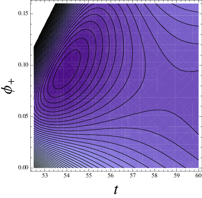
The minima we found are consistent and (meta)stable provided that the messenger fields, that we assumed to have zero vev, have positive masses. This can be always ensured, by properly choosing the various messenger couplings. On the other hand, the absence of tachyonic modes for the messengers is much weaker than the requirement that the messenger masses are phenomenologically viable. Thus, we postpone the study of the phenomenological bounds on the messenger couplings to the following sections.

4.1.2 Lifetime of the metastable vacuum

In this section we consider the metastability of the vacuum by studying the other possible vacua that can be present in case we allow the messenger fields to get non-zero vev’s. Our aim is to prove that the probability decay is very small, the latter being given, in the semiclassical case and in the triangular approximation [23], by $e^{-S_{b}}$ , $S_{b}=(\Delta\Phi)^{4}/\Delta V$ , with $\Delta\Phi$ the typical variation of the fields in passing from a metastable minimum to a stable one, and $\Delta V$ being the corresponding variation of the potential. We approach this problem in a simplified version, assuming that only one messenger field develops a vev, and we distinguish the three cases in which such a field (i) is neutral (ii) has positive charge, (iii) has negative charge; moreover, we consider here only the rigid SUSY case, neglecting the $T$ -modulus field. This is reasonable since eventual minima in which the position of $T$ varies sensibly are harmless. Indeed, the only problem would be a strong decrease of $T$ , but in such a case we can estimate $\Delta V<e^{-bt}/(2t)^{3}$ , while $\Delta\Phi\sim\Delta t$ . Thus, we have $S_{b}\sim 8e^{bt}(t_{0}-t)^{4}t^{3}$ with $t_{0}\sim 10^{2}$ , and, assuming $t\ll t_{0}$ , $t>1$ , we have $S_{b}\gg 1$ . In a similar way, we can argue that any vacuum displaced from the metastable one by a large change in the other fields is harmless for metastability. Indeed, since all the fields (but $T$ ) enter polynomially in the superpotential, and have canonical kinetic terms, we can argue that $\Delta V\sim W_{0}^{2}/(2t)^{3}$ , thus $S_{b}\sim(\Delta\Phi)^{4}W_{0}^{-2}(2t)^{3}\sim(\Delta\Phi)^{4}10^{30}$ in our case. Thus, in what follows we will consider as dangerous only minima where the field vev’s are very close to the metastable case.

Neutral Messengers

In this case we consider the fields $\phi_{+}$ , $\phi_{-}$ , $M_{(0)}$ , $\widetilde{M}_{(0)}$ having canonical Kähler potential. For these fields we take the superpotential (in the simple case $q=1$ . The more general case $q\not=1$ is similar)

\displaystyle W=m\phi_{+}\phi_{-}+(\lambda_{0}\phi_{+}\phi_{-}+\mu)M_{(0)}\widetilde{M}_{(0)}+\Lambda\phi_{-}\ .

(63)

That is a simplification of the general form given previously, in which we neglect the constant term $W_{0}$ , irrelevant in the rigid case, and we introduce the constant term $\Lambda$ to mimic the term $ae^{-bT}$ . Introducing the D-term potential

V_{D}=\frac{g^{2}}{2}D^{2},\,\,\,D=\phi_{+}^{2}-\phi_{-}^{2}+\xi_{FI}^{2}\ ,

(64)

we can compute the rigid potential. With this at hand we can first check the extremum at zero messenger vev’s, i.e. our metastable minimum. We find

\phi_{-}^{2}\sim\xi_{FI}^{2},\,\,\phi_{+}\sim-\frac{\Lambda}{2m},

(65)

in qualitative agreement with the study described above including all the SUGRA corrections. The obtained $\phi_{+}$ value is only an order of magnitude estimate, but we will see that this is more than enough for our purposes. We can now consider the extra solution in the presence of non-zero messenger vev, looking for solutions “close” to the previous one. In particular, assuming $\phi_{+}\ll\phi_{-}$ and $\phi_{-}^{2}\sim\xi_{FI}^{2}$ , we find that the e.o.m.’s admit a single solution, in the $\mu=0$ limit, for

\phi_{-}^{2}=\xi_{FI}^{2},\,\,\phi_{+}=0,\,\,M_{(0)}\widetilde{M}_{(0)}=-\frac{m}{\lambda_{0}}\ .

(66)

We see that this solution is distinct from the previous one. Therefore, even assuming large SUGRA corrections, we expect $\Delta\phi_{+}\sim\Lambda/m$ , big enough to ensure a long-lived metastable vacuum. This result is stable against perturbations due to the presence of a non-zero $\mu$ , as long as $\mu$ remains small enough. For large $\mu$ , on the other hand, the minimum (66) disappear altogether.

Negative charge messengers

In this case we consider the fields $\phi_{+}$ , $\phi_{-}$ , $M_{(-)}$ , $\widetilde{M}_{(-)}$ having canonical Kähler potential and superpotential

\displaystyle W=m\phi_{+}\phi_{-}+\lambda_{+}\phi_{+}M_{(-)}\widetilde{M}_{(-)}+\Lambda\phi_{-}\ ,

(67)

motivated as above. We took for illustration messenger charges $-1/2$ ; again the result is qualitatively similar for other negative charges. The F- and D-terms are

	$\displaystyle D=\|\phi_{+}\|^{2}-\|\phi_{-}\|^{2}-\frac{1}{2}\|M_{(-)}\|^{2}-\frac{1}{2}\|\widetilde{M}_{(-)}\|^{2}+\xi_{FI}^{2}\ ,\,\,\,\,\,\,$
	$\displaystyle F_{\phi_{+}}=m\phi_{-}+\lambda_{+}M_{(-)}\widetilde{M}_{(-)},\,\,\,\,\,\,F_{\phi_{-}}=m\phi_{+}+\Lambda,$		(68)
	$\displaystyle F_{M_{(-)}}=\lambda_{+}\phi_{+}\widetilde{M}_{(-)},\,\,\,\,\,\,F_{\widetilde{M}_{(-)}}=\lambda_{+}\phi_{+}M_{(-)}.$

In case we neglect the $\Lambda$ corrections, a SUSY minimum is present at $\phi_{+}=0$ , with the vev’s of $\phi_{-}$ and $M_{(-)}$ , $\widetilde{M}_{(-)}$ fixed by the $D=0$ and $F_{\phi_{+}}=0$ conditions. The minimum is actually a one-dimensional flat direction in the $\phi_{-}$ , $M_{(-)}$ , $\widetilde{M}_{(-)}$ space, that can be dangerously close to the metastable minimum only in case the messengers have similar vev’s (if an hierarchy is present, then the value of $\phi_{-}$ is significantly smaller than in the metastable vacuum, and thus we do not expect a fast decay of the latter in the new minimum). We can thus study the most problematic case $M_{(-)}\sim\widetilde{M}_{(-)}=M$ . In this case, fixing $\phi_{-}$ via the F-term condition, we have the requirement

\frac{\lambda_{+}^{2}}{m^{2}}|M|^{4}+|M^{2}|=\xi_{FI}^{2},

(69)

that has solution $M^{2}\sim\xi_{FI}^{2}$ for $\lambda_{+}\ll m$ , and $M^{2}\sim\xi_{FI}m/\lambda_{+}$ for $\lambda_{+}\gg m$ . The first (as well the “intermediate” case $\lambda_{+}\sim m$ ) is harmless, since the new vacuum is “far” from the metastable one. A possible problem may arise in case $\lambda_{+}\gg m$ , since the variation of the messenger fields vev in this case is very small. In such case, we argue that the vev $\phi_{+}$ varies sensibly, such that the new vacuum is “far” enough from the metastable one, that remains long lived. In order to have an estimate of $\phi_{+}$ in the new minimum, we have to introduce the $\Lambda$ corrections that, in the metastable case, lead to $\phi_{+}\sim-\Lambda/2m$ . In the present case we can use the e.o.m. and observe that, in the approximation $\lambda_{+}\gg m$ , $\phi_{+}$ is stabilized at values much smaller than $\Lambda/2m$ . In other words, $\phi_{+}$ is stabilized due to a different mechanism then before. Indeed, in the presence of a non-zero messenger vev, we observe a tension between the $F_{\phi_{-}}=0$ and the $F_{M_{-}}=0$ conditions, not present in the metastable case, that pushes $\phi_{+}$ to smaller values. Thus, we expect this solution for $\phi_{+}$ to be distinct from the metastable solution, even when considering the whole SUGRA potential, so that $\Delta\phi_{+}\sim\Lambda/m$ , big enough to ensure the metastable minimum to be long lived.

Positive charge messengers

In this case it was checked in [4] that no dangerous new vacua are present. This provides an interesting example of a messenger sector that introduces no dangerous minimum breaking charge/color. On the other hand, that model does not realizes a standard GMSB transmission, but a combination of gravity and non-standard gauge contributions.

4.1.3 Constraints and assumptions for messengers

Important constraints have to be imposed on the messengers sector from consistency requirements of the theory, but also from a phenomenological point of view. These constraints concern in particular the number of the messengers, the relation between their relative charges and their couplings to the supersymmetry breaking fields $\Phi_{+}$ and $\Phi_{-}$ .
As discussed above, the only constraints on the numbers and charges of messengers coming from the anomalies, is determined by the relation

\Sigma_{i=1}^{N_{+}}n_{i}-\Sigma_{j=1}^{N_{-}}m_{j}=c\ ,

(70)

where $c$ is dictated by the peculiar expressions for the gauge kinetic functions . Therefore, in particular, in the simplest case where all the charges are $\left(\pm q\right)$ and $c>0$ , the relation (70) is translated in $N_{+}-N_{-}>0$ .
Nonetheless, it is well known [1] that whereas the presence of messenger fields at an intermediate scale does not modify the value of $M_{GUT}$ , the inverse gauge coupling strength at the unification scale $M_{GUT}$ receives extra contributions

\delta\alpha_{GUT}^{-1}=-\frac{N}{2\pi}\log{\left(\frac{M_{GUT}}{m_{f}}\right)}\ ,

(71)

with $N$ the number of messengers (when all of them are in the fundamental representation of $SU(5)$ ) and $m_{f}$ their supersymmetric (fermionic) mass. Therefore there is an upper bound on the total number of messengers given by the request of perturbativity of gauge interaction up to the cutoff scale of the model, and depending on their mass scale. Thus a conservative choice is

(N_{+}+N_{-}+N_{0})\log{\left(\frac{M_{P}}{m_{f}}\right)}<150\ ,

(72)

in the approximation that all the messengers are at the same scale $m_{f}$ . Moreover, this is also a necessary condition in order to be able to do a phenomenological numerical analysis. In fact, if some messengers appear at low-energy scale, and others at high-energy, the dynamics at intermediate scale is governed not only by the MSSM fields, but also by the low-energy messengers. This complicate the RG flow equations of the theory and makes the model difficult to study, since the precise results really f depend on the details of the model. Therefore, for simplicity, during our analysis we assumed all the messengers having in first approximation the same high-energy supersymmetric mass (of the order of the GUT scale), since in this way they do not change the RG flow equations for soft terms.
However it is useful to discuss in any case the limits on the couplings $\lambda$ . Referring to the minimization procedure in the case $p=0$ , we can write the conditions that couplings, or equivalently, the supersymmetric masses have to satisfy in order to keep the minimum stable and do not introduce tachyonic directions. This condition comes from requiring positive eigenvalues for the mass scalar matrix (43).
It is easy to see that for the messengers with positive $U(1)_{X}$ charges, the eigenvalues are automatically positive once reasonable charges are imposed.
The conditions for the negatively charged and neutral messengers read instead

	$\displaystyle(m_{f})_{j}=\lambda_{(-)j}\|\Phi_{+}\|^{m_{j}}$	$\displaystyle>$	$\displaystyle\sqrt{3}m_{j}\|\Phi_{+}\|^{-1}\left(1+\frac{\|\Phi_{+}\|}{2\sqrt{3}m_{j}}\right)m_{3/2}\simeq 10^{2}m_{j}m_{3/2}$		(73)
	$\displaystyle(m_{f})_{r}=\lambda_{(0)r}\|\Phi_{+}\Phi_{-}\|^{l_{r}}c_{r}$	$\displaystyle>$	$\displaystyle l_{r}\left(\left\|\frac{F_{+}}{\Phi_{+}}+\frac{F_{-}}{\Phi_{-}}\right\|\right)\simeq 10^{2}l_{r}m_{3/2}\ .$		(74)

Therefore, the limits imposed by consistency are not stronger than those imposed by phenomenology, which require messengers much heavier than the electroweak scale.
Finally, as introduced at the beginning of the section, we could in principle add to the superpotential (55) terms of the form $\left[\lambda\left(\Phi_{+}\Phi_{-}\right)^{k}-\mu\right]\left(a_{1}M_{-}\tilde{M}_{+}+a_{2}M_{+}\tilde{M}_{-}\right)$ , if there exists two couples of messengers with opposite $U(1)_{X}$ charge. Once diagonalized the mass matrix for $M_{+},M_{-},\tilde{M}_{+}\tilde{M}_{-}$ , it is possible to see that the picture is similar to that of the neutral messengers, with the introduction of effective parameters like $c_{r}$ taking into account sums and differences of masses. However in this case the masses are naturally of the same order, or in other words these effective parameters $c_{r}$ can be very small and generate tachyonic directions. The final result should then depend on the details of the model. Therefore, in what follows we will forbid these terms for simplicity.

5 Phenomenological consequences

In what follows we investigate the effects of supersymmetry breaking in the observable sector, that we take to be the Minimal Supersymmetric Standard Model (MSSM). As introduced above, the model described by the superpotential (55) modifies in a non trivial way the results already obtained in [4], due to the presence of the messengers with opposite and neutral charges. However, the main feature of the hybrid model is preserved: gravity and gauge mediation give comparable contributions to the soft terms. The non–universality in the scalar sector induced by gauge mediation, and the negative non–standard contribution induced by D–terms have severe consequences on the mass spectrum and relic density constraints.

5.1 General parameterization of Hybrid Models

The different contribution from the three mediation mechanisms (standard gauge, non-standard gauge and gravity, see the Appendix for details) can be parameterized by the gravitino mass $m_{3/2}$ , and two dimensionless parameters $\alpha$ (defined in Eq. (11)) and $\beta$ which measure the relative size of standard and non-standard gauge mediation contributions with respect to $m_{3/2}$ ; by introducing them, we disentangle the microscopic description of a hybrid model, given in Sect. 4, from its phenomenological study. We can then write the breaking terms:

	$\displaystyle M_{a}$	$\displaystyle=$	$\displaystyle m_{3/2}\left(\tilde{\epsilon}+g^{2}_{a}S_{Q}~\alpha\right)$
	$\displaystyle m_{i}^{2}$	$\displaystyle=$	$\displaystyle m_{0}^{2}+m_{3/2}^{2}C_{i}S_{Q}\left(-\beta+\frac{\alpha^{2}}{N}\right),$		(75)

where $S_{Q}$ is the Dynkin index of the messenger representation (1/2 for the fundamental representation of $SU(N)$ ), $g^{2}_{a}$ are the gauge couplings and $C_{i}=\sum_{a}g^{4}_{a}C^{a}_{i}$ , $C^{a}_{i}$ being the Casimir of the MSSM scalar fields representations (in our normalization the Casimir of the fundamental representation of $SU(N)$ is $(N^{2}-1)/(2N)$ , that of $U(1)_{Y}$ is simply $Y^{2}$ ). The gravitational contribution for the scalar fields is indicated here as $m_{0}^{2}$ , but it will be taken equal to $m_{3/2}^{2}$ in our analysis. The extra parameter $\tilde{\epsilon}$ includes the effects of gravity mediation for gauginos. Whereas the coefficient relating $m_{0}^{2}$ and $m_{3/2}^{2}$ is of order 1, we will see in the following that $\tilde{\epsilon}$ is instead of order ${\cal O}(10^{-1})$ . $N$ is the “effective” number of messenger fields contributing to GMSB. Unlike the classical GMSB at low energy, the mediation in the hybrid models occur around the GUT scale where the gauge contributions to the gaugino masses $M_{a}$ (proportional to their gauge couplings $g_{a}$ ) are approximately universal. Thus, the non-universality only affects the scalars masses. Concerning the trilinear couplings $A_{i=t,b,\tau}$ , there is no 1-loop messenger contribution to the susy-breaking trilinear terms. However $A_{i}$ terms are generated in the leading log approximation by the RG evolution and are proportional to gaugino masses. At GUT scale we will make no assumption on the value of the trilinear couplings. They will be considered as free parameters thorough the phenomenological study. The reader can find in the appendix the explicit expression of the mass terms for each generation of squarks and sleptons.

5.2 Link with microscopic models

The parametrization of eq. 75, and in particular the allowed values for the parameters therein, is the main information with phenomenological relevance we extract from any microscopic construction.

In the high-energy model defined by the superpotential (55), after the minimization procedure shown in the section (4.1.1), in the first approximation it is possible to express all these low-energy parameters in terms of $m_{3/2}$ and the messengers masses and charges.
In a simplified case, where all the subleading contributions are neglected, all the messengers are taken at the same mass scale $m_{mess}$ and couplings $\lambda_{i}$ , all the charges $n_{i},m_{j},l_{r}=1$ , the mass parameter $\mu_{r}=0$ and, as before, $p=0$ , the correspondence is

$\displaystyle\tilde{\epsilon}$	$\displaystyle\simeq$	$\displaystyle\frac{(4+3q)}{2}\left[\log{\left(\frac{1}{m_{3/2}}\right)}+\kappa\right]^{-1}\ ,$
$\displaystyle N$	$\displaystyle\simeq$	$\displaystyle N_{-}+N_{0}\ ,$
$\displaystyle\alpha$	$\displaystyle\simeq$	$\displaystyle\frac{\sqrt{3}N}{8\pi^{2}}\frac{1}{\langle\phi_{+}\rangle}\ \simeq\ \frac{N}{4\pi^{2}~q}\left[\log{\left(\frac{1}{m_{3/2}}\right)}+\kappa\right]\ ,$
$\displaystyle-\beta$	$\displaystyle\simeq$	$\displaystyle\frac{3}{(8\pi^{2})^{2}}\frac{1}{\langle\phi_{-}\rangle^{2}}c\left[1-\log{\left(\frac{\Lambda_{UV}^{2}}{m_{mess}^{2}}\right)}\right]$	(76)
	$\displaystyle\simeq$	$\displaystyle\frac{1}{32\pi^{4}~q}\left[\log{\left(\frac{1}{m_{3/2}}\right)}+\kappa\right]c\left[1-\log{\left(\frac{\Lambda_{UV}^{2}}{m_{mess}^{2}}\right)}\right]\ ,$	(76)

where anomaly cancellation fixes $c\simeq N_{+}-N_{-}$ , $c$ having been defined in eq. 54, and the SUSY breaking field $S$ has been identified with $\phi_{+}$ . Moreover, $\beta$ can be positive of negative; in what follows we consider the most interesting case $\beta>0$ . Finally, $\kappa$ is an ${\cal O}(1)$ parameter. The qualitative picture does not change much in the most general case. Nonetheless in this approximation we can estimate a reasonable range of values for these parameters in our phenomenological analysis, imposing some constraint required by consistency, coming for example from the link between the gravitino mass and $\alpha$ and $\beta$ , or the constraints on the numbers of messengers as discussed in section (4.1.3), depending on their mass.

In the models of Sections 4,5 $\alpha$ can vary between 0 and ${\mathcal{O}}(100)$ , $\beta$ can vary between 0 and ${\mathcal{O}}(10)$ . Thus we can describe/motivate a regime where gravity mediation is dominant, one where standard gauge mediation is (marginally) dominant and an intermediate regime where the model is truly hybrid.

5.3 Gravity vs. GMSB

Gauge mediation is dominant either by enlarging the number of messengers (indeed, $\alpha$ grows linearly with N), or by choosing the microscopic parameters to fix the vev’s of the fields with relevant F-term to small values. Moreover, we will consider $\tilde{\epsilon}=10^{-1}$ in all our phenomenological discussion, in a qualitative agreement with the formula given above. It is evident that for $\alpha\sim 0$ , the exact value of $\tilde{\epsilon}$ should be very important for the numerical results.

It is easy to see that in a large region of the parameter space the model is really hybrid, in the sense explained in section 3. In that region, the parameters $\alpha,\beta,N$ and $q$ , are $\sim{\cal O}(1)$ , whereas $\epsilon\sim{\cal O}(10^{-1})$ .

However, it is compelling to check if it is possible to obtain pure gravity or pure standard gauge mediation in some corner of the parameter space.
Actually pure gravity mediation, or something undistinguishable from it, is obtained when the parameters $\alpha$ and $\beta$ are negligible. This happens for example when the total number of messengers is small and in particular $N\sim 0$ . In particular, the example analyzed in [4] flows into this scenario by lowering the number of the positively charged messengers or increasing their mass.

More difficult instead is to obtain pure standard gauge mediation, taking into account the condition (72) and the minimization result $\langle\phi_{+}\rangle=-\xi_{FI}^{2}/\sqrt{3}=\sqrt{3}q/(2bt)$ . The requirements are then $\frac{\alpha^{2}}{N}\gg 1$ but also $\frac{\alpha^{2}}{N}\gg\beta^{2}$ . The following example illustrates the limits we can reach. Take $q=1/5$ , $\tilde{\epsilon}\sim\frac{1}{15}$ and $N=15$ and obtain:

\displaystyle\langle\phi_{+}\rangle\sim\frac{1}{400}\ ,\quad m_{3/2}\sim 100~{\rm GeV}\qquad\alpha\sim 75\qquad\beta\sim 1\ .

(77)

We are allowed to choose $q$ at an apparently unnatural small value (1/5), crucial in order to lower the $\langle\phi_{+}\rangle$ value, interpreting the coupling $e^{-bT}\Phi^{q}$ in the superpotential as coming from the condensation of a strongly coupled sector. In this case in fact, $q\sim\frac{N_{f}}{N_{c}}$ with $N_{f}$ and $N_{c}$ respectively the number of flavors and colors of such a nonperturbative theory [10, 4]. Lowering the value of the gravitino mass acts in the direction of increasing $\alpha$ . However, while $\langle\phi_{+}\rangle$ (and then $\alpha$ ) depends logarithmically on $m_{3/2}$ , the soft terms decrease proportionally to the gravitino mass. Fixed all the other parameters, the phenomenology impose therefore a lower limit for the value for $m_{3/2}$ . The resulting soft terms at high energy are

M_{a}\gtrsim 1~{\rm TeV}\qquad m_{i}^{2}\sim(1~{\rm TeV})^{2}

(78)

Although the gauge to gravity contribution to scalar mass squared is only 100:1, the diagonal entries (in flavor space) in the scalar mass matrix are enhanced by the RG evolution to low energy, making in this way negligible the non-universal terms dangerous for the FCNC problem [24].
However, after a more detailed analysis, described in the rest of this Section, it is possible to see that at low-energy, even if the FCNC problem is reasonably solved in the squarks sector, it is still open in the sleptons one, as shown in Table 1. Finally, another possibility could be to decrease the factor $c_{r}$ coming from the contribution of neutral messengers. For these fields we are in fact allowed to add an explicit mass term $\mu_{r}$ with $\mu_{r}+\lambda_{(0)r}(\Phi_{+}\Phi_{-})^{l_{r}}\ll 1$ , in order to enforce by tuning a light neutral messenger mass. The net effect is the increasing of the gauge mediation contribution coming from this kind of messengers; therefore $\alpha$ grows keeping fixed all the other parameters. However, one has to be careful to not produce tachyonic directions in messengers directions (73), so this possibility need to be investigated in more detail before concluding about its viability.
As last remark, whereas gauge mediation provides a natural solution to the FCNC problem of supersymmetric theories, it has serious problems in generating the right order of magnitudes for the $\mu$ , $B\mu$ mass parameters of MSSM. On the other hand, hybrid models with a moderate gravity contribution ( $m_{3/2}\sim 10-100$ GeV) can provide a viable solution of the $B-\mu$ problem [8, 25].

5.4 Predictions-general discussion

The main prediction of the class of models with anomalous $U(1)_{X}$ symmetry considered in this paper is the existence of a lower bound on the vevs of the fields relevant for supersymmetry breaking of order of $10^{-3}$ in the Planck mass units. This implies an upper bound on the parameter $\alpha$ present in Eq. (75) for the soft superpartner masses. The bound on $\alpha$ also depends on the acceptable number of messengers consistently with the gauge coupling unification. For necessarily heavy messengers N can be even around 20. Both effects together give an upper bound on $\alpha$ of order of 100 and this has important phenomenological consequences.

It is convenient to organize our phenomenological discussion into two cases, depending on weather the LSP is neutralino or gravitino. Indeed, a quick look at Eq. (75) tells us that for $\alpha$ larger than $\sim 8$ , $m_{3/2}\lesssim 2M_{1}\mathrm{(GUT)}$ , implying $m_{3/2}\lesssim M_{1}\mathrm{(EW)}$ : for such values of $\alpha$ , the gravitino is the LSP and the stable relic candidate.

Thus, in the region where neutralino is the LSP (small values of $\alpha$ ), gravity mediation contribution to the soft masses remains important or can even be the dominant one. The sfermion soft masses are then necessarily of the order of the graviton mass and, for instance, the indirect limit on the stop mass following from the experimental lower bound on the higgs mass implies gravitinos in the several hundreds GeV range. However, the new element of models with anomalous $U(1)_{X}$ and messengers is the presence of non-standard gauge mediation contribution to sfermion masses generated by D-terms. As already shown in [4], when gravity and gauge mediation are comparable, they lead to interesting effects in the sfermion spectra. As will be shown below in a couple of concrete examples, the predictions of the model in this parameter range can be fully consistent with all experimental constraints and in particular neutralino is a good dark matter candidate.

For larger values of $\alpha$ gravitino becomes the LSP and the role of gauge mediation is increasing. However, the first important point to notice is that, since there is an upper limit on $\alpha$ , the ratio of soft masses to the gravitino mass remains bounded from above and the mentioned above limits on the stop mass imply a lower limit on the gravitino mass of order 50-100 GeV (the role of the left- right mixing in the stop sector, i.e. of A terms is important here). This is interesting since gravitino LSP in such mass range allows for high reheating temperature, consistent with leptogenesis.

However, important constraints on such scenarios come from the life time of the NLSP, to be consistent with nucleosynthesis. It is know that neutralinos as NLSP are acceptable only if very heavy. Better candidates for NLSP are staus (for a recent discussion see [34] and references therein¹⁰¹⁰ 10 We thank David Cerdeño for pointing out this issue to us.), although the lower bound on their masses is in a TeV range, too. It is clear from Eq. (75) that staus can be NLSP only for sufficiently large N. The question of course is if such values are still consistent with our upper bound for $\alpha$ . A detailed study of the full range of values of $\alpha$ is beyond the scope of this paper. However, as we show below in our third example, the model can account for gravitino LSP with around 100 GeV mass and a stau as NLSP with its mass in the TeV range. To our knowledge, this is a rare example of a microscopic model with such properties.

5.5 Examples

We illustrate the previous qualitative discussion and the phenomenological viability of the model in a few concrete examples.

The soft terms are defined in our parametrization (75) by three free parameters at the GUT scale: the gravitino mass $m_{3/2}$ , the standard gauge to gravity mediation ratio parametrized by $\alpha$ and the non–standard gauge to gravity mediation ratio parametrized by $\beta$ . Moreover, we have to take into account N, the number of messengers, the $\mu$ mass-term and the bilinear $B$ -term. The absolute value of $\mu$ is determined by the minimization condition of the Higgs potential (assuming CP conservation), but its sign is not fixed. Furthermore, instead of $B$ it is more convenient to use the low energy parameter $\tan\beta=\langle H_{2}^{0}\rangle/\langle H_{1}^{0}\rangle$ , which is a function of $B$ and the other parameters. Thus the parameter space for a complete phenomenological study of such a model can be restricted to the following set of five parameters:

m_{3/2}\;,\ \hskip 5.69046pt\ \alpha\;,\ \hskip 5.69046pt\ \beta\;,\ \hskip 5.69046pt\ N\;,\ \hskip 5.69046pt\ \tan\beta\;,\ \hskip 5.69046pt\ {\rm sgn}(\mu)\;.

(79)

In the following we first discuss the constraints we place upon the model. It includes theoretical constraints (electroweak symmetry breaking condition, color and charge breaking minima, dark matter abundance) as well as current bounds from accelerator experiments. Then we present our results.

(i) The mass spectrum constraints:

We have implemented in our analysis the lower bounds on the masses of SUSY particles and of the lightest Higgs boson. In the squark and slepton sector we checked for the occurrence of tachyons. We applied in our analysis the LEP2 lower bound limit on the mass of the lightest chargino $m_{\tilde{\chi}^{+}_{1}}>103.5$ GeV. In the non-tachyonic region, typically, the most constraining is the lightest Higgs boson mass constraint. In the decoupling limit ( $M_{A}\gg M_{Z}$ , applicable in all our parameter space), $m_{h}>113.5$ GeV at $3\sigma$ . This bound is very sensitive to the value of the top mass. We have taken $m_{t}=171$ GeV throughout our analysis.

(ii) The $b\rightarrow s\gamma$ branching ratio:

One observable where SUSY particle contributions might be large is the radiative flavor changing decay $b\rightarrow s\gamma$ . In the Standard Model this decay is mediated by loops containing the charge 2/3 quarks and $W-$ bosons. In SUSY theories additional contributions come from loops involving charginos and stops, or top quarks and charged higgs bosons. The measurements of the inclusive decay $B\rightarrow X_{s}\gamma$ at CLEO [29] and BELLE [30], leads to restrictive bounds on the branching ratio $b\to s\gamma$ . We impose in our analysis $2.33\times 10^{-4}\leq BR(b\to s\gamma)\leq 4.15\times 10^{-4}$ at the 3 $\sigma$ level. Our analysis considers standard model contributions up to the next to leading order (NLO) and takes into consideration the tan $\beta$ enhanced contributions in MSSM beyond the leading order. We mostly choose $\mu>0$ allowing cancelations between chargino and charged Higgs contributions.

(iii) The anomalous moment of the muon:

We have also taken into account the SUSY contributions to the anomalous magnetic moment of the muon, $a_{\mu}=(g_{\mu}-2)/2$ . We used in our analysis the recent experimental results for the muon anomalous magnetic moment [31], as well as the most recent theoretical evaluations of the Standard Model contributions [32]. It is found that when $e^{+}e^{-}$ data are used the experimental excess in $(g_{\mu}-2)$ constrains a possible SUSY contribution to be $7.1\times 10^{-10}\lesssim a^{\rm SUSY}_{\mu}\lesssim 47.1\times 10^{-10}$ at $2\sigma$ level. However when tau data is used a smaller discrepancy with the experimental measurement is found. In order not to exclude the latter possibility, when analyzing the parameter space with $\mu>0$ we will simply plot contours with the relevant value $a^{\rm SUSY}_{\mu}=7.1\times 10^{-10}$ .

(iv) Relic Density:

Our basic assumption is that the LSP is stable on cosmological time scales. Furthermore we will assume that the LSP abundance is thermal. Within such a framework, the regions of the parameter space that lead to overproduction of dark matter are excluded. On the other hand, the regions that yield LSP abundance below the WMAP limit are not considered as excluded (though as less favored), but simply require non–thermal production or a dark matter candidate beyond the soft spectrum. The WMAP collaboration gives the 3 $\sigma$ narrow limit [33]

0.087\raise 1.29167pt\hbox{$\;<$\kern-7.5pt\raise-4.73611pt\hbox{$\sim\;$}}\Omega_{\chi}h^{2}\raise 1.29167pt\hbox{$\;<$\kern-7.5pt\raise-4.73611pt\hbox{$\sim\;$}}0.138

(80)

on the dark matter relic abundance.

We show in table 1 three examples of low-energy spectrum in the case of “standard” hybrid mediation (A), with a non–standard contribution (B) and case (C) of a moderate dominance of gauge mediation based on the example of Eq. (77). The selected points (A) and (B) respect accelerators and WMAP constraint. The example (C) is also consistent with accelerator constraints and the gravitino LSP with 100 GeV mass is a good dark matter candidate for the reheating temperature of order $10^{-8}$ (see [34] and references therein).

The points (A) and (B) are selected from a big sample of points obtained by the following procedure: Once $\tan\beta$ and $sgn(\mu)$ are fixed (positive thorough our study), we scan over the gravitino mass $0<m_{3/2}<2$ TeV and $0<\alpha<10$ . The low energy mass spectrum is calculated using the Fortran package SUSPECT [26] and its routines were described in detail in ref. [27]. The evaluation of the $b\rightarrow s\gamma$ branching ratio, the anomalous moment of the muon and the relic neutralino density is carried out using the routines provided by the program micrOMEGAs [28]

The first remark is that the scalar particles are relatively heavier than the gauginos. This mainly comes from the fact that scalars receive at tree level a gravity-mediated contribution proportional to $m_{3/2}$ , whereas this contribution is suppressed by a factor $\tilde{\epsilon}$ for the gauginos, (Eq.75).

Concerning the influence of the negative non–standard gauge-mediated term, if we compare points (A) and (B) we observe that to obtain a similar amount of relic density, the model (B) requires a heavier gravitino. This comes from the fact that the WMAP constraint is achieved through the coannihilation channel $\chi^{0}_{1}-\tilde{\tau}_{1}$ and gauge-mediated negative contributions acts on $m_{\tilde{\tau}_{L}}$ at GUT scale reducing considerably the $\tilde{\tau}_{1}$ mass at electroweak scale (whereas not acting on the gaugino mass): we need a higher value of $m_{0}$ to obtain $m_{\tilde{\tau}_{1}}\sim\chi^{0}_{1}$ where the coannihilation is efficient. This effect is clearly depicted in Fig. 3 where the parameter space excluded because the lightest stau is the LSP, increases for increasing values of $\beta$ . The cosmological allowed region follows the line $m_{\tilde{\tau}_{1}}\sim\chi^{0}_{1}$ where the coannihilation channel is dominant. We illustrate also the effect in Fig. 4 where we plot the allowed region as function of $\beta$ : the parameter space is almost completely excluded for $\beta\raise 1.29167pt\hbox{$\;>$\kern-7.5pt\raise-4.73611pt\hbox{$\sim\;$}}0.5$ because the $\tilde{\tau}_{1}$ becomes the LSP for any $m_{3/2}\lesssim 3$ TeV.

We also have calculated the mass spectrum for the case of moderate dominance of gauge-mediation (point (C) in table 1). In this case, the 100 GeV gravitino is the LSP. A relatively heavy gravitino is necessary to respect the LEPII limit on the higgs mass. The NLSP is stau and its mass is at the border line of the limits given in [34]. As mentioned earlier, no systematic study has been performed of the parameter range corresponding to gravitino LSP.

We illustrate the influence of the trilinear coupling on the parameter space in Fig. 5, where we reproduce the Fig. 3 except for $A_{0}=0$ at GUT scale. We do not observe any point where the stop is tachyonic at the electroweak scale, but a region where the stop can be the LSP for $\beta=1$ . However, no region of the parameter space respect the LEPII constraint on $m_{h}$ : lower values of $A_{0}$ implies lower radiative corrections to the Higgs mass.

	A	B	C
$\mathrm{m_{0}}$	385	1050	100
$\mathrm{\alpha}$	5	4	75
$\mathrm{\beta}$	0	0.4	1
N	6	6	15
$\tan\beta$	35	35	35
$\mu$	890	1971	2070
$M_{1}$	220	506	840
$m_{\chi^{0}_{1}}$	218	504	830
$m_{\chi^{+}_{1}}$	418	953	1542
$m_{\tilde{g}}$	1207	2524	3943
$m_{h}$	118	124	122
$m_{A}$	792	1716	1996
$m_{\tilde{u}_{1}}$	1213	2500	3484
$m_{\tilde{t}_{1}}$	747	1450	2852
$m_{\tilde{e}_{1}}$	482	1303	865
$m_{\tilde{\tau}_{1}}$	227	504	686
$\Omega\mathrm{h^{2}}$	0.091	0.096	*

Table 1: Sample spectra. All masses are in GeV and

A_{0}=-3m_{0}

6 Conclusions and perspectives

Supersymmetry breaking in models with gauged $U(1)$ symmetries and Green-Schwarz mechanism is naturally realized in string theory [10, 16, 4, 5, 7]. Whereas at first sight, in this framework gravity mediation, gauge mediation or a mixture of the two are equally possible, in this paper we found that the constraints coming from gauge invariance and moduli stabilization are surprisingly strong. In particular we found that explicit realizations of models in which gravity transmission could be highly suppressed compared to the gauge contribution are very difficult to obtain; new supersymmetric vacua within the supergravity regime appear and/or gauge mediation vacua are incompatible with a small value of the cosmological constant. Our results therefore imply that models with strong gauge dominance should probably contain at least two moduli fields charged under the gauge anomalous $U(1)$ symmetries, with a highly-nontrivial dynamics. It is useful to compare the situation to models with no gauged $U(1)$ , where the dynamics is much simpler and all possibilities of supersymmetry breaking transmission are realized. From this viewpoint, the situation is similar to the models of moduli stabilization and uplift of the vacuum energy: whereas models with anomalous $U(1)$ ’s, very natural from string theory perspective, are hardly compatible with a TeV supersymmetry spectrum [35], uplifts with F-terms are naturally compatible with it [36, 4]. On the other hand, models with purely F-term dynamics, with no gauged $U(1)$ constraints of the type we discussed in the present paper, are difficult to realize in string theory.

We generalized a previously proposed model which incorporated all the constraints of gauge invariance and moduli stabilization by considering the most general messenger sector compatible with anomaly cancelation. The resulting model, coupled to MSSM, automatically contains gravity, standard and non-standard gauge contributions, which are roughly of the same order. In some regions of the parameter space, standard gauge contributions can moderately dominate over gravity contributions and correspondingly the FCNC effects are below per-cent level. It is however impossible without severe fine-tunings to suppress further the gravity contributions.

The class of models we consider here is phenomenologically fully viable. They can give either neutralino or gravitino as good dark matter candidate. In the latter case, gravitino is necessarily relatively heavy (50-100 GeV). This is cosmologically interesting since it is consistent with high reheating temperature needed for leptogenesis. The BBN constraints on the NLSP can be satisfied (at least at a qualitative level studied in this paper) by the stau, for number of messengers of order 15.

Acknowledgments

Work partially supported by the CNRS PICS # 2530 and 3059, RTN contracts MRTN-CT-2004-005104 and MRTN-CT-2004-503369 and the European contract MTKD-CT-2005-029466. E.D. and Y.M. would like to thanks the Institute for Theoretical Physics of Warsaw form warm hospitality and financial support via the “Marie Curie Host Fellowship for Transfer of Knowledge” MTKD-CT-2005-029466. Y.M. would like to thank the European Network of Theoretical Astroparticle Physics ILIAS/N6 under contract number RII3-CT-2004-506222 and the French ANR project PHYS@COLCOS for financial support. The work of A.R. and M.T. was supported by the European Commission Marie Curie Intra-European Fellowships under the contract N 041443 and N 041273. The authors thank D. Cerdeño, M. Cvetic, M. Lennek and G. Shiu for useful discussions. E.D., S.P., A.R. and M.T. thank the Theory Group of CERN for hospitality during the completion of this work.

Appendix A Appendix

A.1 Gravity mediation contribution

The scalar mass matrix is defined as

M_{0}^{2}=\begin{array}[]{|cc|}m^{2}_{I\bar{J}}&m^{2}_{IJ}\ ,\\ m^{2}_{\bar{I}\bar{J}}&m^{2}_{\bar{I}J}\end{array}~,

(81)

where the various entries are :

	$\displaystyle m^{2}_{I\bar{J}}=~\langle\partial_{I}\partial_{\bar{J}}V\rangle~=~\langle\nabla_{I}\nabla_{\bar{J}}V\rangle\ ,$		(82)
	$\displaystyle m^{2}_{IJ}=~\langle\partial_{I}\partial_{J}V\rangle~=~\langle\nabla_{I}\nabla_{J}V\rangle\ .$		(83)

The general expressions of the masses, for vanishing vacuum energy, are of the form [16]:

$\displaystyle m^{2}_{I\bar{J}}$	$\displaystyle=$	$\displaystyle e^{G}(G_{I\bar{J}}+\nabla_{I}G^{\bar{K}}\nabla_{\bar{J}}G_{\bar{K}}-R_{I\bar{J}K\bar{L}}G^{K}G^{\bar{L}}~)+{1\over 2}\sum_{A}g_{A}^{2}D_{A}^{2}(G_{\bar{J}}G_{I}-G_{I\bar{J}})$	(84)
	$\displaystyle-$	$\displaystyle\sum_{A}g_{A}^{2}D_{A}(G_{\bar{J}}\partial_{I}D_{A}+G_{I}\partial_{\bar{J}}D_{A}-\partial_{I}\partial_{\bar{J}}D_{A})+\sum_{A}g_{A}^{2}\partial_{I}D_{A}\partial_{\bar{J}}D_{A}\ ,$	(84)
$\displaystyle m^{2}_{IJ}$	$\displaystyle=$	$\displaystyle e^{G}(2\nabla_{J}G_{I}+G^{K}\nabla_{I}\nabla_{J}G_{K})-\sum_{A}g_{A}^{2}D_{A}(G_{J}\partial_{I}D_{A}+G_{I}\partial_{J}D_{A}-\partial_{I}\partial_{J}D_{A})$	(85)
	$\displaystyle-$	$\displaystyle{1\over 2}\sum_{A}g_{A}^{2}D_{A}^{2}(G_{I}G_{J}+\nabla_{I}G_{J})+\sum_{A}g_{A}^{2}\partial_{I}D_{A}\partial_{J}D_{A}\ ,$	(85)

where the function $R_{I\bar{J}K\bar{L}}$ is the Riemann curvature of the Kähler manifold.

The standard results for the soft terms coming from the gravitational effects, depend on some details concerning the coupling of the modulus to the gauge multiplet of the MSSM, and the Kähler potential of the MSSM scalar fields.
From the point of view of a IIB string theory realization, irrespective on which type of brane MSSM sit (D7 or D3 branes), if they contain magnetic fluxes [37] the gauge kinetic functions contain a T-dependence

f_{a}\ =\ {c_{a}\over 4\pi}T\ +\ f_{a}^{(0)}\ ,

(86)

where $c_{a}$ are positive or negative numbers, and $f_{a}^{(0)}$ effective constants generated by the couplings of the MSSM branes to other, stabilized fluxes (e.g. the dilaton $S$ ).
Moreover, by denoting in what follows by $i,j$ matter fields and by greek indices $\alpha$ any field contributing to SUSY breaking, a relevant quantity for computing the soft terms is the coupling of the matter fields metric $K_{i{\bar{j}}}$ to the SUSY breaking fields. For our model in Sections 4 and 5, this can in turn be parameterized as

	$\displaystyle K_{i{\bar{j}}}=(T+\overline{T})^{n_{i}}\left[\delta_{i{\bar{j}}}+(T+\overline{T})^{m_{ij}}\|\phi_{+}\|^{2}Z^{\prime}_{i\overline{j}}+(T+\overline{T})^{p_{ij}}\|\phi_{-}\|^{2}Z^{\prime\prime}_{i\overline{j}}\right.$
	$\displaystyle\left.+(T+\overline{T})^{l_{ij}}(\phi_{+}\phi_{-}Z^{\prime\prime\prime}_{i\overline{j}}+\mathrm{h.c})+O(\|\phi_{i}\|^{4})\right],$		(87)

where $G=K+\log|W|^{2}$ , $K_{i{\bar{j}}}=\partial_{i}\partial_{\bar{j}}K$ , $i$ and $j$ representing the matter fields, not participating to the SUSY breaking mechanism ( $G_{i}=0$ ). The metric $K_{i{\bar{j}}}$ in (87) is written as an expansion in powers of the charged vev fields $\phi_{\pm}/M_{P}\ll 1$ , up to the quadratic order.

Gaugino masses:

The gaugino masses for a general gauge kinetic function $f_{a}$ are given by [38]

M_{a}^{\mathrm{Grav.}}=\frac{\partial_{T}f_{a}}{Re[f_{a}]}e^{K/2}K^{T\overline{T}}D_{T}W\ .

(88)

For the phenomenological analysis, we use the hypothesis of a gauge kinetic function given in (86) and in particular the unified case

\alpha_{a}=\ {c_{a}\over c_{a}+4\pi f_{a}^{(0)}/T}\ \simeq 1\ .

(89)

Under this assumption, using the definitions and the formulas given in the previous sections we obtain

M_{a}^{\mathrm{Grav.}}=m_{3/2}\alpha_{a}\frac{(T+\overline{T})}{3}\ \frac{D_{T}W}{W}=m_{3/2}\alpha_{a}\frac{(T+\overline{T})}{3}\ G_{T}\ \simeq\tilde{\epsilon}~m_{3/2}\ .

(90)

Scalar masses:

Using the classical formulas at the linear order in the D-term [16, 38]

{\tilde{m}}_{0}^{2}|_{i{\bar{j}}}\ =\ m_{3/2}^{2}\left[G_{i{\bar{j}}}-G^{\alpha}G^{\overline{\beta}}R_{i\overline{j}\alpha\overline{\beta}}\right]\ +\ \sum_{a}g_{a}^{2}D_{a}\partial_{i}\partial_{\bar{j}}D_{a}\ ,

(91)

and with the standard definitions

R_{i\overline{j}\alpha\overline{\beta}}\ =\ \partial_{i}\partial_{\overline{j}}G_{\alpha\overline{\beta}}-\Gamma_{i\alpha}^{m}G_{m\overline{n}}\Gamma^{\overline{n}}_{\overline{j}\overline{\beta}}\quad,\quad\Gamma_{i\alpha}^{m}\ =\ G^{m\overline{k}}\partial_{\alpha}G_{i\overline{k}}\ ,

(92)

for the neutral scalar mass terms we obtain, after normalization of the kinetic terms :

	$\displaystyle({\tilde{m}}_{0}^{2})_{i\overline{j}}=m^{2}_{3/2}\left[\delta_{i{\bar{j}}}+\frac{n_{i}}{(T+\overline{T})^{2}}\|G^{T}\|^{2}\delta_{i{\bar{j}}}-\|G^{+}\|^{2}(T+\overline{T})^{m_{ij}+{n_{i}-n_{j}\over 2}}Z^{\prime}_{i\overline{j}}\right.$
	$\displaystyle\left.-\|G^{-}\|^{2}(T+\overline{T})^{p_{ij}+{n_{i}-n_{j}\over 2}}Z^{\prime\prime}_{i\overline{j}}\right]\ .$		(93)

As for the gauginos, for the phenomenological analysis we study in detail the universal case, where the gravity-mediated contributions are dominated by the term

(m_{i}^{\mathrm{Grav.}})^{2}=({\tilde{m}}_{0}^{2})_{i{\bar{j}}}\simeq m_{3/2}^{2}\delta_{i{\bar{j}}}.

(94)

This is actually a strong assumption, since whereas the contribution to the scalar masses coming from the moduli and the field $\Phi_{-}$ are suppressed compared to the universal first term, we have not enough information about the third term in the rhs of (93). Indeed, this term is negligibly small if $r_{ij}\equiv{m_{ij}+{(n_{i}-n_{j})/2}}\leq-1$ , whereas it is comparable to the universal contribution for $r_{ij}=0$ and dominant for $r_{ij}>0$ . Whereas this last case cannot arise in a string compactification, the case $r_{ij}=0$ could and deserve a more detailed study from the viewpoint of possible flavor-dependent $\Phi_{+}$ couplings.

A.2 Standard and Non-standard GMSB contributions

The exact calculation of the radiatively induced gaugino and scalar masses, due to one messenger multiplet, gives [1] for the gaugino mass

M^{\mathrm{GMSB}}_{a}=\frac{g_{a}^{2}m_{f}S_{Q}}{8\pi^{2}}\ \frac{y_{-}\log{y_{-}}-y_{+}\log{y_{+}}-y_{-}y_{+}\log{(y_{-}/y_{+})}}{(y_{-}-1)(y_{+}-1)}

(95)

and for the scalar masses [20, 1]

(m_{i}^{\mathrm{GMSB}})^{2}\ =\ \frac{C_{i}~S_{Q}}{128\pi^{4}}m_{f}^{2}\ F(y_{-},y_{+},\Lambda_{\mathrm{UV}}^{2}/m_{f}^{2})\ ,

(96)

with $y_{i}=m_{i}^{2}/m_{f}^{2}$ and $m_{i},i=\pm$ the two scalar messengers mass eigenvalues. The function $F$ is given by

$\displaystyle F(y_{-},y_{+},\Lambda_{\mathrm{UV}}^{2}/m_{f}^{2})$	$\displaystyle=$	$\displaystyle-(2y_{-}+2y_{+}-4)\log{\frac{\Lambda^{2}_{\mathrm{UV}}}{m_{f}^{2}}}$	(97)
	$\displaystyle+$	$\displaystyle 2(2y_{-}+2y_{+}-4)+(y_{-}+y_{+})\log{y_{-}}\log{y_{+}}$
	$\displaystyle+$	$\displaystyle G(y_{-},y_{+})+G(y_{+},y_{-})\ ,$

where

$\displaystyle G(y_{-},y_{+})$	$\displaystyle=$	$\displaystyle 2y_{-}\log{y_{-}}+(1+y_{-})\log^{2}{y_{-}}-\frac{1}{2}(y_{-}+y_{+})\log^{2}{y_{-}}$	(98)
	$\displaystyle+$	$\displaystyle 2(1-y_{-})\mathrm{Li_{2}}(1-\frac{1}{y_{-}})+2(1+y_{-})\mathrm{Li_{2}}(1-{y_{-}})$
	$\displaystyle-$	$\displaystyle y_{-}\mathrm{Li_{2}}(1-\frac{y_{-}}{y_{+}})\ .$

$\mathrm{Li_{2}}(x)$ refers to the dilogarithmic function, defined by $\mathrm{Li_{2}}(x)=-\int_{0}^{1}dzz^{-1}\log{(1-xz)}$ . If

\lambda F_{S},D\ll\lambda^{2}\langle S\rangle^{2}\ ,

(99)

in (48), then it is easy to see that one can expand the above expressions and have a simplified one in terms of the ratio $\left|\frac{F_{S}}{\langle S\rangle}\right|$ and $D$ . In particular, coming back to our model (55), we can distinguish between the different contributions from the (positively and negatively) charged messengers and the neutral ones. In what follows we will distinguish between the “standard” and the “non-standard” contributions. We give the general result in terms of F-terms and vev’s, and also the approximate result in the case $p=0$ ¹¹¹¹ 11 The case $p>0$ is difficult to study in details, since the lack of analytic formula. Nonetheless, qualitatively it is possible to say that since we expect in that case $\langle\Phi_{+}\rangle\sim\langle\Phi_{-}\rangle$ (whereas for $p=0$ , $\langle\Phi_{+}\rangle\sim 10^{-1}\langle\Phi_{-}\rangle$ ), all the quantities related to the ratio $\frac{\langle\Phi_{-}\rangle}{\langle\Phi_{+}\rangle}$ will decrease by a factor 10. In particular we expect that the standard contributions for the soft masses coming from all the messengers will be of the same order, and moreover smaller by an order of magnitude with respect to the contributions in the case $p=0$ .. For a coupling $\Phi_{-}^{n_{i}^{\prime}}M_{(+)i^{\prime}}\tilde{M}_{(+)i^{\prime}}$ the charge for both the messengers is denoted by $\left(+\frac{n_{i}^{\prime}}{2}\right)$ , whereas for a coupling $\Phi_{-}^{m_{j}^{\prime}}M_{(-)j^{\prime}}\tilde{M}_{(-)j^{\prime}}$ by $\left(-\frac{m_{j}^{\prime}}{2}\right)$ .

Messengers with positive charge:

A messenger $i^{\prime}$ contributes with

$\displaystyle M^{\mathrm{GMSB}}_{a}$	$\displaystyle=$	$\displaystyle\frac{g_{a}^{2}S_{Q}}{8\pi^{2}}n_{i^{\prime}}\frac{F_{-}}{\langle\Phi_{-}\rangle}\ \simeq\ \frac{g_{a}^{2}S_{Q}}{8\pi^{2}}n_{i^{\prime}}\ m_{3/2}\ ,$	(100)
$\displaystyle(m_{i}^{\mathrm{GMSB}})^{2}_{{\mathrm{Stand.}}}$	$\displaystyle=$	$\displaystyle\frac{C_{i}S_{Q}}{64\pi^{4}}n_{i^{\prime}}^{2}\left\|\frac{F_{-}}{\langle\Phi_{-}\rangle}\right\|^{2}\simeq\frac{C_{i}S_{Q}}{64\pi^{4}}n_{i^{\prime}}^{2}\ m_{3/2}^{2}\ ,$	(101)
$\displaystyle(m_{i}^{\mathrm{GMSB}})^{2}_{{\mathrm{Non-Stand.}}}$	$\displaystyle=$	$\displaystyle-\frac{C_{i}S_{Q}}{64\pi^{4}}n_{i^{\prime}}\left(g^{2}_{X}D\right)\left[\log{\left(\frac{\Lambda_{UV}^{2}}{(m_{f})_{i^{\prime}}^{2}}\right)}-1\right]$
	$\displaystyle\simeq$	$\displaystyle-\frac{C_{i}S_{Q}}{32\pi^{4}}n_{i^{\prime}}^{2}\frac{m_{3/2}^{2}}{q}\left[\log{\left(\frac{1}{m_{3/2}}\right)}+\kappa\right]\left[\log{\left(\frac{\Lambda_{UV}^{2}}{(m_{f})_{i^{\prime}}^{2}}\right)}-1\right]\ ,$

where the fermionic mass is given by $(m_{f})_{i^{\prime}}^{2}\simeq\lambda^{2}_{(+)i^{\prime}}\left(\frac{3q}{2}\right)^{n_{i^{\prime}}}\left[\log{\left(\frac{1}{m_{3/2}}\right)}+\kappa\right]^{-n_{i^{\prime}}}$ .

Messengers with negative charge:

A messenger $j^{\prime}$ contributes with

$\displaystyle M^{\mathrm{GMSB}}_{a}$	$\displaystyle=$	$\displaystyle\frac{g_{a}^{2}S_{Q}}{8\pi^{2}}m_{j^{\prime}}\frac{F_{+}}{\langle\Phi_{+}\rangle}\simeq\frac{g_{a}^{2}S_{Q}}{4\pi^{2}}n_{i^{\prime}}\frac{m_{3/2}}{q}\left[\log{\left(\frac{1}{m_{3/2}}\right)}+\kappa\right]$	(103)
$\displaystyle(m_{i}^{\mathrm{GMSB}})^{2}_{{\mathrm{Stand.}}}$	$\displaystyle=$	$\displaystyle\frac{C_{i}S_{Q}}{64\pi^{4}}m_{j^{\prime}}^{2}\left\|\frac{F_{+}}{\langle\Phi_{+}\rangle}\right\|^{2}\simeq\frac{C_{i}S_{Q}}{16\pi^{4}}n_{i^{\prime}}^{2}\frac{m_{3/2}^{2}}{q^{2}}\left[\log{\left(\frac{1}{m_{3/2}}\right)}+\kappa\right]^{2}$	(104)
$\displaystyle(m_{i}^{\mathrm{GMSB}})^{2}_{{\mathrm{Non-Stand.}}}$	$\displaystyle=$	$\displaystyle\frac{C_{i}S_{Q}}{64\pi^{4}}m_{j^{\prime}}\left(g^{2}_{X}D\right)\left[\log{\left(\frac{\Lambda_{UV}^{2}}{(m_{f})_{j^{\prime}}^{2}}\right)}-1\right]$
	$\displaystyle\simeq$	$\displaystyle\frac{C_{i}S_{Q}}{32\pi^{4}}m_{j^{\prime}}^{2}\frac{m_{3/2}^{2}}{q}\left[\log{\left(\frac{1}{m_{3/2}}\right)}+\kappa\right]\left[\log{\left(\frac{\Lambda_{UV}^{2}}{(m_{f})_{j^{\prime}}^{2}}\right)}-1\right]\ ,$

where the fermionic mass is given by $(m_{f})_{j^{\prime}}^{2}\simeq\lambda^{2}_{(-)j^{\prime}}\frac{1}{3}\left(\frac{3q}{2}\right)^{2m_{j^{\prime}}}\left[\log{\left(\frac{1}{m_{3/2}}\right)}+\kappa\right]^{-2m_{j^{\prime}}}$ .

Messengers with zero charge:

A messenger $r^{\prime}$ contributes with

$\displaystyle M^{\mathrm{GMSB}}_{a}$	$\displaystyle=$	$\displaystyle\frac{g_{a}^{2}S_{Q}}{8\pi^{2}}l_{r^{\prime}}c_{r^{\prime}}\left(\frac{F_{+}}{\langle\Phi_{+}\rangle}+\frac{F_{-}}{\langle\Phi_{-}\rangle}\right)$	(106)
	$\displaystyle\simeq$	$\displaystyle\frac{g_{a}^{2}S_{Q}}{4\pi^{2}}l_{r^{\prime}}c_{r^{\prime}}\frac{m_{3/2}}{q}\left[\log{\left(\frac{1}{m_{3/2}}\right)}+\kappa+\frac{q}{2}\right]\ ,$	(106)
$\displaystyle(m_{i}^{\mathrm{GMSB}})^{2}_{{\mathrm{Stand.}}}$	$\displaystyle=$	$\displaystyle\frac{C_{i}S_{Q}}{64\pi^{4}}l_{r^{\prime}}^{2}c_{r^{\prime}}^{2}\left(\left\|\frac{F_{+}}{\langle\Phi_{+}\rangle}+\frac{F_{-}}{\langle\Phi_{-}\rangle}\right\|\right)^{2}$	(107)
	$\displaystyle\simeq$	$\displaystyle\frac{C_{i}S_{Q}}{16\pi^{4}}l_{r^{\prime}}^{2}c_{r^{\prime}}^{2}\frac{m_{3/2}^{2}}{q^{2}}\left[\log{\left(\frac{1}{m_{3/2}}\right)}+\kappa+\frac{q}{2}\right]^{2}\ ,$	(107)

where $c_{r^{\prime}}=\left[1+\frac{\mu_{r^{\prime}}}{\lambda_{0r^{\prime}}\left(\Phi_{+}\Phi_{-}\right)^{l_{r^{\prime}}}}\right]^{-1}$ .
In this case there is no non-standard contribution for the scalar soft masses, since the supertrace for these messengers vanishes.

A.3 Anomaly mediation contributions

The contributions to the terms soft coming from the anomaly mediation mechanism, are typically of order

m^{Anom.}_{i}\sim\frac{g^{2}}{16\pi^{2}}m_{3/2}

(108)

and then are naturally suppressed in our case already by the universal terms coming from the gravity mediation mechanism for $\tilde{\epsilon}\gtrsim{\cal O}\left(10^{-1}\right)$ .
It is interesting to note that this is different from the scenario studied in [13] where the gravity mediation contributions are suppressed with respect to the gravitino mass by a loop factor, and then become of the same order of those produced by anomaly mediation, allowing the so-called mirage unification.

A.4 Explicit soft terms

We explicit in the appendix the charge dependence of the soft breaking terms at high scale for the scalar fields, in the framework of our phenomenological parametrization.

$\displaystyle m_{Q_{L}}^{2}$	$\displaystyle=$	$\displaystyle m_{3/2}^{2}\left\{1+S_{Q}\left(-\beta+\frac{\alpha^{2}}{N}\right)\left[\frac{4}{3}g_{3}^{4}+\frac{3}{4}g_{2}^{4}+\frac{3}{5}\left(\frac{1}{6}\right)^{2}g_{1}^{4}\right]\right\},$
$\displaystyle m_{U_{R}}^{2}$	$\displaystyle=$	$\displaystyle m_{3/2}^{2}\left\{1+S_{Q}\left(-\beta+\frac{\alpha^{2}}{N}\right)\left[\frac{4}{3}g_{3}^{4}+\frac{3}{5}\left(\frac{-2}{3}\right)^{2}g_{1}^{4}\right]\right\},$
$\displaystyle m_{D_{R}}^{2}$	$\displaystyle=$	$\displaystyle m_{3/2}^{2}\left\{1+S_{Q}\left(-\beta+\frac{\alpha^{2}}{N}\right)\left[\frac{4}{3}g_{3}^{4}+\frac{3}{5}\left(\frac{1}{3}\right)^{2}g_{1}^{4}\right]\right\},$
$\displaystyle m_{E_{L}}^{2}$	$\displaystyle=$	$\displaystyle m_{3/2}^{2}\left\{1+S_{Q}\left(-\beta+\frac{\alpha^{2}}{N}\right)\left[+\frac{3}{4}g_{2}^{4}+\frac{3}{5}\left(\frac{-1}{2}\right)^{2}g_{1}^{4}\right]\right\},$
$\displaystyle m_{E_{R}}^{2}$	$\displaystyle=$	$\displaystyle m_{3/2}^{2}\left\{1+S_{Q}\left(-\beta+\frac{\alpha^{2}}{N}\right)\left[\frac{3}{5}\left(1\right)^{2}g_{1}^{4}\right]\right\},$
$\displaystyle m_{H_{u}}^{2}$	$\displaystyle=$	$\displaystyle m_{3/2}^{2}\left\{1+S_{Q}\left(-\beta+\frac{\alpha^{2}}{N}\right)\left[\frac{3}{4}g_{2}^{4}+\frac{3}{5}\left(\frac{1}{2}\right)^{2}g_{1}^{4}\right]\right\},$
$\displaystyle m_{H_{d}}^{2}$	$\displaystyle=$	$\displaystyle m_{3/2}^{2}\left\{1+S_{Q}\left(-\beta+\frac{\alpha^{2}}{N}\right)\left[\frac{3}{4}g_{2}^{4}+\frac{3}{5}\left(\frac{-1}{2}\right)^{2}g_{1}^{4}\right]\right\},$	(109)

where as usual $S_{Q}$ is the Dynkin index of the messenger representation ( $S_{Q}=1/2$ for the fundamental representation), $g_{i}$ are the gauge couplings at GUT scale ( $\alpha_{i}=g_{i}^{2}/16\pi^{2}$ ) whereas $\alpha$ , $\beta$ and $N$ have been defined in Sections 4 and 5. In all our discussion we assumed for simplicity the messengers in complete representations of $SU(5)$ .

References

[1] For a review and extensive references, see e.g. G. F. Giudice and R. Rattazzi, Phys. Rept. 322 (1999) 419 [arXiv:hep-ph/9801271].
[2] D. E. Diaconescu, B. Florea, S. Kachru and P. Svrcek, JHEP 0602 (2006) 020 [arXiv:hep-th/0512170].
[3] O. Aharony, S. Kachru and E. Silverstein, Phys. Rev. D 76 (2007) 126009 [arXiv:0708.0493 [hep-th]] ;
[4] E. Dudas, Y. Mambrini, S. Pokorski and A. Romagnoni, JHEP 0804 (2008) 015 [arXiv:0711.4934 [hep-th]].
[5] M. Cvetic and T. Weigand, arXiv:0807.3953 [hep-th] .
[6] J. J. Heckman, J. Marsano, N. Saulina, S. Schafer-Nameki and C. Vafa, arXiv:0808.1286 [hep-th].
[7] J. J. Heckman and C. Vafa, arXiv:0809.1098 [hep-th].
[8] M. Ibe and R. Kitano, JHEP 0708 (2007) 016 [arXiv:0705.3686 [hep-ph]]; Y. Nomura and M. Papucci, Phys. Lett. B 661 (2008) 145 [arXiv:0709.4060 [hep-ph]]; J. L. Feng, C. G. Lester, Y. Nir and Y. Shadmi, arXiv:0712.0674 [hep-ph]; L. L. Everett, I. W. Kim, P. Ouyang and K. M. Zurek, arXiv:0804.0592 [hep-ph] ; E. Dudas, S. Lavignac and J. Parmentier, arXiv:0808.0562 [hep-ph] ; N. J. Craig and D. Green, arXiv:0808.1097 [hep-ph]. S. Shirai, F. Takahashi, T. T. Yanagida and K. Yonekura, arXiv:0808.0848 [hep-ph]. K. Choi, arXiv:0809.3301 [hep-ph].
[9] Z. Lalak, S. Pokorski and K. Turzynski, arXiv:0808.0470 [hep-ph] ;
[10] P. Binetruy and E. Dudas, Phys. Lett. B 389 (1996) 503 [arXiv:hep-th/9607172]; N. Arkani-Hamed, M. Dine and S. P. Martin, Phys. Lett. B 431 (1998) 329 [arXiv:hep-ph/9803432].
[11] L. Randall and R. Sundrum, Nucl. Phys. B 557 (1999) 79 [arXiv:hep-th/9810155]; G. F. Giudice, M. A. Luty, H. Murayama and R. Rattazzi, JHEP 9812 (1998) 027 [arXiv:hep-ph/9810442].
[12] D. E. Kaplan, G. D. Kribs and M. Schmaltz, Phys. Rev. D 62 (2000) 035010 [arXiv:hep-ph/9911293]; Z. Chacko, M. A. Luty, A. E. Nelson and E. Ponton, JHEP 0001 (2000) 003 [arXiv:hep-ph/9911323].
[13] K. Choi, A. Falkowski, H. P. Nilles, M. Olechowski and S. Pokorski, JHEP 0411 (2004) 076 [arXiv:hep-th/0411066]; K. Choi, A. Falkowski, H. P. Nilles and M. Olechowski, Nucl. Phys. B 718 (2005) 113 [arXiv:hep-th/0503216]; M. Endo, M. Yamaguchi and K. Yoshioka, Phys. Rev. D 72 (2005) 015004 [arXiv:hep-ph/0504036]; A. Falkowski, O. Lebedev and Y. Mambrini, JHEP 0511 (2005) 034 [arXiv:hep-ph/0507110]; K. Choi, K. S. Jeong, T. Kobayashi and K. i. Okumura, Phys. Lett. B 633 (2006) 355 [arXiv:hep-ph/0508029]; O. Lebedev, H. P. Nilles and M. Ratz, Phys. Lett. B 636 (2006) 126 [arXiv:hep-th/0603047].
[14] P. Fayet and J. Iliopoulos, Phys. Lett. B 51 (1974) 461.
[15] L. O’Raifeartaigh, Nucl. Phys. B 96 (1975) 331.
[16] E. Dudas and S. K. Vempati, Nucl. Phys. B 727, 139 (2005) [arXiv:hep-th/0506172].
[17] R. Blumenhagen, M. Cvetic and T. Weigand, Nucl. Phys. B 771 (2007) 113 [arXiv:hep-th/0609191] ; L. E. Ibanez and A. M. Uranga, JHEP 0703 (2007) 052 [arXiv:hep-th/0609213].
[18] S. Kachru, R. Kallosh, A. Linde and S. P. Trivedi, Phys. Rev. D 68 (2003) 046005 [arXiv:hep-th/0301240].
[19] M. Dine, A. E. Nelson and Y. Shirman, Phys. Rev. D 51 (1995) 1362 [arXiv:hep-ph/9408384]; M. Dine, A. E. Nelson, Y. Nir and Y. Shirman, Phys. Rev. D 53 (1996) 2658 [arXiv:hep-ph/9507378].
[20] N. Arkani-Hamed, J. March-Russell and H. Murayama, Nucl. Phys. B 509 (1998) 3 [arXiv:hep-ph/9701286]; E. Poppitz and S. P. Trivedi, Phys. Lett. B 401 (1997) 38 [arXiv:hep-ph/9703246].
[21] G. R. Dvali and A. Pomarol, Phys. Rev. Lett. 77 (1996) 3728 [arXiv:hep-ph/9607383] ; A. G. Cohen, D. B. Kaplan and A. E. Nelson, Phys. Lett. B 388 (1996) 588 [arXiv:hep-ph/9607394] .
[22] N. Arkani-Hamed and H. Murayama, Phys. Rev. D 56 (1997) 6733 [arXiv:hep-ph/9703259].
[23] M. J. Duncan and L. G. Jensen, Phys. Lett. B 291 (1992) 109.
[24] M. Ciuchini, A. Masiero, P. Paradisi, L. Silvestrini, S. K. Vempati and O. Vives, arXiv:hep-ph/0702144.
[25] G. F. Giudice and A. Masiero, Phys. Lett. B 206 (1988) 480.
[26] A. Djouadi, J. L. Kneur and G. Moultaka, Comput. Phys. Commun. 176 (2007) 426 [arXiv:hep-ph/0211331]; see also the web page http://www.lpm.univ-montp2.fr:6714/˜kneur/suspect.html
[27] A. Djouadi, M. Drees and J.L. Kneur, JHEP 0108, 055 (2001), hep-ph/0107316
[28] G. Belanger, F. Boudjema, A. Pukhov and A. Semenov, Comput. Phys. Commun. 149 (2002) 103 [arXiv:hep-ph/0112278]; Comput. Phys. Commun. 174 (2006) 577 [arXiv:hep-ph/0405253]; Comput. Phys. Commun. 176 (2007) 367 [arXiv:hep-ph/0607059].
[29] CLEO Collaboration, S. Chen et al., Phys. Rev. Lett. 87 (2001) 251807 [arXiv:hep-ex/0108032].
[30] BELLE Collaboration, H. Tajima, Int. J. Mod. Phys. A17 (2002) 2967 [arXiv:hep-ex/0111037].
[31] Muon g-2 Collaboration, G. W. Bennett et al., Phys. Rev. Lett. 92 (2004) 161802 [arXiv:hep-ex/0401008].
[32] M. Davier, S. Eidelman, A. Hocker and Z. Zhang, Eur. Phys. J. C 31 (2003) 503 [arXiv:hep-ph/0308213]; K. Hagiwara, A. D. Martin, D. Nomura and T. Teubner, Phys. Rev. D69 (2004) 093003 [arXiv:hep-ph/0312250]; J. F. de Troconiz and F. J. Yndurain, Phys. Rev. D 71 (2005) 073008 [arXiv:hep-ph/0402285];
[33] C. L. Bennett et al. [WMAP Collaboration], Astrophys. J. Suppl. 148 (2003) 1 [arXiv:astro-ph/0302207] D. N. Spergel et al. [WMAP Collaboration], Astrophys. J. Suppl. 148 (2003) 175 [arXiv:astro-ph/0302209]; L. Verde et al. [WMAP Collaboration], Astrophys. J. Suppl. 148 (2003) 195 [arXiv:astro-ph/0302218].
[34] F. D. Steffen, arXiv:0711.1240 [hep-ph] ; D. G. Cerdeno, K. Y. Choi, K. Jedamzik, L. Roszkowski and R. Ruiz de Austri, JCAP 0606 (2006) 005 [arXiv:hep-ph/0509275].
[35] A. Achucarro, B. de Carlos, J. A. Casas and L. Doplicher, JHEP 0606 (2006) 014 [arXiv:hep-th/0601190] ; K. Choi and K. S. Jeong, JHEP 0608 (2006) 007 [arXiv:hep-th/0605108] ; E. Dudas and Y. Mambrini, JHEP 0610 (2006) 044 [arXiv:hep-th/0607077].
[36] M. Gomez-Reino and C. A. Scrucca, JHEP 0605 (2006) 015 [arXiv:hep-th/0602246]; O. Lebedev, H. P. Nilles, and M. Ratz, Phys. Lett. B636 (2006), 126, [hep-th/0603047] ; F. Brummer, A. Hebecker and M. Trapletti, Nucl. Phys. B 755 (2006) 186 [arXiv:hep-th/0605232] ; E. Dudas, C. Papineau and S. Pokorski, JHEP 0702 (2007) 028 [arXiv:hep-th/0610297] ; H. Abe, T. Higaki, T. Kobayashi and Y. Omura, Phys. Rev. D 75 (2007) 025019 [arXiv:hep-th/0611024] ; R. Kallosh and A. Linde, JHEP 0702 (2007) 002 [arXiv:hep-th/0611183] ; O. Lebedev, V. Lowen, Y. Mambrini, H. P. Nilles and M. Ratz, JHEP 0702 (2007) 063 [arXiv:hep-ph/0612035] ; D. Gallego and M. Serone, JHEP 0808 (2008) 025 [arXiv:0807.0190 [hep-th]].
[37] R. Blumenhagen, L. Goerlich, B. Kors and D. Lust, JHEP 0010 (2000) 006 [arXiv:hep-th/0007024]; C. Angelantonj, I. Antoniadis, E. Dudas and A. Sagnotti, Phys. Lett. B 489 (2000) 223 [arXiv:hep-th/0007090].
[38] V. S. Kaplunovsky and J. Louis, Phys. Lett. B 306 (1993) 269 [arXiv:hep-th/9303040] ; A. Brignole, L. E. Ibanez and C. Munoz, Nucl. Phys. B 422 (1994) 125 [Erratum-ibid. B 436 (1995) 747] [arXiv:hep-ph/9308271] ; S. Ferrara, C. Kounnas and F. Zwirner, Nucl. Phys. B 429 (1994) 589 [Erratum-ibid. B 433 (1995) 255] [arXiv:hep-th/9405188].

$\displaystyle V$	$\displaystyle=$	$\displaystyle\frac{e^{-2bt}}{(2t)^{3}}\left[\frac{1}{3}\left\|a(3+2bt)\Phi_{-}^{q}(\Phi_{-}\Phi_{+})^{p}+3e^{bT}(W_{0}+m\Phi_{-}\Phi_{+})\right\|^{2}\right.$	(58)
		$\displaystyle\left.+\left\|a\Phi_{-}^{q-1}(p+q+\|\Phi_{-}\|^{2})(\Phi_{-}\Phi_{+})^{p}+e^{bT}(W_{0}\bar{\Phi}_{-}+m\Phi_{+}(1+\|\Phi_{-}\|^{2}))\right\|^{2}\right.$
		$\displaystyle\left.+\left\|a\Phi_{-}^{q+1}(p+\|\Phi_{+}\|^{2})(\Phi_{-}\Phi_{+})^{p-1}+e^{bT}(W_{0}\bar{\Phi}_{+}+m\Phi_{-}(1+\|\Phi_{+}\|^{2}))\right\|^{2}\right.$
		$\displaystyle\left.-3\left\|e^{bT}\left(W_{0}+m\Phi_{-}\Phi_{+}\right)+a\Phi_{-}^{q}(\Phi_{-}\Phi_{+})^{p}\right\|^{2}\right]+\frac{2\pi}{t}\left(\frac{\xi^{2}}{2t}-\|\Phi_{-}\|^{2}+\|\Phi_{+}\|^{2}\right)^{2}$

Abstract