Systematic Effective Field Theory Investigation of Spiral Phases in Hole-Doped Antiferromagnets on the Honeycomb Lattice
Abstract
Motivated by possible applications to the antiferromagnetic precursor of the high-temperature superconductor NaxCoOyH2O, we use a systematic low-energy effective field theory for magnons and holes to study different phases of doped antiferromagnets on the honeycomb lattice. The effective action contains a leading single-derivative term, similar to the Shraiman-Siggia term in the square lattice case, which gives rise to spirals in the staggered magnetization. Depending on the values of the low-energy parameters, either a homogeneous phase with four or a spiral phase with two filled hole pockets is energetically favored. Unlike in the square lattice case, at leading order the effective action has an accidental continuous spatial rotation symmetry. Consequently, the spiral may point in any direction and is not necessarily aligned with a lattice direction.
pacs
74.20.Mn, 75.30.Ds, 75.50.Ee, 12.39.FeI Introduction
Since the discovery of high-temperature superconductivity in the cuprates [1], identifying the dynamical mechanism behind it remains one of the biggest challenges in condensed matter physics. It has been suggested that the physics of high-temperature superconductivity can be described by --type models. Using a variety of techniques, numerous interesting properties of doped antiferromagnets have been investigated in great detail both numerically and analytically [2, 3, 4, 5, 6, 7, 8, 9, 10, 11, 12, 13, 14, 15, 16, 17, 18, 19, 20, 21, 22, 23, 24, 25, 26, 27, 28, 29, 30, 31, 32, 33, 34, 35, 36, 37, 38, 39]. For instance, as was first pointed out by Shraiman and Siggia [6], a spiral phase with a helical structure in the staggered magnetization is a candidate ground state of doped antiferromagnets even at arbitrarily small doping [10, 18, 21, 23, 24, 25, 26, 27, 28, 30, 31, 34, 36, 35, 37, 38, 40, 41]. Unfortunately, due to the strong electron correlations in these systems, most analytic results suffer from uncontrolled approximations. Similarly, numerical simulations suffer from a severe sign problem away from half-filling. Consequently, although numerous investigations have been devoted to understanding the spiral phases in doped antiferromagnets, some controversial results have been obtained.
In analogy to chiral perturbation theory for the pions in QCD [42, 43], a systematic low-energy effective field theory for the magnons in an antiferromagnet was developed in [8, 9, 12, 44, 22, 29, 33]. Motivated by the success of baryon chiral perturbation theory for pions and nucleons [45, 46, 47, 48, 49], respecting the symmetry constraints of the underlying - model and taking into account the location of the hole or electron pockets in momentum space, low-energy effective field theories for magnons and holes or electrons have been constructed for lightly doped antiferromagnets on the square lattice in [50, 51, 52]. The effective theories are universally applicable and yield results that are exact, order by order in a systematic low-energy expansion. Material-specific properties enter the effective Lagrangian in the form of a priori undetermined low-energy parameters, like the spin stiffness or the spinwave velocity . The effective theories for hole- and electron-doped systems were used to investigate the one-magnon exchange potentials and the resulting two-hole or two-electron bound states as well as possible spiral phases [51, 53, 54, 52]. In the hole-doped case, the leading order magnon-hole coupling is described by the Shraiman-Siggia term that contains just a single spatial derivative. For sufficiently small , even at arbitrarily small hole density, this term stabilizes a zero degree spiral phase in which the spiral is oriented along a lattice axis. In the electron-doped case, on the other hand, the Shraiman-Siggia term is forbidden by the symmetries, and, consequently, spiral phases are not energetically favorable.
In addition to the cuprates, another superconducting material, NaxCoOyH2O [55], has attracted a lot of attention [56, 57, 58, 59, 60, 61]. The underlying triangular lattice of this geometrically frustrated material leads to a severe sign problem and thus prevents us from studying it from first principles using Monte Carlo calculations. On the other hand, the honeycomb lattice structure of the dehydrated variant of NaxCoOyH2O at has motivated several investigations of the antiferromagnetism as well as the single-hole dispersion relation on the non-frustrated honeycomb lattice [62, 63]. In particular, the low-energy parameters of the effective theory for the - model, namely the staggered magnetization [64], the spin-stiffness , the spinwave velocity , and the kinetic mass of a hole have been determined with high precision using an efficient cluster algorithm [63].
Motivated by possible applications to NaxCoOyH2O, using the same methods as for the square lattice [50, 52], we have constructed a systematic effective field theory for the - model on the honeycomb lattice. The details of this construction will be presented in a forthcoming publication [65]. In this work, we apply the resulting effective Lagrangian to investigate possible spiral phases of lightly hole-doped antiferromagnets on the honeycomb lattice. In contrast to the square lattice case, the leading terms of the effective Lagrangian have an accidental continuous rotation symmetry. This implies that possible spirals are not necessarily aligned with a lattice direction. Assuming that the 4-fermion couplings between holes can be treated perturbatively, the effective theory predicts that, depending on the values of the low-energy parameters, either a homogeneous phase with four or a spiral phase with two occupied hole pockets is energetically favored.
The rest of this paper is organized as follows. In section II we review the effective theory for magnons and holes in an antiferromagnet on the honeycomb lattice. In particular, we list the transformation properties of magnon and hole fields under the symmetries of the underlying microscopic - model, and we discuss the accidental spatial rotation invariance of the leading terms in the effective Lagrangian. In section III we consider the homogeneous and possible spiral phases restricting ourselves to configurations that induce a homogeneous background field for the doped holes. In section IV, we include the 4-fermion couplings using perturbation theory and investigate the stability ranges of the various phases. Finally, section V contains our conclusions.
II Systematic Low-Energy Effective Field Theory for Magnons and Holes
In this section we briefly review the effective theory for magnons and holes in an antiferromagnet on the honeycomb lattice. In particular, we list the symmetry transformation rules for magnon and hole fields under the various symmetries of the underlying - model which is essential for constructing the effective Lagrangian. The staggered magnetization of an antiferromagnet is described by a unit-vector field
| (1) |
in the coset space , with denoting a point in -dimensional space-time. A key ingredient for constructing the effective field theory is the nonlinear realization of the global spin symmetry which is spontaneously broken down to its subgroup [50]. This construction leads to an Abelian “gauge” field and to two vector fields which are “charged” under spin transformations. The coupling of magnons to holes is realized through a matrix-valued anti-Hermitean field
| (2) |
which decomposes into an Abelian “gauge” field and two vector fields “charged” under the unbroken subgroup . Here are the Pauli matrices. These fields have a well-defined transformation behavior under the symmetries which the effective theory inherits from the underlying microscopic - model
| (3) | ||||||
where , with , are the displacements along primitive translation vectors which are chosen to be and , respectively. Here is the lattice spacing. Further, , , and in eq.(3) represent a 60 degrees spatial rotation around the center of a hexagon, a spatial reflection, and time reversal, which are given by
| (4) |
respectively. In expressing these symmetry transformation properties, we have introduced the matrix which takes the form
| (5) |
Finally, the Abelian “gauge” transformation
| (6) |
belongs to the unbroken subgroup of and acts on the composite vector fields as
| (7) |
Analytic calculations as well as Monte Carlo simulations in --like models on the honeycomb lattice have revealed that at small doping holes occur in pockets centered at lattice momenta , and their copies in the periodic Brillouin zone [62, 63]. The honeycomb lattice, illustrated in figure 1, is a bipartite non-Bravais lattice which consists of two triangular Bravais sublattices.

The corresponding Brillouin zone and the corresponding hole pockets are shown in figure 2.

The single-hole dispersion relation for the - model on the honeycomb lattice is illustrated in figure 3.

The effective field theory is defined in the space-time continuum and the holes are described by Grassmann-valued fields carrying a “flavor” index that characterizes the corresponding hole pocket. The index denotes spin parallel () or antiparallel () to the local staggered magnetization. As will be shown in [65], under the various symmetry operations the hole fields transform as
| (8) | ||||||
Here is the fermion number symmetry of the holes. Interestingly, in the effective continuum theory the location of holes in lattice momentum space manifests itself as a “charge” under the displacement symmetry .
Once the relevant low-energy degrees of freedom have been identified and the transformation rules of the corresponding fields have been understood, the construction of the effective action is uniquely determined. The low-energy effective action of magnons and holes is constructed as a derivative expansion. At low energies, terms with a small number of derivatives dominate the dynamics. Since the holes are heavy nonrelativistic fermions, one time-derivative counts like two spatial derivatives. Here we limit ourselves to terms with at most one temporal or two spatial derivatives. One then constructs all terms consistent with the symmetries listed above. The effective action can be written as
| (9) |
where denotes the number of fermion fields that the various terms contain. The leading terms in the pure magnon sector take the form
| (10) | |||||
The leading terms with two fermion fields (containing at most one temporal or two spatial derivatives) are given by
| (11) |
Note that all low-energy parameters that appear above take real values. It should be noted that contains one spatial derivative, such that magnons and holes are indeed derivatively coupled. In eq.(11), is the rest mass and is the kinetic mass of a hole, is the leading and is a subleading hole-one-magnon coupling, , and are hole-two-magnon couplings, and
| (12) |
is the field strength of the composite Abelian “gauge” field. The sign is for and for . The covariant derivative in eq.(11) takes the form
| (13) |
The leading terms with four fermion fields and without derivatives are given by
| (14) | |||||
with the real-valued 4-fermion coupling constants , , and . In principle, there are even more contact interactions among the fermions, such as 6- and 8-fermion couplings as well as 4-fermion couplings including derivatives. Since these terms play no role in the present work, we will not list them explicitly.
Remarkably, the leading terms of the above Lagrangian have an accidental continuous rotation symmetry that acts as
| (15) |
This symmetry is not present in the underlying microscopic systems and is indeed explicitly broken by the higher-order terms in the effective action.
III Homogeneous versus Spiral Phases
This section is devoted to the analysis of homogeneous and spiral configurations of the staggered magnetization, illustrated in figures 4 and 5, respectively.

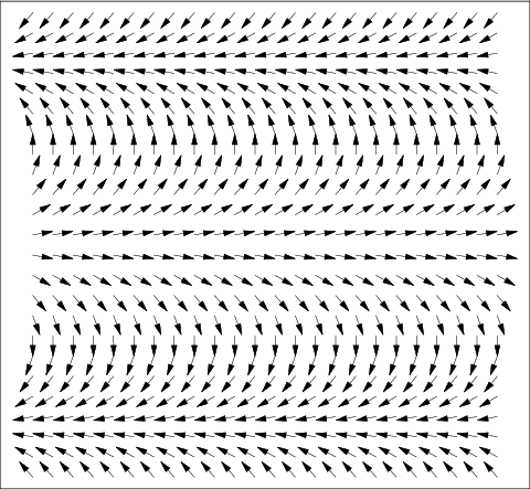
First, the energy of doped holes is calculated keeping the staggered magnetization field fixed. Then the parameters of the staggered magnetization field are varied in order to minimize the total energy.
III.1 Fermionic Contribution to the Energy
In this subsection we compute the fermionic contribution to the energy of a homogeneous or spiral configuration of the staggered magnetization. For the moment, we ignore the 4-fermion couplings. The considerations of this paper are valid only if the 4-fermion couplings are weak and can be treated in perturbation theory. Furthermore, we may neglect the vertices proportional to , , , and which involve two spatial derivatives and are thus of higher order than the hole-one-magnon vertex proportional to . The fermion Hamiltonian resulting from the leading terms of the Euclidean action is given by
| (16) | |||||
The covariant derivative takes the form
| (17) |
Here and are creation and annihilation operators (not Grassmann numbers) for fermions of flavor and spin (parallel or antiparallel to the local staggered magnetization), which obey canonical anticommutation relations. As before, and . The above Hamiltonian is invariant against time-independent gauge transformations
| (18) |
Here we consider holes propagating in the background of a configuration with
| (19) |
where and are real-valued constants. In other words, we focus on configurations of the staggered magnetization in which (after an appropriate gauge transformation) the fermions experience a constant composite vector field , which leads to a homogeneous fermion density. As was shown in [54], the most general configuration of this kind represents a spiral in the staggered magnetization. The Hamiltonian can then be diagonalized by going to momentum space. Since magnon exchange does not mix the flavors, the Hamiltonian can be considered separately for and , but it still mixes spin with . The single-particle Hamiltonian for holes with spatial momentum takes the form
| (20) |
The hole-one-magnon vertex proportional to mixes the spin and states and provides a potential mechanism to stabilize a spiral phase. The diagonalization of the above Hamiltonian yields
| (21) |
where . Interestingly, the above equation is independent of the flavor index . We will keep the flavor index to indicate that there are two flavors in our calculations. Since the energy depends only on , unlike in the square lattice case, potential spiral configurations do not prefer any particular spatial direction. This is due to the spatial rotation symmetry discussed in the previous section. However, one should keep in mind that is an accidental symmetry of just the leading terms in the effective action, which is broken explicitly by the higher-order terms. Hence, when the higher-order terms are included, one expects the spiral to align with a lattice direction. Mixing via the vertex lowers the energy and raises the energy . It should be noted that, in this case, the index no longer refers to the spin orientation. Indeed, the eigenvectors corresponding to are linear combinations of both spins. The minimum of the energy is located at for which
| (22) |
Since does not affect the magnon contribution to the energy density, we fix it by minimizing which implies . The energies of eq.(21) then reduce to
| (23) |
Consequently, the filled hole pockets are circles determined by
| (24) |
where is the kinetic energy of a hole in the pocket at the Fermi surface. The area of an occupied hole pocket determines the fermion density as
| (25) |
The kinetic energy density of a filled pocket is given by
| (26) |
The total density of fermions of all flavors is
| (27) | |||||
and the total energy density of the holes is
| (28) |
with
| (29) |
The filling of the various hole pockets is controlled by the parameters which must be varied in order to minimize the energy while keeping the total density of holes fixed. We thus introduce
| (30) |
where is a Lagrange multiplier that fixes the density, and we demand
| (31) |
III.2 Four Populated Hole Pockets
We will now populate the various hole pockets with fermions. First, we keep the configuration of the staggered magnetization fixed and we vary the in order to minimize the energy of the fermions. Then we also vary the parameters of the staggered magnetization field in order to minimize the total energy. One must distinguish various cases, depending on how many hole pockets are populated with fermions. In this subsection, we consider the case of populating all four hole pockets (i.e. with both flavors and with both energy indices ). In this case, eq.(31) implies
| (32) |
The total energy density then takes the form
| (33) | |||||
Here is the energy density of the system at half-filling. For the energy is minimized for and the configuration is thus homogeneous. The total energy density in the four-pocket case is then given by
| (34) |
For , on the other hand, the energy is not bounded from below. In this case, seems to grow without bound. However, according to eq.(32) this would lead to which is physically meaningless. What really happens is that two pockets get completely emptied and we are naturally led to the two-pocket case. Before turning to that case, for completeness we first discuss the three-pocket case.
III.3 Three Populated Hole Pockets
We now populate only three pockets with holes: the two pockets with the lower energies and as well as the pocket with the higher energy . Of course, alternatively one could also fill the -pocket. We now obtain
| (35) |
such that eq.(31) yields
| (36) |
The total energy density then takes the form
| (37) | |||||
For the energy density is bounded from below and its minimum is located at
| (38) |
The resulting energy density in the three-pocket case takes the form
| (39) |
It is energetically less favorable than the homogeneous phase because for . For one obtains which is unphysical. In fact, the -pocket is then completely emptied and we are again led to investigating the two-pocket case.
III.4 Two Populated Hole Pockets
We now populate only two pockets with holes. These are necessarily the pockets with the lower energies and . In this case we have
| (40) |
and thus eq.(31) now implies
| (41) |
The total energy density then takes the form
| (42) | |||||
The energy density is bounded from below and has its minimum at
| (43) |
The value at the minimum is given by
| (44) |
The two-pocket spiral phase is less stable than the homogeneous phase if , which is the case for . As we have seen, both the three- and the four-pocket calculation become meaningless for , because the kinetic energies then become negative which is unphysical. The two-pocket calculation, on the other hand, continues to make sense for .
III.5 One Populated Hole Pocket
Finally, let us populate only one hole pocket, say the states with energy . Of course, alternatively one could also occupy the -pocket. One now obtains
| (45) |
The total energy density then takes the form
| (46) | |||||
which is minimized for
| (47) |
and the corresponding energy density takes the form
| (48) |
The one-pocket spiral is always energetically less favorable than the two-pocket spiral.
IV Inclusion of 4-Fermion Couplings in Perturbation Theory
In this section the 4-fermion contact interactions are incorporated in perturbation theory. Depending on the microscopic system in question, the 4-fermion couplings may or may not be small. If they are large, the result of the perturbative calculation should not be trusted. In that case, one could still perform a variational calculation. In this work we limit ourselves to first order perturbation theory. We will distinguish four cases: the homogeneous phase, the three-pocket spiral, the two-pocket spiral, and the one-pocket spiral. Finally, depending on the values of the low-energy parameters, we determine which phase is energetically favorable.
IV.1 Four-Pocket Case
Let us first consider the homogeneous phase. The perturbation of the Hamiltonian due to the leading 4-fermion contact terms is given by
| (49) | |||||
It should be noted that and again are fermion creation and annihilation operators (and not Grassmann numbers). In the homogeneous phase the fermion density is equally distributed among the two spin orientations and the two flavors such that
| (50) |
The brackets denote expectation values in the unperturbed state. Since the fermions are uncorrelated, for or one has
| (51) |
Taking the 4-fermion contact terms into account in first order perturbation theory, the total energy density of eq.(34) receives an additional contribution and now reads
| (52) |
IV.2 Three-Pocket Case
For a spiral aligned along the -direction () with the eigenvectors of the single-particle Hamiltonian of eq.(20) corresponding to the energy eigenvalues are given by
| (53) |
Inserting this expression in eq.(49) allows us to evaluate the expectation value in the unperturbed states determined before. In the three-pocket case the states with energies , , as well as (or alternatively ), and with inside the respective hole pocket are occupied and one arrives at
| (54) |
As a result, the energy density of eq.(39) turns into
| (55) | |||||
IV.3 Two-Pocket Case
In this case only the states with energy and with inside the respective hole pocket are occupied and hence
| (56) |
As a result the energy density of eq.(44) turns into
| (57) |
IV.4 One-Pocket Case
In the one-pocket case only the states with energy (or alternatively with ) and with inside the corresponding hole pocket are occupied so that one has
| (58) |
In this case, the 4-fermion terms do not contribute to the energy density which thus maintains the form of eq.(48), i.e.
| (59) |
IV.5 Stability Ranges of Various Phases
Let us summarize the results of the previous subsections. The energy densities of the various phases take the form
| (60) |
According to eqs.(59), (57), (55), and (52), the compressibilities are given by
| (61) |
The compressibilities as functions of are shown in figure 6.

For large values of , spiral phases cost a large amount of magnetic energy and the homogeneous phase is more stable. To be more precise, in this regime one has . Notice that is always larger than for any value of . As decreases and reaches the value
| (62) |
at leading order in the 4-fermi couplings one finds . For smaller values of , the two-pocket spiral is energetically favored until becomes negative and the system becomes unstable against the formation of spatial inhomogeneities of a yet undetermined type.
It should be pointed out again that these results apply only if the 4-fermion contact interactions are weak. Even if the 4-fermion couplings are indeed small, the results presented in this work do not necessarily reveal the true nature of the ground state. Due to the variational nature of the calculation, one cannot exclude that the phases that we found may still be unstable in certain parameter regions. It is instructive to compare the results presented here with the results obtained in the square lattice case [54]. Qualitatively the stability ranges of various phases are the same for both lattice geometries except that the one-pocket spiral is never energetically favored on the honeycomb lattice while it is favorable in a small parameter regime on the square lattice.
V Conclusions and Outlook
In this paper we have used a systematic effective field theory for
antiferromagnetic magnons and holes on the honeycomb lattice to investigate the
dynamics of holes in the background of a staggered magnetization field. We
have limited ourselves to constant composite vector fields which
implies that the fermions experience a constant background field.
Interestingly, unlike in the square lattice case, due to the accidental
continuous spatial rotation symmetry, at leading order a spiral
does not have an a priori preferred spatial direction. However,
since the symmetry is broken explicitly by the higher-order
terms, once such terms are included, one expects the spiral to align with a
lattice direction. Finally, we investigated the stability of spiral phases in
the presence of 4-fermion couplings. Assuming that the 4-fermion couplings
can be treated perturbatively, we have seen that, for sufficiently large
values of , the homogeneous phase is energetically favored. With
decreasing , a two-pocket spiral becomes energetically more favorable.
On the other hand, in contrast to the square lattice case, the one-pocket
spiral is never favored. For small values of the two-pocket spiral
becomes unstable against the formation of inhomogeneities of a yet undetermined
type. In [63] the low-energy parameters , , and have
been determined in terms of the parameters and of the underlying
- model. It will be interesting to also determine the strength of the
hole-one-magnon vertex in order to decide which phase is realized in
this model. Further applications of the effective theory, including the
one-magnon exchange potential and the resulting two-hole bound states, are
currently under investigation.
Acknowledgments
We like to thank B. Bessire, M. Nyfeler, and M. Wirz for their collaboration on the construction of the effective action for magnons and holes on the honeycomb lattice. U.-J. W. likes to thank P. A. Lee for interesting discussions and the members of the Center for Theoretical Physics at MIT, where part of this work was performed, for their hospitality. C. P. H. would like to thank the members of the Institute for Theoretical Physics at Bern University for their hospitality. The work of C. P. H. is supported by CONACYT Grant No. 50744-F and by Grant Proyecto Cuerpo-Academico-56-UCOL. This work was also supported in part by funds provided by the Schweizerischer Nationalfonds (SNF). In particular, F. K. is supported by an SNF young researcher fellowship. The “Center for Research and Education in Fundamental Physics” at Bern University is supported by the “Innovations- und Kooperationsprojekt C-13” of the Schweizerische Universitätskonferenz (SUK/CRUS).
References
- [1] J. C. Bednorz and K. A. Müller, Z. Phys. B64 (1986) 189.
- [2] J. E. Hirsch, Phys. Rev. Lett. 54 (1985) 1317.
- [3] P. W. Anderson, Science 235 (1987) 1196.
- [4] C. Gros, R. Joynt, and T. M. Rice, Phys. Rev. B36 (1987) 381.
- [5] S. A. Trugman, Phys. Rev. B37 (1988) 1597.
- [6] B. I. Shraiman and E. D. Siggia, Phys. Rev. Lett. 60 (1988) 740; Phys. Rev. Lett. 61 (1988) 467; Phys. Rev. Lett. 62 (1989) 1564; Phys. Rev. B46 (1992) 8305.
- [7] J. R. Schrieffer, X. G. Wen, and S. C. Zhang, Phys. Rev. Lett. 60 (1988) 944; Phys. Rev. B39 (1989) 11663.
- [8] S. Chakravarty, B. I. Halperin, and D. R. Nelson, Phys. Rev. B39 (1989) 2344.
- [9] H. Neuberger and T. Ziman, Phys. Rev. B39 (1989) 2608.
- [10] C. L. Kane, P. A. Lee, and N. Read, Phys. Rev. B39 (1989) 6880.
- [11] X. G. Wen, Phys. Rev. B39 (1989) 7223.
- [12] D. S. Fisher, Phys. Rev. B39 (1989) 11783.
- [13] S. Sachdev, Phys. Rev. B39 (1989) 12232.
- [14] R. Shankar, Phys. Rev. Lett. 63 (1989) 203; Nucl. Phys. B330 (1990) 433.
- [15] P. W. Anderson, Phys. Rev. Lett. 64 (1990) 1839.
- [16] A. Singh and Z. Tešanović, Phys. Rev. B41 (1990) 614.
- [17] S. A. Trugman, Phys. Rev. B41 (1990) 892.
- [18] C. L. Kane, P. A. Lee, T. K. Ng, B. Chakraborty, and N. Read, Phys. Rev. B41 (1990) 2653.
- [19] V. Elser, D. A. Huse, B. I. Shraiman, and E. D. Siggia, Phys. Rev. B41 (1990) 6715.
- [20] E. Dagotto, R. Joynt, A. Moreo, S. Bacci, and E. Gagliano, Phys. Rev. B41 (1990) 9049.
- [21] B. Chakraborty, N. Read, C. Kane, and P. A. Lee, Phys. Rev. B42 (1990) 4819.
- [22] P. Hasenfratz and F. Niedermayer, Phys. Lett. B268 (1991) 231.
- [23] A. Auerbach and B. E. Larson, Phys. Rev. B43 (1991) 7800.
- [24] S. Sarker, C. Jayaprakash, H. R. Krishnamurthy, and W. Wenzel, Phys. Rev. B43 (1991) 8775.
- [25] R. Eder, Phys. Rev. B43 (1991) 10706.
- [26] E. Arrigoni and G. C. Strinati, Phys. Rev. B44 (1991) 7455.
- [27] J. Igarashi and P. Fulde, Phys. Rev. B45 (1992) 10419.
- [28] R. Frésard and P. Wölfle, J. Phys.: Condens. Matter 4 (1992) 3625.
- [29] P. Hasenfratz and F. Niedermayer, Z. Phys. B92 (1993) 91.
- [30] G. C. Psaltakis and N. Papanicolaou, Phys. Rev. B48 (1993) 456.
- [31] H. Mori and M. Hamada, Phys. Rev. B48 (1993) 6242.
- [32] O. P. Sushkov, Phys. Rev. B49 (1994) 1250.
- [33] A. V. Chubukov, T. Senthil, and S. Sachdev, Phys. Rev. Lett. 72 (1994) 2089; Nucl. Phys. B426 (1994) 601.
- [34] A. V. Chubukov and K. A. Musaelian, Phys. Rev. B51 (1995) 12605.
- [35] C. Zhou and H. J. Schulz, Phys. Rev. B52 (1995) R11557.
- [36] A. V. Chubukov and D. K. Morr, Phys. Rev. B57 (1998) 5298.
- [37] N. Karchev, Phys. Rev. B57 (1998) 10913.
- [38] L. O. Manuel and H. A. Ceccatto, Phys. Rev. B61 (2000) 3470.
- [39] M. Brunner, F. F. Assaad, and A. Muramatsu, Phys. Rev. B62 (2000) 15480.
- [40] O. P. Sushkov and V. N. Kotov, Phys. Rev. B70 (2004) 024503.
- [41] V. N. Kotov and O. P. Sushkov, Phys. Rev. B70 (2004) 195105.
- [42] S. Weinberg, Physica 96 A (1979) 327.
- [43] J. Gasser and H. Leutwyler, Nucl. Phys. B250 (1985) 465.
- [44] P. Hasenfratz and H. Leutwyler, Nucl. Phys. B343 (1990) 241.
- [45] H. Georgi, Weak Interactions and Modern Particle Theory, Benjamin-Cummings Publishing Company, 1984.
- [46] J. Gasser, M. E. Sainio, and A. Švarc, Nucl. Phys. B307 (1988) 779.
- [47] E. Jenkins and A. Manohar, Phys. Lett. B255 (1991) 558.
- [48] V. Bernard, N. Kaiser, J. Kambor, and U.-G. Meissner, Nucl. Phys. B388 (1992) 315.
- [49] T. Becher and H. Leutwyler, Eur. Phys. J. C9 (1999) 643.
- [50] F. Kämpfer, M. Moser, and U.-J. Wiese, Nucl. Phys. B729 (2005) 317.
- [51] C. Brügger, F. Kämpfer, M. Moser, M. Pepe, and U.-J. Wiese, Phys. Rev. B74 (2006) 224432.
- [52] C. Brügger, C. P. Hofmann, F. Kämpfer, M. Moser, M. Pepe, and U.-J. Wiese, Phys. Rev. B75 (2007) 214405.
- [53] C. Brügger, F. Kämpfer, M. Pepe, and U.-J. Wiese, Eur. Phys. J. B53 (2006) 433.
- [54] C. Brügger, C. P. Hofmann, F. Kämpfer, M. Pepe and U.-J. Wiese, Phys. Rev. B75 (2007) 014421.
- [55] K. Takada, H. Sakurai, E. Takayama-Muromachi, F. Izumi, R. Dilanian, and T. Sasaki, Nature (London) 422 (2003) 53.
- [56] G. Baskaran, Phys. Rev. Lett. 91 (2003) 097003.
- [57] A. E. Trumper, C. J. Gazza, and L. O. Manuel, Phys. Rev. B69 (2004) 184407.
- [58] D. P. Chen, H. C. Chen, A. Maljuk, A. Kulakov, H. Zhang, P. Lemmens, C. T. Lin, Phys. Rev. B70 (2004) 024506.
- [59] C. J. Milne, D. N. Argyriou, A. Chemseddine, N. Aliouane, J. Veira, S. Landsgesell, D. Alber, Phys. Rev. Lett. 93 (2004) 247007.
- [60] W. Zheng, J. Oitmaa, C. J. Hamer, and R. R. P. Singh, Phys. Rev. B70 (2004) 020504.
- [61] H. Watanabe and M. Ogata, J. Phys. Soc. Jpn. 74 (2005) 2901.
- [62] A. Lüscher, A. Läuchli, W. Zheng, and O. Sushkov, Phys. Rev. B73 (2006) 155118.
- [63] F. J. Jiang, F. Kämpfer, M. Nyfeler, and U.-J. Wiese, arXiv:0807.2977 [cond-mat.str-el].
- [64] E. V. Castro, N. M. R. Peres, K. S. D. Beach, and A. W. Sandvik, Phys. Rev. B73 (2006) 054422.
- [65] F. Kämpfer, F.-J. Jiang, B. Bessire, M. Wirz, C. P. Hofmann, and U.-J. Wiese, in preparation.