Probability density functions of work and heat near the stochastic resonance of a colloidal particle
Abstract
We study experimentally and theoretically the probability density functions of the injected and dissipated energy in a system of a colloidal particle trapped in a double well potential periodically modulated by an external perturbation. The work done by the external force and the dissipated energy are measured close to the stochastic resonance where the injected power is maximum. We show a good agreement between the probability density functions exactly computed from a Langevin dynamics and the measured ones. The probability density function of the work done on the particle satisfies the fluctuation theorem.
pacs
82.70.DdI Introduction
The study of fluctuations of the injected and dissipated power in a system driven out of equilibrium by an external force is nowadays a widely studied problem which is not yet completely understood. This is a very important and general issue within the context of Fluctuation Theorems (FT) which constitute extremely useful relations for characterizing the probabilities of observing entropy production or consumption in out of equilibrium systems. These relations were first observed in the simulations of a sheared fluid[7] and later proved both for chaotic dynamical systems [8] and for stochastic dynamics[9]. These works lead to different formulations which find powerful applications for measuring free-energy difference in biology (see e.g. [10] for a review). The hypothesis and the extensions of fluctuation theorems[11] have been tested in various experimental systems such as colloidal particles[13, 12, 27], mechanical oscillators[14], electric circuits[15] and optically driven single two-level systems[16]. The effect of anharmonic potential on the motion of a colloidal particle has been tested by Blickle et al [13, 17, 16]. In a recent experiment [26] it has been shown that FT holds for a colloidal particle confined in a double well potential and driven out of equilibrium near the stochastic resonance (see next section). The purpose of this article is to compare the probability density function (PDF) for work and heat measured in this experiment with those analytically computed from a non-linear Langevin dynamics. We also discuss the difference between the PDF obtained from a phase average of the driving and those obtained from a fixed phase only. Such a precise comparison between theory and experiment in a double well potential driven out of equilibrium has never been done before. There is only a numerical study, which has explored the distributions of the dissipated heat and of the work in a Langevin dynamics near the stochastic resonance [18, 19]. The paper is organized as follow. The properties of the stochastic resonance are recalled in the next section. The experimental set-up is described in section 3. The analytical PDF are derived in section 4. The comparison between the theoretical predictions and the experimental measurements is done in section 5. Finally we conclude in section 6.
II Stochastic resonance
A colloidal particle, confined in a double well potential, hops between the two wells at a rate , named the Kramers’ rate, which is determined by the height of the energy barrier between the two wells, specifically , where is a characteristic time, the Boltzmann constant and the heat bath temperature [1]. When the double well potential is modulated by an external periodic perturbation whose frequency is close to the system presents the stochastic resonance phenomenon[2], i.e. the hops of the particle between the two wells synchronize with the external forcing. The stochastic resonance has been widely studied in many different systems and it has been shown to be a bona fide resonance looking at the resident time[2, 3], the Fourier transform of the signal for different noise intensity[4]. Numerically, the stochastic resonance has been characterized by computing the injected work done by the external agent as a function of noise and frequency [5, 6]. In a recent experiment [26] some of us have studied experimentally the Steady State Fluctuation Theorem (SSFT) in a system composed by a Brownian particle trapped in a double well potential periodically modulated by an external driving force. We have measured the energy injected into the system by the sinusoidal perturbation and we have analyzed the distributions of work and heat fluctuations. We find that although the dynamics of the system is strongly non-linear the SSFT holds for the work integrated on time intervals which are only a few periods of the driving force. In this paper we will compare this measured PDF with those derived analytically from a Langevin dynamics in which the exact potential of the experiment has been used.
III Experimental Set-up
The experimental setup is composed by a custom built inverted
optical tweezers made of an oil-immersion objective (63,
N.A.=1.3) which focuses a laser beam (wavelength
nm) to the diffraction limit
for trapping glass beads (m in diameter). The silica beads are dispersed
in bidistilled water in very small concentration. The suspension is introduced
in the sample chamber of dimensions mm3,
then a single bead is trapped and moved away from others.
The position of the bead is tracked using a fast-camera with the
resolution of 108 nm/pixels which gives after treatment the
position of the bead with an accuracy better than 20 nm.
The trajectories of the bead are sampled at
50 Hz. The position of the trap can be easily displaced on the
focal plane of the objective by deflecting the laser beam using an
acousto-optic deflector (AOD). To construct the double well
potential the laser is focused alternatively at two different
positions at a rate of 5 kHz. The residence times (with
) of the laser in each of the two positions determine the
mean trapping strength felt by the trapped particle. Indeed if
the typical diffusion length of the bead
during this period is only 5 nm. As a consequence the bead feels
an average double-well potential:
| (1) |
where , and are determined by the laser intensity and by the distance of the two focal points. In our experiment the distance between the two spots is m, which produces a trap whose minima are at 0.45 m. The total intensity of the laser is mW on the focal plane which corresponds to an inter-well barrier energy . Starting from the static symmetric double-trap, () we modulate the depth of the wells at low frequency by modulating the residence times () during which the spot remains in each position. We keep the total intensity of the laser constant in order to produce a more stable potential. The modulation of the average intensity is harmonic at frequency and its amplitude , is of the average intensity in the static symmetric case. Thus the potential felt by the bead has the following profile in the axial direction:
| (2) |
with , , and . The amplitude of the time dependent perturbation is synchronously acquired with the bead trajectory. The parameters given here are average parameters since the coefficients , and ,obtained from fitted steady distributions at given phases, vary with the phase (, ).
An example of the measured potential at and at is shown on the Fig. 1a). The figure is obtained by measuring the two steady state probability distribution function of , (corresponding to and respectively) and by taking .

III.1 The equation of motion.
The position of the particle can be described by a Langevin equation:
| (3) |
with N s m-1 the friction coefficient and the stochastic force. The natural Kramers’ rate () for the particle is Hz at K. When the particle can experience a stochastic resonance when the forcing frequency is close to the Kramers’ rate. An example of the sinusoidal force with the corresponding position are shown on the figure 1b).
III.2 The work and the heat.
Since the synchronization is not perfect, sometimes the particle receives energy from the perturbation, sometimes the bead moves against the perturbation leading to a negative work on the system.
In the following, all energies are normalized by . From the trajectories, we compute the stochastic and the classical works done by the perturbation on the system and the heat exchanged with the bath. These three quantities are defined by the following equations as in ref.[20]:
| (4) | |||
where in this case is a multiple of the forcing period. We use both and because they give complementary information on the fluctuations of the energy injected by the external perturbation into the system (see ref. [24] and reference therein for a discussion on this point). For example, as discussed in ref.[26] is the total entropy production rate in this specific case [22]. The heat and the work, defined in eq.4, are related through the first principle of thermodynamics: , where , whereas the two works are related by a boundary term , where . Since the characteristic time evolution of the perturbation is small compared to the fluctuation of position and due to the harmonic form of the perturbation, the integrals are computed as follows:
| (5) | |||||
where is the sampling time. We checked that the direct computing of integrals of and gives the same results. It is important to stress that can either take any value (as it has been done in ref.[26]) or be a multiple of : the fluctuations in the two cases exhibit different PDFs, as we will see in the next sections. To compute the works and heat from experimental data for a given duration , we thus divide a single trajectory into different segments starting either with a fixed phase, or with different phases, before averaging the results over the whole trajectory, and then over different runs. In ref.[26] the average work received over one period has been measured for different frequencies ( in eq. 4). Each trajectory is here recorded during 3200 s in different consecutive runs, which corresponds to 160 up to 7500 forcing periods, for the range of frequencies explored. It has been found that the maximum injected energy is around the frequency Hz, which is comparable with half of the Kramers’ rate of the fixed potential Hz. This maximum of transferred energy shows that the stochastic resonance for a Brownian particle is a bona fide resonance, as it was previously shown in experiments using resident time distributions [3, 21] or directly in simulations [5, 6]. It is worth noting that the average values of work in the case of a periodic forcing do not dependent on their definitions: only the boundary terms, which vanish in average with time, are different [26]. As the difference between and has been discussed in ref.[26] we will focus here only on that, in order to simplify the notation, will be indicated by .
IV Equations for the W and Q PDFs
In this section we discuss the equation governing the time evolution of the work and heat PDFs. For a stochastic process described by eq. (3) the Fokker-Planck equation reads
| (6) |
where is the PDF associated to the coordinate , and . Here and in the following, the prime denotes derivative with respect to .
Let us consider the joint probability distribution function of the position and of the stochastic work : in ref. [29] it has been shown that the time evolution of such a function is governed by the partial differential equation
| (7) |
with the starting condition . The unconstrained probability distribution of the work is given by
| (8) |
By introducing the Fourier transform
| (9) |
eq. (7) becomes
| (10) |
with the starting condition . Note that, by using the Fourier transform definition eq. (9), the wavenumber associated to is a purely imaginary number, .
Let us now consider the joint probability distribution of the position and the heat exchanged by the brownian particle whose motion is described by eq. (3). The Fokker-Planck-like equation, governing the time evolution of such a function, reads [27, 28]
| (11) | |||||
with the starting condition . Note that we use here the opposite sign convention for , eq. (5), with respect to that adopted in ref. [27].
The unconstrained probability distribution functions of the heat reads
| (12) |
Let be the Fourier transform of , as given by
| (13) |
eq. (11) becomes
| (14) |
with the starting condition . In ref. [27], it has been shown that by introducing the function defined by
| (15) |
equation (14) simplifies, as one gets rid of the first order derivatives with respect to , and it becomes
| (16) |
with the starting condition as given by .
We now show that a similar simplification can be obtained for eq. (10): let be defined as
| (17) |
substituting into eq. (10), we obtain the following equation for :
| (18) |
The last equation is identical to (16), however its starting condition reads , which is different from the starting condition of eq. (16).
As is an imaginary number, one can split eq. (16) and eq. (18), in a set of two equations for the real and imaginary part. For example, eq. (18) becomes
| (19) | |||||
| (20) |
where and are the real and the imaginary part of , respectively.
Equations (19) and (20), and the analogous equations for and , can be solved numerically for any value of , and for any choice of the initial condition using, e.g., MATHEMATICA [30]. The functions and , can be thus obtained by using equations (17) and (15). The target functions and can then be obtained by taking the Fourier inverse transform, i.e. by inverting eqs. (9) and (13), respectively. Also in this case the computation can be performed numerically.
V Comparison with experiments
In this section, we compare the results for the work and heat PDFs, as obtained by solving the differential equations introduced in the previous section, with the experimental outcomes. We take the external driving frequency to be equal to Hz, to have a good statistic, by allowing the observation of the system over a sufficient number of periods. Such a value is close to the natural Kramers’ rate, which ensures that the system is in the stochastic resonance regime.
We first consider the distribution of the work over a single period of the external potential (2). The unconstrained probability distribution of the work , is obtained as follows. In order to solve eq. (10), we solve numerically eq. (6) up to the time , so as to ensure that the solution of eq. (6) represents the steady state distribution of the position of the particle. Such a solution is used as a starting condition for eq. (10), which is solved numerically up to time , i.e. along a single period, and for different values of , so as to obtain . The resulting unconstrained Fourier transform of the work PDF, defined as , is plotted in fig. 2 .
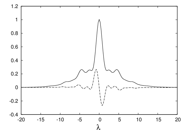
As discussed in the previous section, by inverting eq. (9) and exploiting eq. (8), we finally obtain . In fig. 3, the experimental histogram of the work done on the particle along a single period is plotted; in the same figure the unconstrained probability distribution of the work is also plotted. We find a good agreement between the experimental distribution of the work and the expected PDF. It is worth noting first that we start sampling only few periods after the beginning of each experiment and second that the experimental results are averaged over different values of in order to improve the statistics (either with a fixed phase or over different phases).

We now check that the work PDF satisfies the SSFT, which we expect to be true for any time which is an integer multiple of the period as discussed in [17, 23]. Given the periodicity of the external driving, the stochastic work here considered corresponds to the total entropy production, as defined by Seifert in [17, 23]. In figure 4, we plot the symmetry function for the work PDF, defined as
| (21) |
together with the corresponding work PDF, for two values of the final time . The fluctuation theorem states that the simmetry function has to satisfy the equality , for any value of . Inspection of the figure indicates that the fluctuation theorem is satisfied even at short times , the small deviations for the largest value of being due to numerical and experimental difficulties in the sampling of the tails of the work PDF. More details on SSFT have been already discussed in ref. [26].


We now consider the work distribution averaged over several phases. In order to obtain the probability distribution of the work, we solve eq. (6) up to the time , where and , i.e. we consider initial conditions with a phase difference . For each value of we solve eq. (10), up to time , so as to obtain , i.e. the Fourier transform of the work PDF with the starting condition , and by antitransforming, we obtain . Finally the average work PDF is obtained as . In fig. 5, this distribution is compared with the experimental outcomes. We find a good agreement between the expected PDF and the histogram of the work.

Similarly to what has been done for the work, we now consider the PDF of the heat , both with a single value of the initial phase, and averaged over several initial conditions. Also in this case, we use the function , solution of eq. (6), as a starting condition for the numerical integration of eq. (14), then by antitransforming the function , we obtain and finally , as discussed in the previous section. The results for the case of a single value of the initial phase is plotted in fig. 6, where we show a nice agreement with the experimental data.

In order to obtain the heat PDF averaged over several initial phases, we solve numerically eq. (14) in the time intervals , where , and have been defined above. Then by antitransforming the function , we obtain , and finally the unconstrained PDF of defined as . In fig. 7 we compare this expected PDF with the experimental outcomes, the agreement between the numerical PDF and the experimental data is good also in this case.

VI Conclusions
In conclusion, we have experimentally and theoretically investigated the power injected in a bistable colloidal system by an external oscillating force.
We have compared the PDFs of the stochastic work and of the heat measured in the experiment with those obtained theoretically. They exhibit large tails toward negative values and their shape are non-gaussian close to the resonance when averaging over a single period.
In refs. [27], it has been shown that if the external potential is quadratic, an analytical gaussian solution can be obtained for equation (7) at any value of and for eq. (11) in the long time limit. Here we have shown that the same equations can be solved numerically, also at finite time and for a more complex potentials, and they lead predictions on the system energy exchange that can be verified experimentally. We have shown that the Fourier transform of the heat and work PDFs obey the same differential equations (16) and (18), and the only difference lies in the initial conditions. This ensures and to be different at short time, while one has in the long time regime, as one would expect, since for long times.
Thus, our results suggest that the set of equations (7) and (11) represents an useful and general tool to investigate the energy balance of microscopic systems in arbitrary potentials.
Finally, we find that the work PDF satisfy the fluctuation theorem, even at short times.
Acknowledgements.
AI is grateful to L. Peliti for long and interesting discussions.References
- [1] A. Simon, A. Libchaber, Phys. Rev. Lett., 68, 3375 (1992).
- [2] R.Benzi,G. Parisi, A. Sutera,A. Vulpiani, SIAM J. Appl. Math., 43, 565 (1983).
- [3] L. Gammaitoni, F. Marchesoni and S. Santucci. Phys. Rev. Lett. 74 (7), 1052-1055 (1995).
- [4] D. Babic, C. Schmitt, I. Poberaj and C. Bechinger. Europhys. Lett. 67 (2), p. 158 (2004).
- [5] T. Iwai. Physica A 300, pp. 350-358 (2001)
- [6] D. Dan and A. M. Jayannavar. Physica A 345, pp. 404-410 (2005)
- [7] D. J. Evans, E. G. D. Cohen, and G. P. Morriss, Phys. Rev. Lett. 71, 2401 (1993); D. J. Evans and D. J. Searles, Phys. Rev. E 50, 1645 (1994).
- [8] G. Gallavotti, E. G. D. Cohen. Phys. Rev. Lett. 74, pp. 2694 - 2697 (1995).
- [9] Jorge Kurchan. J. Phys. A: Math. Gen. 31, pp. 3719?3729 (1998). J. L. Lebowitz and H. Spohn, J. Stat. Phys. 95, 333 (1999).
- [10] F. Ritort J. Phys.: Condens. Matter 18, R531 (2006).
- [11] R. van Zon and E.G.D. Cohen, Phys. Rev. Lett. 91 (11) 110601 (2003); Phys. Rev. E 67 046102 (2003); Phys. Rev. E 69 056121 (2004). R. van Zon, S. Ciliberto, E.G.D. Cohen, Phys. Rev. Lett. 92 (13) 130601 (2004).
- [12] G.M. Wang, E.M. Sevick, E. Mittag, D. J. Searles and D. J. Evans. Phys. Rev. Lett. 89, 050601 (2002)
- [13] V. Blickle, T. Speck, L. Helden, U. Seifert and C. Bechinger. Phys. Rev. Lett. 96, 070603 (2006).
- [14] F. Douarche, S. Joubaud, N. B. Garnier, A. Petrosyan, and S. Ciliberto Phys. Rev. Lett. 97 (14), 140603 (2006).
- [15] N. Garnier, S. Ciliberto, Phys. Rev. E 71 060101(R) (2005).
- [16] S. Schuler, T. Speck, C. Tietz, J. Wrachtrup and U. Seifert. Phys. Rev. Lett. 94, 180602 (2005).
- [17] T. Speck, V. Blickle, C. Bechinger and U. Seifert, Europhys.Lett, 79, 30002 (2007).
- [18] S. Saikia, R. Roy and A. M. Jayannavar. Phys. Lett. A, 369 pp. 367Ð371 (2007).
- [19] M. Sahoo, S. Saikia, M. C. Mahato and A. M. Jayannavar in press Physica A (2008).
- [20] K. Sekimoto J. Phys. Soc. Jpn. 66 (5), pp. 1234-1237 (1997).
- [21] C. Schmitt, B. Dybiec, P. Hänggi and C. Bechinger. Europhys. Lett. 74 (6), p. 937 (2006).
- [22] U. Seifert Eur. Phys. J. B, 64 3-4, pp. 423-431 (2008).
- [23] U. Seifert Phys. Rev. Lett. 95, 040602 (2005).
- [24] T. Taniguchi and E. G. D. Cohen J. Stat. Phys. 126 1 (2007)
- [25] T. Mai and A. Dhar. Phys. Rev. E 75, 061101 (2007)
- [26] P. Jop, A. Petrossyan, S. Ciliberto, Europhys. Lett., 81 50005 (2008).
- [27] A. Imparato, L. Peliti, G. Pesce, G. Rusciano, A. Sasso, Phys. Rev. E, 76 050101R (2007).
- [28] T. Speck and U. Seifert, J. Phys. A 38, L581 (2005).
- [29] A. Imparato and L. Peliti, Phys. Rev. E 72, 046114 (2005); A. Imparato and L. Peliti, Europhys. Lett. 70, 740 (2005).
- [30] S. Wolfram, The Mathematica Book (Cambridge University Press, Cambridge, 1999).