跳到论文正文
W Papers独立论文阅读器 arXiv:0809.4862 论文正文 计算阅读时间 · 0%
引用这篇论文根据当前论文元数据生成,正式投稿前建议核对。


License: arXiv.org perpetual non-exclusive license
arXiv:0809.4862v2 [math.DS] 29 Sep 2008

The cohomological equation for partially hyperbolic diffeomorphisms

Amie Wilkinson Address: Department of Mathematics, Northwestern University, 2033 Sheridan Rd., Evanston, IL 60208. USA
Date: August 24, 2026

Introduction

Let f:M→Mf:M\to M be a dynamical system and let ϕ:M→ℝ\phi\colon M\to{\mathbb{R}} be a function. Considerable energy has been devoted to describing the set of solutions to the cohomological equation:

(1) ϕ=Φ∘f−Φ,\displaystyle\phi=\Phi\circ f-\Phi,

under varying hypotheses on the dynamics of ff and the regularity of ϕ\phi. When a solution Φ:M→ℝ\Phi\colon M\to{\mathbb{R}} to this equation exists, then ϕ\phi is a called coboundary, for in the appropriate cohomology theory we have ϕ=d​Φ\phi=d\Phi. For historical reasons, a solution Φ\Phi to (1) is called a transfer function. The study of the cohomological equation has seen application in a variety of problems, among them: smoothness of invariant measures and conjugacies; mixing properties of suspended flows; rigidity of group actions; and geometric rigidity questions such as the isospectral problem. This paper studies solutions to the cohomological equation when ff is a partially hyperbolic diffeomorphism and ϕ\phi is CrC^{r}, for some real number r>0r>0.

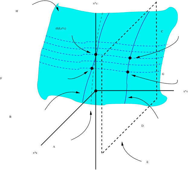
A a partially hyperbolic diffeomorphism f:M→Mf\colon M\to M of a compact manifold MM is one for which there exists a nontrivial, T​fTf-invariant splitting of the tangent bundle T​M=Es⊕Ec⊕EuTM=E^{s}\oplus E^{c}\oplus E^{u} and a Riemannian metric on MM such that vectors in EsE^{s} are uniformly contracted by T​fTf in this metric, vectors in EuE^{u} are uniformly expanded, and the expansion and contraction rates of vectors in EcE^{c} is dominated by the corresponding rates in EuE^{u} and EsE^{s}, respectively. An Anosov diffeomorphism is one for which the bundle EcE^{c} is trivial.

In the case where ff is an Anosov diffeomorphism, there is a wealth of classical results on this subject, going back to the seminal work of Livsic̆, which we summarize here in Theorem 0.1. Here and in the rest of the paper, the notation Ck,αC^{k,\alpha}, for k∈ℤ+k\in{\mathbb{Z}}_{+}, α∈(0,1]\alpha\in(0,1], means CkC^{k}, with α\alpha-Hölder continuous kkth derivative (where C0,αC^{0,\alpha}, α∈(0,1]\alpha\in(0,1] simply means α\alpha-Hölder continuous). For α∈(0,1)\alpha\in(0,1), CαC^{\alpha} means α\alpha-Hölder continuous. More generally, if r>0r>0 is not an integer, then we will also write CrC^{r} for C⌊r⌋,r−⌊r⌋C^{\lfloor r\rfloor,r-\lfloor r\rfloor}.

Theorem 0.1.

[L1, L2, LS, GK1, GK2, dlLMM, J, dlL1] Let f:M→Mf\colon M\to M be an Anosov diffeomorphism and let ϕ:M→ℝ\phi:M\to{\mathbb{R}} be Hölder continuous.

I. Existence of solutions. If ff is C1C^{1} and transitive, then (1) has a continuous solution Φ\Phi if and only if ∑x∈𝒪ϕ⁡(x)=0\sum_{x\in\mathcal{O}}\phi(x)=0, for every ff-periodic orbit 𝒪\mathcal{O}.

II. Hölder regularity of solutions. If ff is C1C^{1}, then every continuous solution to (1) is Hölder continuous.

III. Measurable rigidity. Let ff be C2C^{2} and volume-preserving. If there exists a measurable solution Φ\Phi to (1), then there is a continuous solution Ψ\Psi, with Ψ=Φ\Psi=\Phi a.e.

More generally, if ff is CrC^{r} and topologically transitive, for r>1r>1, and μ\mu is a Gibbs state for ff with Hölder potential, then the same result holds: if there exists a measurable function Φ\Phi such that (1) holds μ\mu-a.e., then there is a continuous solution Ψ\Psi, with Ψ=Φ\Psi=\Phi, μ\mu-a.e.

IV. Higher regularity of solutions. Suppose that r>1r>1 is not an integer, and suppose that ff and ϕ\phi are CrC^{r}. Then every continuous solution to (1) is CrC^{r}.

If ff and ϕ\phi are C1C^{1}, then every continuous solution to (1) is C1C^{1}.

If ff and ϕ\phi are real analytic, then every continuous solution to (1) is real analytic.

There are several serious obstacles to overcome in generalizing these results to partially hyperbolic systems. For one, while a transitive Anosov diffeomorphism has a dense set of periodic orbits, a transitive partially hyperbolic diffeomorphism might have no periodic orbits (for an example, one can take the time-tt map of a transitive Anosov flow, for an appropriate choice of tt). Hence the hypothesis appearing in part I can be empty: the vanishing of ∑x∈𝒪ϕ⁡(x)\sum_{x\in\mathcal{O}}\phi(x) for every periodic orbit of ff cannot be a complete invariant for solving (1).

This first obstacle was addressed by Katok and Kononenko [KK], who defined a new obstruction to solving equation (1) when ff is partially hyperbolic. To define this obstruction, we first define a relevant collection of paths in MM, called s​usu-paths, determined by a partially hyperbolic structure.

The stable and unstable bundles EsE^{s} and EuE^{u} of a partially hyperbolic diffeomorphism are tangent to foliations, which we denote by 𝒲s\mathcal{W}^{s} and 𝒲u\mathcal{W}^{u} respectively [BP]. The leaves of 𝒲s\mathcal{W}^{s} and 𝒲u\mathcal{W}^{u} are contractible, since they are increasing unions of submanifolds diffeomorphic to Euclidean space. An s​usu-path in MM is a concatenation of finitely many subpaths, each of which lies entirely in a single leaf of 𝒲s\mathcal{W}^{s} or a single leaf of 𝒲u\mathcal{W}^{u}. An s​usu-loop is an s​usu-path beginning and ending at the same point.

We say that a partially hyperbolic diffeomorphism f:M→Mf:M\to M is accessible if any point in MM can be reached from any other along an s​usu-path. The accessibility class of x∈Mx\in M is the set of all y∈My\in M that can be reached from xx along an s​usu-path. Accessibility means that there is one accessibility class, which contains all points. Accessibility is a key hypothesis in most of the results that follow. We remark that Anosov diffeomorphisms are easily seen to be accessible, by the transversality of EuE^{u} and EsE^{s} and the connectedness of MM.

Any finite tuple of points (x0,x1,…,xk)(x_{0},x_{1},\ldots,x_{k}) in MM with the property that xix_{i} and xi+1x_{i+1} lie in the same leaf of either 𝒲s\mathcal{W}^{s} or 𝒲u\mathcal{W}^{u}, for i=0,…,k−1i=0,\ldots,k-1, determines an s​usu-path from x0x_{0} to xkx_{k}; if in addition xk=x0x_{k}=x_{0}, then the sequence determines an s​usu-loop. Following [ASV], we call such a tuple (x0,x1,…,xk)(x_{0},x_{1},\ldots,x_{k}) an accessible sequence and if x0=xkx_{0}=x_{k}, an accessible cycle (the term periodic cycle is used in [KK]).

For ff a partially hyperbolic diffeomorphism, there is a naturally-defined periodic cycles functional

P​C​F:{accessible sequences}×Cα​(M)→ℝ.PCF\colon\{\hbox{accessible sequences}\}\times C^{\alpha}(M)\to{\mathbb{R}}.

which was introduced in [KK] as an obstruction to solving (1). For x∈Mx\in M and x′∈𝒲u​(x)x^{\prime}\in\mathcal{W}^{u}(x), we define:

P​C​F(x,x′)​ϕ=∑i=1∞ϕ⁡(f−i​(x))−ϕ⁡(f−i​(x′)),PCF_{(x,x^{\prime})}\phi=\sum_{i=1}^{\infty}\phi(f^{-i}(x))-\phi(f^{-i}(x^{\prime})),

and for x′∈𝒲s​(x)x^{\prime}\in\mathcal{W}^{s}(x), we define:

P​C​F(x,x′)​ϕ=∑i=0∞ϕ⁡(fi​(x′))−ϕ⁡(fi​(x)).PCF_{(x,x^{\prime})}\phi=\sum_{i=0}^{\infty}\phi(f^{i}(x^{\prime}))-\phi(f^{i}(x)).

The convergence of these series follows from the Hölder continuity of ϕ\phi and the expansion/contraction properties of the bundles EuE^{u} and EsE^{s}. This definition then extends to accessible sequences by setting P​C​F(x0,…,xk)​ϕ=∑i=0k−1P​C​F(xi,xi+1)​(ϕ)PCF_{(x_{0},\ldots,x_{k})}\phi=\sum_{i=0}^{k-1}PCF_{(x_{i},x_{i+1})}(\phi).

Assuming a hypothesis on ff called local accessibility11 1 A partially hyperbolic diffeomorphism f:M→Mf\colon M\to M is locally accessible if for every compact subset M1⊂MM_{1}\subset M there exists k≥1k\geq 1 such that for any ε>0\varepsilon>0, there exists δ>0\delta>0 that for every x,x′∈Mx,x^{\prime}\in M with x∈M1x\in M_{1} and d⁡(x,x′)<δd(x,x^{\prime})<\delta, there is an accessible sequence (x=x0,…,xk=x′)(x=x_{0},\ldots,x_{k}=x^{\prime}) from xx to x′x^{\prime} satisfying d⁡(xi,x)≤ε,andd𝒲∗​(xi+1,xi)<2​ε,fori=0,…,k−1d(x_{i},x)\leq\varepsilon,\quad\hbox{and}\quad d_{\mathcal{W}^{\ast}}(x_{i+1},x_{i})<2\varepsilon,\quad\hbox{for}\quad i=0,\ldots,k-1 where d𝒲∗d_{\mathcal{W}^{\ast}} denotes the distance along the 𝒲s\mathcal{W}^{s} or 𝒲u\mathcal{W}^{u} leaf common to the two points., [KK] proved that the closely related relative cohomological equation:

(2) ϕ=Φ∘f−Φ+c,\displaystyle\phi=\Phi\circ f-\Phi+c,

has a solution Φ:M→ℝ\Phi\colon M\to{\mathbb{R}} and c∈ℝc\in{\mathbb{R}}, with Φ\Phi continuous, if and only if P​C​Fγ​(ϕ)=0PCF_{\gamma}(\phi)=0, for every accessible cycle γ\gamma.

The local accessibility hypothesis in [KK] has been verified only for very special classes of partially hyperbolic systems, and it is not known whether there exist C1C^{1}-open sets of locally accessible diffeomorphisms, or more generally, whether accessibility implies local accessibility (although this seems unlikely). Assuming the strong hypothesis that EuE^{u} and EsE^{s} are C∞C^{\infty} bundles, [KK] also showed that a continuous transfer function for a C∞C^{\infty} coboundary is always C∞C^{\infty}.

In the first part of our main result, Theorem A, part I below, we show that the local accessibility hypothesis in [KK] can be replaced simply by accessibility. Accessibility is known to hold for a C1C^{1} open and dense subset of all partially hyperbolic systems [DW], is CrC^{r} open and dense among partially hyperbolic systems with 11-dimensional center [HHU, BHHTU], and is conjectured to hold for a CrC^{r} open and dense subset of all partially hyperbolic diffeomorphisms, for all r≥1r\geq 1 [PS]. Thus, part I of Theorem A gives a robust counterpart of part I of Theorem 0.1 for partially hyperbolic diffeomorphisms.

Another of the aforementioned major obstacles to generalizing Theorem 0.1 to the partially hyperbolic setting is that the regularity results in part IV fail to hold for general partially hyperbolic systems. Veech [V] and Dolgopyat [D] both exhibited examples of partially hyperbolic diffeomorphisms (volume-preserving and ergodic) where there is a sharp drop in regularity from ϕ\phi to a solution Φ\Phi. These examples are not accessible. Here we show in Theorem A, part IV, that assuming accessibility and a C1C^{1}-open property called strong rr-bunching (which incidentally is satisfied by the nonaccessible examples in [V, D]), there is no significant loss of regularity between ϕ\phi and Φ\Phi.

Part III of Theorem 0.1 is the most resistant to generalization, primarily because a general notion of Gibbs state for a partially hyperbolic diffeomorphism remains poorly understood. In the conservative setting, the most general result to date concerning ergodicity of for partially hyperbolic diffeomorphisms is due to Burns and Wilkinson [BW2], who show that every C2C^{2}, volume-preserving partially hyperbolic diffeomorphism that is center-bunched and accessible is ergodic. Center bunching is a C1C^{1}-open property that roughly requires that the action of T​fTf on EcE^{c} be close to conformal, relative to the expansion and contraction rates in EsE^{s} and EuE^{u} (see Section 2). Adopting the same hypotheses as in [BW2], we recover here the analogue of Theorem 0.1 part III for volume-preserving partially hyperbolic diffeomorphisms.

We now state our main result.

Theorem A.

Let f:M→Mf\colon M\to M be partially hyperbolic and accessible, and let ϕ:M→ℝ\phi:M\to{\mathbb{R}} be Hölder continuous.

I. Existence of solutions. If ff is C1C^{1}, then (2) has a continuous solution Φ\Phi for some c∈ℝc\in{\mathbb{R}} if and only if P​C​F𝒞​(ϕ)=0PCF_{\mathcal{C}}(\phi)=0, for every accessible cycle 𝒞\mathcal{C}.

II. Hölder regularity of solutions. If ff is C1C^{1}, then every continuous solution to (2) is Hölder continuous.

III. Measurable rigidity. Let ff be C2C^{2}, center bunched, and volume-preserving. If there exists a measurable solution Φ\Phi to (2), then there is a continuous solution Ψ\Psi, with Ψ=Φ\Psi=\Phi a.e.

IV. Higher regularity of solutions. Let k≥2k\geq 2 be an integer. Suppose that ff and ϕ\phi are both CkC^{k} and that ff is strongly rr-bunched, for some r<k−1r<k-1 or r=1r=1. If Φ\Phi is a continuous solution to (2), then Φ\Phi is CrC^{r}.

The center bunching and strong rr-bunching hypotheses in parts III and IV are C1C^{1}-open conditions and are defined in Section 2. Theorem A part IV generalizes all known C∞C^{\infty} Livšic regularity results for accessible partially hyperbolic diffeomorphisms. In particular, it applies to all time-tt maps of Anosov flows and compact group extensions of Anosov diffeomorphisms. Accessibility is a C1C^{1} open and C∞C^{\infty} dense condition in these classes [BW1, BPW]. In dimension 33, for example, the time-1 map of any mixing Anosov flow is stably accessible [BPW], unless the flow is a constant-time suspension of an Anosov diffeomorphism.

We also recover the results of [D] in the context of compact group extensions of volume-preserving Anosov diffeomorphisms. Finally, Theorem A also applies to all accessible, partially hyperbolic affine transformations of homogeneous manifolds. A direct corollary that encompasses these cases is:

Corollary 0.2.

Let ff be C∞C^{\infty}, partially hyperbolic and accessible. Assume that T​f|EcTf|_{E^{c}} is isometric in some continuous Riemannian metric. Let ϕ:M→ℝ\phi\colon M\to{\mathbb{R}} be C∞C^{\infty}. Suppose there exists a continuous function Φ:M→ℝ\Phi\colon M\to{\mathbb{R}} such that

ϕ=Φ∘f−Φ.\phi=\Phi\circ f-\Phi.

Then Φ\Phi is C∞C^{\infty}. If, in addition, ff preserves volume, then any measurable solution Φ\Phi extends to a C∞C^{\infty} solution.

For any such ff, and any integer k≥2k\geq 2, there is a C1C^{1} open neighborhood 𝒰\mathcal{U} of ff in Diffk​(M)\hbox{Diff}^{k}(M) such that, for any accessible g∈𝒰g\in\mathcal{U}, and any CkC^{k} function ϕ:M→ℝ\phi\colon M\to{\mathbb{R}}, if

ϕ=Φ∘g−Φ,\phi=\Phi\circ g-\Phi,

has a continuous solution Φ\Phi, then Φ\Phi is C1C^{1} and also CrC^{r}, for all r<k−1r<k-1. If gg also preserves volume, then any measurable solution extends to a CrC^{r} solution.

The vanishing of the periodic cycles obstruction in Theorem A, part I turns out to be a practical method in many contexts for determining whether (2) has a solution. On the one hand, this method has already been used by Damjanović and Katok to establish rigidity of certain partially hyperbolic abelian group actions [DK2]; in this (locally accessible, algebraic) context, checking that the P​C​FPCF obstruction vanishes reduces to questions in classical algebraic KK-theory (see also [DK1, NiţK]). On the other hand, for a given accessible partially hyperbolic system, the P​C​FPCF obstruction provides an infinite codimension obstruction to solving (2), and so the generic cocycle ϕ\phi has no solutions to (2). This latter fact follows from recent work of Avila, Santamaria and Viana on the related question of vanishing of Lyapunov exponents for linear cocycles over partially hyperbolic systems (see [ASV], section 9).

As part of proof of Theorem A, part II, we also prove that stable and unstable foliations of any C1C^{1} partially hyperbolic diffeomorphism are transversely Hölder continuous (Corollary 5.3). This extends to the C1C^{1} setting the well-known fact that the stable and unstable foliations for a C1+θC^{1+\theta} partially hyperbolic diffeomorphism are transversely Hölder continuous [PSW]. As far as we know, no previous regularity results were known for C1C^{1} systems, including Anosov diffeomorphisms.

In a forthcoming work [AVW] we will use some of the results here to prove rigidity theorems for partially hyperbolic diffeomorphisms and group actions.

We now summarize in more detail the previous results in this area:

  • •

    Veech [V] studied the case when ff is a partially hyperbolic toral automorphism and established existence and regularity results for solutions to (1). In these examples, there is a definite loss of regularity between coboundary and transfer function. The examples studied by Veech differ from those treated here in that they do not have the property of accessibility (although they have the weaker property of essential accessibility).

  • •

    Dolgopyat [D] studied equations (1) and (2) for a special class of partially hyperbolic diffeomorphisms – the compact group extensions of Anosov diffeomorphisms – in the case where the base map preserves a Gibbs state μ\mu with Hölder potential. Assuming rapid mixing of the group extension with respect to μ\mu, [D] showed that if the coboundary ϕ\phi is C∞C^{\infty}, then any transfer function Φ∈L2​(μ×Haar)\Phi\in L^{2}(\mu\times{\hbox{Haar}}) is also C∞C^{\infty}. Dolgopyat also gave an example of a partially hyperbolic diffeomorphism with a C∞C^{\infty} coboundary whose transfer map is continuous, but not C1C^{1}. This example, like Veech’s, is essentially accessible, but not accessible. We note that when the Gibbs measure μ\mu is volume, then the rapid mixing assumption in [D] is equivalent to accessibility.

  • •

    De la Llave [dlL2], extended the work of [KK] to give some regularity results for the transfer function under strong (nongeneric) local accessibility/regularity hypotheses on bundles. De la Llave’s approach focuses on bootstrapping the regularity of the transfer function from LpL^{p} to continuity and higher smoothness classes using the transverse regularity of the stable and unstable foliations in MM. For this reason, he makes strong regularity hypotheses on this transverse regularity.

While there are superficial similaries between these previous results and Theorem A, the approach here, especially in parts II and IV, is fundamentally new and does not rely on these results. In particular, to establish regularity of a transfer function, we take advantage of a form of self-similarity of its graph in the central directions of MM. This self-similarity, known as CrC^{r} homogeneity is discussed in more detail in the following section.

1. Techniques in the proof of Theorem A

The proof of parts I and III of Theorem A use recent work of Avila, Santamaria and Viana on sections of bundles with various saturation properties. In [ASV], they apply these results to show that under suitable conditions, matrix cocycles over partially hyperbolic systems have a nonvanishing Lyapunov exponent. Parts I and III of Theorem A are translations of some of the main results in [ASV] to the abelian cocycle setting.

The regularity results in Theorem A – parts II and IV – comprise the bulk of this paper.

To investigate the regularity of a solution Φ\Phi, we examine the graph of Φ\Phi in M×ℝM\times{\mathbb{R}}. If ϕ\phi is Hölder continuous, then the stable and unstable foliations 𝒲s\mathcal{W}^{s} and 𝒲u\mathcal{W}^{u} for ff lift to two “stable and unstable” foliations 𝒲ϕs\mathcal{W}^{s}_{\phi} and 𝒲ϕu\mathcal{W}^{u}_{\phi} of M×ℝM\times{\mathbb{R}}, whose leaves are graphs of Hölder continuous functions into ℝ{\mathbb{R}}. These lifted foliations are invariant under the skew product (x,t)↦(f⁡(x),t+ϕ⁡(x))(x,t)\mapsto(f(x),t+\phi(x)). The fact that Φ\Phi satisfies the equation ϕ=Φ∘f−Φ+c\phi=\Phi\circ f-\Phi+c, for some c∈ℝc\in{\mathbb{R}}, implies that the graph of Φ\Phi is saturated by leaves of the lifted foliations. The leafwise and transverse regularity of these foliations determine the regularity of Φ\Phi. In the most general setting of Theorem A, part II, these foliations are both leafwise and transversely Hölder continuous, and this implies the Hölder regularity of Φ\Phi when ff is accessible.

The proof of higher regularity in part IV has two main components. We first describe a simplified version of the proof under an additional assumption on ff called dynamical coherence.

Definition 1.1.

A partially hyperbolic diffeomorphism ff is dynamically coherent if the distributions Ec⊕EuE^{c}\oplus E^{u}, and Ec⊕EsE^{c}\oplus E^{s} are integrable, and everywhere tangent to foliations 𝒲c​u\mathcal{W}^{cu} and 𝒲c​s\mathcal{W}^{cs}.

If ff is dynamically coherent, then there is also a central foliation 𝒲c\mathcal{W}^{c}, tangent to EcE^{c}, whose leaves are obtained by intersecting the leaves of 𝒲c​u\mathcal{W}^{cu} and 𝒲c​s\mathcal{W}^{cs}. The normally hyperbolic theory [HPS] implies that the leaves of 𝒲c​u\mathcal{W}^{cu} are then bifoliated by the leaves of 𝒲c\mathcal{W}^{c} and 𝒲u\mathcal{W}^{u}, and the leaves of 𝒲c​s\mathcal{W}^{cs} are bifoliated by the leaves of 𝒲c\mathcal{W}^{c} and 𝒲s\mathcal{W}^{s}.

Suppose that ff is dynamically coherent and that ff and ϕ\phi satisfy the hypotheses of part IV of Theorem A, for some k≥2k\geq 2 and r<k−1r<k-1 or r=1r=1. Under these assumptions, here are the two components of the proof. The first part of the proof is to show that Φ\Phi is uniformly CrC^{r} along individual leaves of 𝒲s\mathcal{W}^{s}, 𝒲u\mathcal{W}^{u} and 𝒲c\mathcal{W}^{c}. The second part is to employ a result of Journé to show that smoothness of Φ\Phi along leaves of these three foliations implies smoothness of Φ\Phi.

To show that Φ\Phi is smooth along the leaves of 𝒲s\mathcal{W}^{s} and 𝒲u\mathcal{W}^{u}, we examine again the lifted foliations for the associated skew product. The assumption that ϕ\phi is CkC^{k} implies that the leaves of these lifted foliations are CrC^{r} (in fact, they are CkC^{k}). This part of the proof does not require dynamical coherence or accessibility.

To show that Φ\Phi is smooth along leaves of the central foliation, one can use accessibility and strong rr-bunching to show that the graph of Φ\Phi over any central leaf 𝒲c​(x)\mathcal{W}^{c}(x) of ff is CrC^{r} homogeneous. More precisely, setting N′=𝒲c​(x)×ℝN^{\prime}=\mathcal{W}^{c}(x)\times{\mathbb{R}} and N={(y,Φ⁡(y)):y∈𝒲c​(x)}⊂N′N=\{(y,\Phi(y)):y\in\mathcal{W}^{c}(x)\}\subset N^{\prime}, we show that the manifold NN is CrC^{r} homogeneous in N′N^{\prime}: for any two points p,q∈Np,q\in N, there is a CrC^{r} local diffeomorphism of N′N^{\prime} sending pp to qq and preserving NN. C1C^{1}-homogeneous subsets of a manifold have a remarkable property:

Theorem 1.2.

[RSS] Any locally compact subset NN of a C1C^{1} manifold N′N^{\prime} that is C1C^{1} homogeneous in N′N^{\prime} is a C1C^{1} submanifold of N′N^{\prime}

If r=1r=1, we can apply this result to obtain that the graph of Φ\Phi is C1C^{1} over any center manifold. Hence Φ\Phi is C1C^{1} over center, stable, and unstable leaves, which implies that Φ\Phi is C1C^{1}. This completes the proof in the case r=1r=1 (assuming dynamical coherence).

In fact we do not use the results in [RSS] in the proof of Theorem A but employ a different technique to establish smoothness, which also works for r>1r>1 and in the non-dynamically coherent case. Our methods also show:

Theorem B.

For any integer k≥2k\geq 2, any CkC^{k} homogeneous, C1C^{1} submanifold of a CkC^{k} manifold is a CkC^{k} submanifold.

Theorem B is stated in [RSS] without proof. In a recent article [S] by the third author of [RSS], the problem of whether a CkC^{k} homogeneous submanifold a CkC^{k} submanifold is stated as open for k>1k>1 (and conjectured to hold). Combining Theorems 1.2 and  B, we obtain a proof of the conjecture in [S]:

Corollary 1.3.

Let k≥1k\geq 1 be an integer. Then any locally compact subset of a CkC^{k} manifold that is CkC^{k} homogeneous is a CkC^{k} submanifold.

A proof of Theorem B is given in [BM] under the assumption that the submanifold is CkC^{k} homogeneous under the continuous action of a Lie group by diffeomorphisms. It appears that Theorem B is not an obvious consequence of Theorem 1.2 (see the remark after the proof of Lemma 7.1).

Returning to the proof of Theorem A, assuming dynamical coherence and using Corollary 1.3, one can obtain under the hypotheses of part IV that the graph of the transfer function Φ\Phi over each center manifold is C⌊r⌋C^{\lfloor r\rfloor}. With some more work, one can obtain that the graph of the transfer function Φ\Phi over each center manifold is CrC^{r}. A result of Journé [J] implies that for any r>1r>1 that is not an integer, and any two transverse foliations with uniformly CrC^{r} leaves, if a function Φ\Phi is uniformly CrC^{r} along the leaves of both foliations, then it is uniformly CrC^{r}. Since ff is assumed to be dynamically coherent, the 𝒲c\mathcal{W}^{c} and 𝒲s\mathcal{W}^{s} foliations transversely subfoliate the leaves of 𝒲c​s\mathcal{W}^{cs} . Applying Journé’s result using 𝒲c\mathcal{W}^{c} and 𝒲s\mathcal{W}^{s}, we obtain that Φ\Phi is CrC^{r} along the leaves of 𝒲c​s\mathcal{W}^{cs}. Applying Journé’s theorem again, this time with 𝒲c​s\mathcal{W}^{cs} and 𝒲u\mathcal{W}^{u}, we obtain that Φ\Phi is CrC^{r}.

We have just described a proof of part IV under the assumption that ff is dynamically coherent. If we drop the assumption of dynamical coherence, the assertion that Φ\Phi is “CrC^{r} along center manifolds” no longer makes sense, as ff might not have center manifolds. One can find locally invariant center manifolds that are “nearly” tangent to the center distribution (as in [BW2]), but the argument described above does not work for these manifolds. The analysis becomes considerably more delicate and is described in more detail in Section 8. As one of the components in our argument, we prove a strengthened version of Journé’s theorem (Theorem 8.4) that works for plaque families as well as foliations, and replaces the assumption of smoothness along leaves with the existence of an “approximate rr-jet” at the basepoint of each plaque.

The main result that lies behind the proof of Theorem A, part IV is a saturated section theorem for fibered partially hyperbolic systems (Theorem C). A fibered partially hyperbolic diffeomorphism is defined on a fiber bundle and is also a bundle isomorphism, covering a partially hyperbolic diffeomorphism (see Section 9). In this context, Theorem C states that under the additional hypotheses that the bundle diffeomorphism is suitably bunched, and the base diffeomorphism is accessible, then any continuous section of the bundle whose image is an accessibility class for the lifted map is in fact a smooth section. Using Theorem C it is also possible to extend in part the conclusions of Theorem A part IV to (suitably bunched) cocycles taking values in other Lie groups. The details are not carried out here, but the reader is referred to [NiţT, BW1, AV], where some of the relevant technical considerations are addressed (see also the remark after the statement of Theorem C in Section 9).

Theorem C would follow immediately if the following conjecture is correct.

Conjecture 1.4.

Let f:M→Mf\colon M\to M be CrC^{r}, partially hyperbolic and rr-bunched. Then every accessibility class for ff is an injectively immersed, CrC^{r} submanifold of MM.

For locally compact accessibility classes, it should be possible to prove Conjecture 1.4 using the techniques from [RSS] to show that the accessiblity class is a submanifold and the methods developed in this paper to show that the submanifold is smooth.

2. Partial hyperbolicity and bunching conditions

We now define the bunching hypotheses in Theorem A; to do so, we give a more precise definition of partial hyperbolicity. Let f:M→Mf:M\to M be a diffeomorphism of a compact manifold MM. We say that ff is partially hyperbolic if the following holds. First, there is a nontrivial splitting of the tangent bundle, T​M=Es⊕Ec⊕EuTM=E^{s}\oplus E^{c}\oplus E^{u}, that is invariant under the derivative map T​fTf. Further, there is a Riemannian metric for which we can choose continuous positive functions ν\nu, ν^\hat{\nu}, γ\gamma and γ^\hat{\gamma} with

(3) ν,ν^<1 and ν<γ<γ^−1<ν^−1\displaystyle\nu,\hat{\nu}<1\quad\hbox{ and }\quad\nu<\gamma<\hat{\gamma}^{-1}<\hat{\nu}^{-1}

such that, for any unit vector v∈Tp​Mv\in T_{p}M,

(4) ∥\displaystyle\| T​f​v|<ν⁡(p),\displaystyle Tfv\|<\nu(p), if ​v∈Es​(p),\displaystyle\qquad\hbox{if }v\in E^{s}(p),
(5) γ(p)<∥\displaystyle\gamma(p)<\| T​f​v|<γ^​(p)−1,\displaystyle Tfv\|<\hat{\gamma}(p)^{-1}, if ​v∈Ec​(p),\displaystyle\qquad\hbox{if }v\in E^{c}(p),
(6) ν^(p)−1<∥\displaystyle\hat{\nu}(p)^{-1}<\| Tfv∥,\displaystyle Tfv\|, if ​v∈Eu​(p).\displaystyle\qquad\hbox{if }v\in E^{u}(p).

We say that ff is center bunched if the functions ν,ν^,γ\nu,\hat{\nu},\gamma, and γ^\hat{\gamma} can be chosen so that:

(7) max⁡{ν,ν^}<γ​γ^.\displaystyle\max\{\nu,\hat{\nu}\}<\gamma\hat{\gamma}.

Center bunching means that the hyperbolicity of ff dominates the nonconformality of T​fTf on the center. Inequality (7) always holds when T​f|EcTf|_{E^{c}} is conformal. For then we have ‖Tp​f​v‖=‖Tp​f|Ec​(p)‖\|T_{p}fv\|=\|T_{p}f|_{E^{c}(p)}\| for any unit vector v∈Ec​(p)v\in E^{c}(p), and hence we can choose γ⁡(p)\gamma(p) slightly smaller and γ^​(p)−1\hat{\gamma}(p)^{-1} slightly bigger than

‖Tp​f|Ec​(p)‖.\|T_{p}f|_{E^{c}(p)}\|.

By doing this we may make the ratio γ⁡(p)/γ^​(p)−1=γ⁡(p)​γ^​(p)\gamma(p)/\hat{\gamma}(p)^{-1}=\gamma(p)\hat{\gamma}(p) arbitrarily close to 1, and hence larger than both ν⁡(p)\nu(p) and ν^​(p)\hat{\nu}(p). In particular, center bunching holds whenever EcE^{c} is one-dimensional. The center bunching hypothesis considered here is natural and appears in other contexts, e.g. [BP, BV, AV, NiţT, NicP].

For r>0r>0, we say that ff is rr-bunched if the functions ν,ν^,γ\nu,\hat{\nu},\gamma, and γ^\hat{\gamma} can be chosen so that:

(8) ν<γr,ν^<γ^r\displaystyle\nu<\gamma^{r},\qquad\hat{\nu}<\hat{\gamma}^{r}
(9) ν<γ​γ^r,and ν^<γ^​γr.\displaystyle\nu<\gamma\hat{\gamma}^{r},\quad\hbox{and }\quad\hat{\nu}<\hat{\gamma}\gamma^{r}.

Note that every partially hyperbolic diffeomorphism is rr-bunched, for some r>0r>0. The condition of 00-bunching is merely a restatement of partial hyperbolicity, and 11-bunching is center bunching. The first pair of inequalities in (8) are rr-normal hyperbolicity conditions; when ff is dynamically coherent, these inequalities ensure that the leaves of 𝒲c​u\mathcal{W}^{cu}, 𝒲c​s\mathcal{W}^{cs}, and 𝒲c\mathcal{W}^{c} are CrC^{r}. Combined with the first group of inequalities, the second group of inequalities imply that EuE^{u} and EsE^{s} are “CrC^{r} in the direction of EcE^{c}.” More precisely, in the case that ff is dynamically coherent, the rr-bunching inqualities imply that the restriction of EuE^{u} to 𝒲c​u\mathcal{W}^{cu} leaves is a CrC^{r} bundle and the restriction of EsE^{s} to 𝒲c​s\mathcal{W}^{cs} leaves is a CrC^{r} bundle.

For r>0r>0, we say that ff is strongly rr-bunched if the functions ν,ν^,γ\nu,\hat{\nu},\gamma, and γ^\hat{\gamma} can be chosen so that:

(10) max⁡{ν,ν^}<γr,max⁡{ν,ν^}<γ^r\displaystyle\max\{\nu,\hat{\nu}\}<\gamma^{r},\qquad\max\{\nu,\hat{\nu}\}<\hat{\gamma}^{r}
(11) ν<γ​γ^r,and ν^<γ^​γr.\displaystyle\nu<\gamma\hat{\gamma}^{r},\quad\hbox{and }\quad\hat{\nu}<\hat{\gamma}\gamma^{r}.

We remark that if ff is partially hyperbolic and there exists a Riemannian metric in which T​f|EcTf|_{E^{c}} is isometric, then ff is strongly rr-bunched, for every r>0r>0; given a metric ∥⋅∥\|\cdot\| for which ff satisfies (4), and another metric ∥⋅∥′\|\cdot\|^{\prime} in which T​f|EcTf|_{E^{c}} is isometric, it is a straighforward exercise to construct a Riemannian metric ∥⋅∥′′\|\cdot\|^{\prime\prime} for which inequalities (10) hold, with γ=γ^≡1\gamma=\hat{\gamma}\equiv 1.

The reason strong rr-bunching appears as a hypothesis in Theorem A is the following. Suppose that ff is partially hyperbolic and that ϕ:M→ℝ\phi\colon M\to{\mathbb{R}} is C1C^{1}. Then the skew product fϕ:M×ℝ/ℤ→M×ℝ/ℤf_{\phi}\colon M\times{\mathbb{R}}/{\mathbb{Z}}\to M\times{\mathbb{R}}/{\mathbb{Z}} given by

fϕ​(x,t)=(f⁡(x),t+ϕ⁡(x))f_{\phi}(x,t)=(f(x),t+\phi(x))

is partially hyperbolic, and if ff is strongly rr-bunched then fϕf_{\phi} is rr-bunched. This skew product and the corresponding lifted skew product on M×ℝM\times{\mathbb{R}} appears in a central way in our analysis, as we explain in the following section.

2.1. Notation

Let aa and bb be real-valued functions, with b≠0b\neq 0. The notation a=O⁡(b)a=O(b) means that the ratio |a/b||a/b| is bounded above, and a=Ω⁡(b)a=\Omega(b) means |a/b||a/b| is bounded below; a=Θ⁡(b)a=\Theta(b) means that |a/b||a/b| is bounded above and below. Finally, a=o⁡(b)a=o(b) means that |a/b|→0|a/b|\to 0 as b→0b\to 0. Usually aa and bb will depend on either an integer jj or a real number tt and on one or more points in MM. The constant CC bounding the appropriate ratios must be independent of nn or tt and the choice of the points.

The notation α<β\alpha<\beta, where α\alpha and β\beta are continuous functions, means that the inequality holds pointwise, and the function min⁡{α,β}\min\{\alpha,\beta\} takes the value min⁡{α⁡(p),β⁡(p)}\min\{\alpha(p),\beta(p)\} at the point pp.

We denote the Euclidean norm by |⋅||\cdot|. If XX is a metric space and r>0r>0 and x∈Xx\in X, the notation BX​(x,r)B_{X}(x,r) denotes the open ball about xx of radius rr. If the subscript is omitted, then the ball is understood to be in MM. Throughout the paper, rr always denotes a real number and j,k,ℓ,m,nj,k,\ell,m,n always denote integers. II denotes the interval (−1,1)⊂ℝ(-1,1)\subset{\mathbb{R}}, and In⊂ℝnI^{n}\subset{\mathbb{R}}^{n} the nn-fold product.

If γ1\gamma_{1} and γ2\gamma_{2} are paths in MM, then γ1⋅γ2\gamma_{1}\cdot\gamma_{2} denotes the concatenated path, and γ¯1\overline{\gamma}_{1} denotes the reverse path.

Suppose that ℱ\mathcal{F} is a foliation of an mm-manifold MM with dd-dimensional smooth leaves. For r>0r>0, we denote by ℱ⁡(x,r)\mathcal{F}(x,r) the connected component of xx in the intersection of ℱ⁡(x)\mathcal{F}(x) with the ball B⁡(x,r)B(x,r).

A foliation box for ℱ\mathcal{F} is the image UU of ℝm−d×ℝd{\mathbb{R}}^{m-d}\times{\mathbb{R}}^{d} under a homeomorphism that sends each vertical ℝd{\mathbb{R}}^{d}-slice into a leaf of ℱ\mathcal{F}. The images of the vertical ℝd{\mathbb{R}}^{d}-slices will be called local leaves of ℱ\mathcal{F} in UU.

A smooth transversal to ℱ\mathcal{F} in UU is a smooth codimension-dd disk in UU that intersects each local leaf in UU exactly once and whose tangent bundle is uniformly transverse to T​ℱT\mathcal{F}. If Σ1\Sigma_{1} and Σ2\Sigma_{2} are two smooth transversals to ℱ\mathcal{F} in UU, we have the holonomy map hℱ:Σ1→Σ2h_{\mathcal{F}}:\Sigma_{1}\to\Sigma_{2}, which takes a point in Σ1\Sigma_{1} to the intersection of its local leaf in UU with Σ2\Sigma_{2}.

Finally, for r>1r>1 a nonintegral real number, M,NM,N smooth manifolds, the CrC^{r} metric on Cr​(M,N)C^{r}(M,N) is defined in local charts by:

dCr​(f,g)=dC⌊r⌋​(f,g)+dC0​(D⌊r⌋​f,D⌊r⌋​g).d_{C^{r}}(f,g)=d_{C^{\lfloor r\rfloor}}(f,g)+d_{C^{0}}(D^{\lfloor r\rfloor}f,D^{\lfloor r\rfloor}g).

This metric generates the (weak) CrC^{r} topology on Cr​(M,N)C^{r}(M,N).

3. The partially hyperbolic skew product associated to a cocycle

Let f:M→Mf:M\to M be CkC^{k} and partially hyperbolic and let ϕ:M→ℝ\phi:M\to{\mathbb{R}} be Cℓ,αC^{\ell,\alpha}, for some integer ℓ≥0\ell\geq 0 and α∈[0,1]\alpha\in[0,1], with 0<ℓ+α≤k0<\ell+\alpha\leq k. Define the skew product fϕ:M×ℝ→M×ℝf_{\phi}:M\times{\mathbb{R}}\to M\times{\mathbb{R}} by

fϕ​(p,t)=(f⁡(p),t+ϕ⁡(p)).f_{\phi}(p,t)=(f(p),t+\phi(p)).

The following proposition is the starting point for our proof of Theorem A.

Proposition 3.1.

There exist foliations 𝒲ϕu,𝒲ϕs\mathcal{W}^{u}_{\phi},\mathcal{W}^{s}_{\phi} of M×ℝM\times{\mathbb{R}} with the following properties.

  1. (1)

    The leaves of 𝒲ϕu,𝒲ϕs\mathcal{W}^{u}_{\phi},\mathcal{W}^{s}_{\phi} are Cℓ,αC^{\ell,\alpha}.

  2. (2)

    The leaves of 𝒲ϕu\mathcal{W}^{u}_{\phi} project to leaves of 𝒲u\mathcal{W}^{u}, and the leaves of 𝒲ϕs\mathcal{W}^{s}_{\phi} project to leaves of 𝒲s\mathcal{W}^{s}. Moreover, (x′,t′)∈𝒲ϕs​(x,t)(x^{\prime},t^{\prime})\in\mathcal{W}^{s}_{\phi}(x,t) if and only if x′∈𝒲s​(x)x^{\prime}\in\mathcal{W}^{s}(x) and

    lim infn→∞d⁡(fϕn​(x,t),fϕn​(x′,t′))=0.\liminf_{n\to\infty}d(f_{\phi}^{n}(x,t),f_{\phi}^{n}(x^{\prime},t^{\prime}))=0.
  3. (3)

    Define T:ℝ×M→ℝ×MT\colon{\mathbb{R}}\times M\to{\mathbb{R}}\times M by Tt​(z,s)=(z,s+t)T_{t}(z,s)=(z,s+t). Then for all z∈Mz\in M and s,t∈ℝs,t\in{\mathbb{R}}:

    𝒲ϕs​(z,s+t)=Tt​𝒲ϕs​(z,s).\mathcal{W}^{s}_{\phi}(z,s+t)=T_{t}\mathcal{W}^{s}_{\phi}(z,s).
  4. (4)

    If (x,t)∈M×ℝ(x,t)\in M\times{\mathbb{R}} and (x′,t′)∈𝒲ϕs​(x,t)(x^{\prime},t^{\prime})\in\mathcal{W}^{s}_{\phi}(x,t), then

    t′−t=∑i=0∞ϕ⁡(fi​(x′))−ϕ⁡(fi​(x))=P​C​F(x,x′)​ϕ,t^{\prime}-t=\sum_{i=0}^{\infty}\phi(f^{i}(x^{\prime}))-\phi(f^{i}(x))=PCF_{(x,x^{\prime})}\phi,

    and if (x′,t′)∈𝒲ϕu​(x,t)(x^{\prime},t^{\prime})\in\mathcal{W}^{u}_{\phi}(x,t), then

    t′−t=∑i=1∞ϕ⁡(f−i​(x))−ϕ⁡(f−i​(x′))=P​C​F(x,x′)​ϕ.t^{\prime}-t=\sum_{i=1}^{\infty}\phi(f^{-i}(x))-\phi(f^{-i}(x^{\prime}))=PCF_{(x,x^{\prime})}\phi.
Proof.

The map fϕf_{\phi} covers the map (x,t)↦(f⁡(x),t+ϕ⁡(x))(x,t)\mapsto(f(x),t+\phi(x)) on the compact manifold M×ℝ/ℤM\times{\mathbb{R}}/{\mathbb{Z}}, which we also denote by fϕf_{\phi}

In the case where ℓ≥1\ell\geq 1, (1) and (2) follow directly from the fact that fϕf_{\phi} is Cℓ,αC^{\ell,\alpha} and partially hyperbolic. The invariant foliations on M×ℝ/ℤM\times{\mathbb{R}}/{\mathbb{Z}} lift to invariant foliations on M×ℝM\times{\mathbb{R}}.

For ℓ=0\ell=0, (1) and (2) are the content of Proposition 5.1, which is proved in Section 5.

Since Tt∘fϕ=fϕ∘TtT_{t}\circ f_{\phi}=f_{\phi}\circ T_{t} for all t∈ℝt\in{\mathbb{R}}, (3) follows easily from (2). Finally, (4) is an easy consequence of (3). ⋄\diamond

Throughout the rest of the paper, we will mine extensively the properties of the foliations 𝒲ϕs\mathcal{W}^{s}_{\phi} and 𝒲ϕu\mathcal{W}^{u}_{\phi}: the regularity of the leaves, their transverse regularity, and their accessibility properties.

This focus on the lifted foliations 𝒲ϕs\mathcal{W}^{s}_{\phi} and 𝒲ϕu\mathcal{W}^{u}_{\phi} is not entirely new. Notably, Nitiçă and Török [NiţT] established the regularity of solutions to equation (2) when ff is an Anosov diffeomorphism by examining these lifted foliations. The key observation in [NiţT] is that the smoothness of the leaves of 𝒲ϕs\mathcal{W}^{s}_{\phi} and 𝒲ϕu\mathcal{W}^{u}_{\phi} determines the smoothness of the transfer function along the leaves of 𝒲s\mathcal{W}^{s} and 𝒲u\mathcal{W}^{u}. The advantage of the approach in [NiţT] is that it allowed them to prove a natural generalization of Theorem 0.1 to cocycles taking values in nonabelian lie groups; provided that the induced skew product for such a cocycle is partially hyperbolic, the smoothness of the lifted invariant foliations determines the smoothness of transfer functions when ff is Anosov. This focus on the foliations for the skew product associated to the cocycle turns out to be crucial in our setting.

4. Saturated sections of admissible bundles

In this section, we define a key property called saturation and present some general results about saturated sections of bundles. In the next section, we apply these results in the setting of abelian cocycles to prove parts I and III of Theorem A. Throughout this section, f:M→Mf\colon M\to M denotes a partially hyperbolic diffeomorphism.

Let NN be a manifold, and let π:ℬ→M\pi\colon\mathcal{B}\to M be a fiber bundle, with fiber NN. We say that ℬ\mathcal{B} is admissible if there exist foliations 𝒲lifts\mathcal{W}^{s}_{\hbox{\tiny lift}}, 𝒲liftu\mathcal{W}^{u}_{\hbox{\tiny lift}} of ℬ\mathcal{B} (not necessarily with smooth leaves) such that, for every z∈ℬz\in\mathcal{B} and ∗∈{s,u}\ast\in\{s,u\}, the restriction of π\pi to 𝒲lift∗​(z)\mathcal{W}^{\ast}_{\hbox{\tiny lift}}(z) is a homeomorphism onto 𝒲∗​(π​(z))\mathcal{W}^{\ast}(\pi(z)).

A more general definition of admissibility for more general bundles in terms of holonomy maps is given in [ASV]; we remark that two definitions are equivalent in this context. If π:ℬ→M\pi\colon\mathcal{B}\to M is an admissible bundle, then given any s​usu-path γ:[0,1]→M\gamma\colon[0,1]\to M and any point z∈π−1​(γ​(0))z\in\pi^{-1}(\gamma(0)), there is a unique path γ~z:[0,1]→ℬ\tilde{\gamma}_{z}\colon[0,1]\to\mathcal{B} such that:

  • •

    π​γ~z=γ\pi\tilde{\gamma}_{z}=\gamma,

  • •

    γ~z​(0)=z\tilde{\gamma}_{z}(0)=z,

  • •

    γ~z\tilde{\gamma}_{z} is a concatenation of finitely many subpaths, each of which lies entirely in a single leaf of 𝒲lifts\mathcal{W}^{s}_{\hbox{\tiny lift}}, or 𝒲liftu\mathcal{W}^{u}_{\hbox{\tiny lift}}.

We call γ~z\tilde{\gamma}_{z} an s​usu-lift path and say that γ~z\tilde{\gamma}_{z} is an s​usu-lift loop if γ~z​(0)=γ~z​(1)=z\tilde{\gamma}_{z}(0)=\tilde{\gamma}_{z}(1)=z. For a fixed s​usu-path γ\gamma, the map Hγ:π−1​(γ⁡(0))→π−1​(γ⁡(1))H_{\gamma}\colon\pi^{-1}(\gamma(0))\to\pi^{-1}(\gamma(1)) that sends z∈π−1​(γ​(0))z\in\pi^{-1}(\gamma(0)) to γ~z​(1)∈π−1​(γ⁡(1))\tilde{\gamma}_{z}(1)\in\pi^{-1}(\gamma(1)) is a homeomorphism. It is easy to see that Hγ1⋅γ2=Hγ2∘Hγ1H_{\gamma_{1}\cdot\gamma_{2}}=H_{\gamma_{2}}\circ H_{\gamma_{1}} and Hγ¯=Hγ−1H_{\overline{\gamma}}=H_{\gamma}^{-1}.

Recall that any accessible sequence 𝒮=(x1,…,xk)\mathcal{S}=(x_{1},\ldots,x_{k}) determines an s​usu-path γ𝒮\gamma_{\mathcal{S}}. We fix the convention that γ𝒮\gamma_{\mathcal{S}} is a concatenation of leafwise distance-minimizing arcs, each lying in an alternating sequences of single leaves of 𝒲s\mathcal{W}^{s} or 𝒲u\mathcal{W}^{u}. Using this identification, we define the holonomy H𝒮:π−1​(x1)→π−1​(xk)H_{\mathcal{S}}\colon\pi^{-1}(x_{1})\to\pi^{-1}(x_{k}) by setting H𝒮=Hγ𝒮H_{\mathcal{S}}=H_{\gamma_{\mathcal{S}}}; since the leaves of 𝒲u\mathcal{W}^{u}, 𝒲s\mathcal{W}^{s}, 𝒲liftu\mathcal{W}^{u}_{\hbox{\tiny lift}}, and 𝒲lifts\mathcal{W}^{s}_{\hbox{\tiny lift}} are all contractible, H𝒮H_{\mathcal{S}} is well-defined.

Definition 4.1.

Let π:ℬ→M\pi\colon\mathcal{B}\to M be an admissible bundle. A section σ:M→ℬ\sigma\colon M\to\mathcal{B} is:

  • •

    uu-saturated if for every z∈σ⁡(M)z\in\sigma(M) we have 𝒲liftu​(z)⊂σ⁡(M)\mathcal{W}^{u}_{\hbox{\tiny lift}}(z)\subset\sigma(M),

  • •

    ss-saturated if for every z∈σ⁡(M)z\in\sigma(M) we have 𝒲lifts​(z)⊂σ⁡(M)\mathcal{W}^{s}_{\hbox{\tiny lift}}(z)\subset\sigma(M),

  • •

    bisaturated if σ\sigma is both uu- and ss-saturated, and

  • •

    bi essentially saturated if there exist sections σu\sigma^{u} (uu-saturated) and σs\sigma^{s} (ss-saturated) such that

    σu=σs=σa.e. (volume on M)\sigma^{u}=\sigma^{s}=\sigma\,\,\quad\hbox{a.e. (volume on $M$)}

It follows from the preceding discussion that if σ:M→ℬ\sigma\colon M\to\mathcal{B} is a bisaturated section, then for any x∈Mx\in M, for any accessible sequence 𝒮\mathcal{S}, from xx to x′x^{\prime}, we have H𝒮​(σ⁡(x))=σ⁡(x′)H_{\mathcal{S}}(\sigma(x))=\sigma(x^{\prime}).

Theorem 4.2.

[ASV] Let f:M→Mf\colon M\to M be C1C^{1} and partially hyperbolic, let π:ℬ→M\pi\colon\mathcal{B}\to M be an admissible bundle over MM, and let σ:M→ℬ\sigma\colon M\to\mathcal{B} be a section.

  1. (1)

    If σ\sigma is bisaturated, and ff is accessible, then σ\sigma is continuous.

  2. (2)

    If ff is C2C^{2} and center bunched, and σ\sigma is bi essentially saturated, then there exists a bisaturated section σs​u\sigma^{su} such that σ=σs​u\sigma=\sigma^{su} a.e. (with respect to volume on MM)

Since we will use a proposition from the proof of Theorem 4.2, (1) in our later arguments, we give a sketch of the proof here, including a statement of the key proposition (Proposition 4.3 below). We remark that the proof of (2) adapts techniques from [BW2], where it is shown that if ff is C2C^{2} and center bunched, then any bi essentially saturated subset of MM is essentially bisaturated; in effect, this is just Theorem 4.2 for the bundle ℬ=M×{0,1}\mathcal{B}=M\times\{0,1\}, with 𝒲lift∗​(x,j)=𝒲∗​(x)×{j}\mathcal{W}^{\ast}_{\hbox{\tiny lift}}(x,j)=\mathcal{W}^{\ast}(x)\times\{j\}, for j∈{0,1}j\in\{0,1\}.

Sketch of proof of Theorem 4.2, (1).

We give a slightly modified version of the proof in [ASV], as we will need the results here in later sections. The key proposition in the proof is:

Proposition 4.3 ([ASV], Proposition 8.3).

Suppose that ff is accessible. Then for every x0∈Mx_{0}\in M, there exists w∈Mw\in M and an accessible sequence (y0​(w),…,yk​(w))(y_{0}(w),\ldots,y_{k}(w)) connecting x0x_{0} to ww and satisfying the following property: for any ε>0\varepsilon>0, there exist δ>0\delta>0 and L>0L>0 such that, for every z∈BM​(w,δ)z\in B_{M}(w,\delta), there exists an accessible sequence (y0​(z),…​yK​(z))(y_{0}(z),\ldots y_{K}(z)) connecting x0x_{0} to zz and such that

dM​(yj​(z),yj​(w))<εandd𝒲∗​(yj−1​(z),yj​(z))<L,forj=1,…,K,d_{M}(y_{j}(z),y_{j}(w))<\varepsilon\quad\hbox{and}\quad d_{\mathcal{W}^{\ast}}(y_{j-1}(z),y_{j}(z))<L,\quad\hbox{for}\quad j=1,\ldots,K,

where d𝒲∗d_{\mathcal{W}^{\ast}} denotes the distance along the stable or unstable leaf common to the two points.

For K∈ℤ+K\in{\mathbb{Z}}_{+} and L≥0L\geq 0, we say that 𝒮\mathcal{S} is an (K,L)(K,L)-accessible sequence if 𝒮=(x0,…,xK)\mathcal{S}=(x_{0},\ldots,x_{K}) and

d𝒲∗​(xj−1,xj)≤L,forj=1,…,K,d_{\mathcal{W}^{\ast}}(x_{j-1},x_{j})\leq L,\quad\hbox{for}\quad j=1,\ldots,K,

where d𝒲∗d_{\mathcal{W}^{\ast}} denotes the distance along the stable or unstable leaf common to the two points.

If {𝒮y=(x0(y),…,xK(y))}y∈U\{\mathcal{S}_{y}=(x_{0}(y),\ldots,x_{K}(y))\}_{y\in U} is a family of (K,L)(K,L) accessible sequences in UU and x∈Ux\in U, we say that limy→x𝒮y=𝒮x\lim_{y\to x}\mathcal{S}_{y}=\mathcal{S}_{x} if

limy→xxj​(y)=xj​(x),forj=0,…​K,\lim_{y\to x}x_{j}(y)=x_{j}(x),\quad\hbox{for}\quad j=0,\ldots K,

and we say that y↦𝒮yy\mapsto\mathcal{S}_{y} is uniformly continuous on UU if y↦xj​(y)y\mapsto x_{j}(y) is uniformly continuous, for j=0,…,Kj=0,\ldots,K. An accessible cycle (x0,…,x2​k=x0)(x_{0},\ldots,x_{2k}=x_{0}) is palindromic if xi=x2​k−ix_{i}=x_{2k-i}, for i=1,…,ki=1,\ldots,k. Note that a palindromic accessible cycle determines an s​usu-path of the form η⋅η¯\eta\cdot\overline{\eta}; in particular, if 𝒮\mathcal{S} is a palindromic accessible cycle from xx to xx , then H𝒮H_{\mathcal{S}} is the identity map on π−1​(x)\pi^{-1}(x).

The following lemma is stronger than we need for the proof of part (1) of Theorem 4.2, but will be used in later sections.

Lemma 4.4.

Let ff be accessible. There exist K∈ℤ+K\in{\mathbb{Z}}_{+}, L≥0L\geq 0 and δ>0\delta>0 such that for every x∈Mx\in M there is a family of (K,L)(K,L)- accessible sequences {𝒮x,y}y∈BM​(x,δ)\{\mathcal{S}_{x,y}\}_{y\in B_{M}(x,\delta)} such that 𝒮x,y\mathcal{S}_{x,y} connects xx to yy, 𝒮x,x\mathcal{S}_{x,x} is a palindromic accessible cycle and limy→x𝒮x,y=𝒮x,x\lim_{y\to x}\mathcal{S}_{x,y}=\mathcal{S}_{x,x}. The convergence 𝒮x,y→𝒮x,x\mathcal{S}_{x,y}\to\mathcal{S}_{x,x} is uniform in xx.

Proof of Lemma 4.4.

Fix an arbitrary point x0∈Mx_{0}\in M. Proposition 4.3 gives a point w∈Mw\in M, a neighborhood UwU_{w} of ww, and a family of (K0,L0)(K_{0},L_{0}) -accessible sequences {(y0​(w′),…,yK0​(w′))}w′∈Uw\{(y_{0}(w^{\prime}),\ldots,y_{K_{0}}(w^{\prime}))\}_{w^{\prime}\in U_{w}} such that (y0​(w′),…,yK0​(w′))(y_{0}(w^{\prime}),\ldots,y_{K_{0}}(w^{\prime})) connects x0x_{0} to w′w^{\prime}, and (y0​(w′),…,yK0​(w′))→(y0​(w),…,yK0​(w))(y_{0}(w^{\prime}),\ldots,y_{K_{0}}(w^{\prime}))\to(y_{0}(w),\ldots,y_{K_{0}}(w)) uniformly in w′∈Uww^{\prime}\in U_{w}.

Lemma 4.5 (Accessibility implies uniform accessibility).

Let ff be accessible. There exist constants KM,LMK_{M},L_{M} such that any two points x,x′x,x^{\prime} in MM can be connected by an (KM,LM)(K_{M},L_{M})-accessible sequence.

Proof of Lemma 4.5.

First note that, since any point in UwU_{w} can be connected to x0x_{0} by an (K0,L0)(K_{0},L_{0})-accessible sequence, we can connect any two points in UwU_{w} by a (2​K0,L0)(2K_{0},L_{0})-accessible sequence.

Consider an arbitrary point p∈Mp\in M and let (p=q0,q1,…,qKp=w)(p=q_{0},q_{1},\ldots,q_{K_{p}}=w) be an (Kp,Lp)(K_{p},L_{p})-accessible sequence connecting pp and ww. Continuity of 𝒲s\mathcal{W}^{s} and 𝒲u\mathcal{W}^{u} implies that there is a neighborhood VpV_{p} of pp and a family of (Kp,Lp)(K_{p},L_{p})-accessible sequences {(p′=q0​(p′),q1​(p′),…,qKp​(p′))}p′∈Vp\{(p^{\prime}=q_{0}(p^{\prime}),q_{1}(p^{\prime}),\ldots,q_{K_{p}}(p^{\prime}))\}_{p^{\prime}\in V_{p}} with the property that p′↦(q0​(p′),…,qKp​(p′))p^{\prime}\mapsto(q_{0}(p^{\prime}),\ldots,q_{K_{p}}(p^{\prime})) is uniformly continuous on VpV_{p}, and the map p′↦qKp​(p′)p^{\prime}\mapsto q_{K_{p}}(p^{\prime}) sends VpV_{p} into UwU_{w} and pp to ww. It easily follows that any two points in VpV_{p} can be connected by an (K0+2​Ky,L0+Ly)(K_{0}+2K_{y},L_{0}+L_{y})-accessible sequence. Covering MM by neighborhoods VpV_{p}, and extracting a finite subcover, we obtain by concatenating accessible sequences that there exist constants KM,LMK_{M},L_{M} such that any two points x,x′x,x^{\prime} in MM can be connected by an (KM,LM)(K_{M},L_{M})-accessible sequence. ⋄\diamond

Returning to the proof of Lemma 4.4, we now fix a point x∈Mx\in M, and let (x=z0,z1,…,zKM=w)(x=z_{0},z_{1},\ldots,z_{K_{M}}=w) be an (KM,LM)(K_{M},L_{M})-accessible sequence connecting xx to ww. As above, there exists a neighborood VxV_{x} of xx and a family of (KM,LM)(K_{M},L_{M})-accessible sequences {(x′=z0​(x′),z1​(x′),…,zKM​(x′))}x′∈Vx\{(x^{\prime}=z_{0}(x^{\prime}),z_{1}(x^{\prime}),\ldots,z_{K_{M}}(x^{\prime}))\}_{x^{\prime}\in V_{x}} with the property that the map

x′↦(z0​(x′),…,zKM​(x′))x^{\prime}\mapsto(z_{0}(x^{\prime}),\ldots,z_{K_{M}}(x^{\prime}))

is uniformly continuous on VxV_{x}, and the map x′↦zKM​(x′)x^{\prime}\mapsto z_{K_{M}}(x^{\prime}) sends VxV_{x} into UwU_{w} and xx to ww.

For x′∈Vxx^{\prime}\in V_{x}, we define 𝒮x,x′\mathcal{S}_{x,x^{\prime}} by concatenating the accessible sequences (x=z0​(x),z1​(x),…,zKM​(x)=w)(x=z_{0}(x),z_{1}(x),\ldots,z_{K_{M}}(x)=w), (w=yK0​(w),…,y0​(w)=x0)(w=y_{K_{0}}(w),\ldots,y_{0}(w)=x_{0}), (x0=y0​(zKM​(x′)),…,yK0​(zKM​(x′))=zKM​(x′))(x_{0}=y_{0}(z_{K_{M}}(x^{\prime})),\ldots,y_{K_{0}}(z_{K_{M}}(x^{\prime}))=z_{K_{M}}(x^{\prime})) and (zKM​(x′),…,z0​(x′)=x′)(z_{K_{M}}(x^{\prime}),\ldots,z_{0}(x^{\prime})=x^{\prime}). Then {𝒮x,x′}x′∈Vx\{\mathcal{S}_{x,x^{\prime}}\}_{x^{\prime}\in V_{x}} is a family of (K,L)(K,L)-accessible sequences with the property that 𝒮x,x′\mathcal{S}_{x,x^{\prime}} connects xx to x′x^{\prime}, where K=2​K0+2​KMK=2K_{0}+2K_{M} and L=L0+LML=L_{0}+L_{M}.

Since x′↦(z0​(x′),…,zKM​(x′))x^{\prime}\mapsto(z_{0}(x^{\prime}),\ldots,z_{K_{M}}(x^{\prime})) is uniformly continuous on VxV_{x}, and

limw′→w(y0​(w′),…,yK0​(w′))=(y0​(w),…,yK0​(w)),\lim_{w^{\prime}\to w}(y_{0}(w^{\prime}),\ldots,y_{K_{0}}(w^{\prime}))=(y_{0}(w),\ldots,y_{K_{0}}(w)),

we obtain that limx′→x𝒮x,x′=𝒮x,x\lim_{x^{\prime}\to x}\mathcal{S}_{x,x^{\prime}}=\mathcal{S}_{x,x}. By construction, 𝒮x,x\mathcal{S}_{x,x} is palindromic.

Finally, observe that all of the steps in this construction are uniform over xx, and so we can choose δ>0\delta>0 such that BM​(x,δ)⊂VxB_{M}(x,\delta)\subset V_{x}, for all xx, and further, limx′→x𝒮x,x′=𝒮x,x\lim_{x^{\prime}\to x}\mathcal{S}_{x,x^{\prime}}=\mathcal{S}_{x,x} uniformly in xx. This completes the proof of Lemma 4.4. ⋄\diamond

Returning to the proof of Theorem 4.2, part (1), fix a point x∈Mx\in M, and let {𝒮x,x′}x′∈BM​(x,δ)\{\mathcal{S}_{x,x^{\prime}}\}_{x^{\prime}\in B_{M}(x,\delta)} be the family of accessible paths given by Lemma 4.4. Since limx′→x𝒮x,x′=𝒮x,x\lim_{x^{\prime}\to x}\mathcal{S}_{x,x^{\prime}}=\mathcal{S}_{x,x} and the lifted foliations are continuous, it follows that

limx′→xH𝒮x,x′=H𝒮x,x,\lim_{x^{\prime}\to x}H_{\mathcal{S}_{x,x^{\prime}}}=H_{\mathcal{S}_{x,x}},

uniformly on compact sets. Since 𝒮x,x\mathcal{S}_{x,x} is palindromic, we have H𝒮x,x=i​d|π−1​(x)H_{\mathcal{S}_{x,x}}=id|_{\pi^{-1}(x)}.

Let σ:M→ℬ\sigma\colon M\to\mathcal{B} be a bisaturated section. Then for any accessible sequence 𝒮\mathcal{S} from xx to x′x^{\prime}, we have H𝒮​(σ⁡(x))=σ⁡(x′)H_{\mathcal{S}}(\sigma(x))=\sigma(x^{\prime}). But then

limx′→xσ⁡(x′)=limx′→xH𝒮x,x′​(σ⁡(x))=H𝒮x,x​(σ⁡(x))=σ⁡(x),\lim_{x^{\prime}\to x}\sigma(x^{\prime})=\lim_{x^{\prime}\to x}H_{\mathcal{S}_{x,x^{\prime}}}(\sigma(x))=H_{\mathcal{S}_{x,x}}(\sigma(x))=\sigma(x),

which shows that σ\sigma is continuous at xx. ⋄\diamond

Proposition 4.6 (Criterion for existence of bisaturated section).

Let ff be C1C^{1}, partially hyperbolic and accessible, and let π:ℬ→M\pi\colon\mathcal{B}\to M be admissible. Let z∈ℬz\in\mathcal{B} and let x=π⁡(z)x=\pi(z). Then there exists a bisaturated section σ:M→ℬ\sigma\colon M\to\mathcal{B} with σ⁡(x)=z\sigma(x)=z if and only if for every s​usu-loop γ\gamma in MM with γ⁡(0)=γ⁡(1)=x\gamma(0)=\gamma(1)=x, the lift γ~z\tilde{\gamma}_{z} is an s​usu-lift loop (with γ~z​(0)=γ~z​(1)=z\tilde{\gamma}_{z}(0)=\tilde{\gamma}_{z}(1)=z).

Proof.

We first prove the “if” part of the proposition. Define σ:M→ℬ\sigma:M\to\mathcal{B} as follows. We first set σ⁡(x)=z\sigma(x)=z. For each x′∈Mx^{\prime}\in M, fix an s​usu-path γ:[0,1]→M\gamma\colon[0,1]\to M from xx to x′x^{\prime}. Since ℬ\mathcal{B} is an admissible bundle, γ\gamma lifts to a path γ~z:[0,1]→ℬ\tilde{\gamma}_{z}\colon[0,1]\to\mathcal{B} along the leaves of 𝒲lifts\mathcal{W}^{s}_{\hbox{\tiny lift}} and 𝒲liftu\mathcal{W}^{u}_{\hbox{\tiny lift}} with γ~z​(0)=z\tilde{\gamma}_{z}(0)=z. We set σ⁡(x′)=γ~z​(1)\sigma(x^{\prime})=\tilde{\gamma}_{z}(1). Clearly π​σ​(x′)=x′\pi\sigma(x^{\prime})=x^{\prime}.

We first check that σ\sigma is well-defined. Suppose that γ′:[0,1]→M\gamma^{\prime}\colon[0,1]\to M is another s​usu-path from xx to x′x^{\prime}. Concatenating γ\gamma with γ¯′\overline{\gamma}^{\prime}, we obtain an s​usu-loop γ​γ¯′\gamma\overline{\gamma}^{\prime} from xx to xx. By the hypotheses, the lift of γ​γ¯′\gamma\overline{\gamma}^{\prime} through zz is an s​usu-lift loop in ℬ\mathcal{B}. But this implies that γ~z​(1)=γ~z′​(1)\tilde{\gamma}_{z}(1)=\tilde{\gamma}^{\prime}_{z}(1).

The same argument shows that σ\sigma is bisaturated. Fix y∈My\in M and let y′∈𝒲s​(y)y^{\prime}\in\mathcal{W}^{s}(y). We claim that σ⁡(y′)∈𝒲lifts​(σ⁡(y))\sigma(y^{\prime})\in\mathcal{W}^{s}_{\hbox{\tiny lift}}(\sigma(y)). To see this, fix two s​usu-paths in MM, one from xx to yy, and one from xx to y′y^{\prime}. Concatenating these paths with a path from yy to y′y^{\prime} along 𝒲s​(y)\mathcal{W}^{s}(y), we obtain an s​usu-loop γ\gamma through xx. By hypothesis, the lift γ~z\tilde{\gamma}_{z} is a lifted s​usu-loop. It is easy to see that this means that σ⁡(y′)∈𝒲lifts​(σ⁡(y))\sigma(y^{\prime})\in\mathcal{W}^{s}_{\hbox{\tiny lift}}(\sigma(y)). Hence σ\sigma is ss-saturated. Similarly, σ\sigma is uu-saturated, and so σ\sigma is bisaturated.

The “only if” part of the proposition is straightforward. ⋄\diamond

Remark: Upon careful inspection of the proofs in this subsection, one sees that the existence of foliations 𝒲lifts\mathcal{W}^{s}_{\hbox{\tiny lift}} and 𝒲liftu\mathcal{W}^{u}_{\hbox{\tiny lift}} is not an essential component of the arguments. For example, instead of assuming the existence of these foliations, one might instead assume (in the context where ℬ\mathcal{B} is a smooth fiber bundle) the existence of EuE^{u} and EsE^{s} connections on ℬ\mathcal{B}, that is, the existence of subbundles EϕuE^{u}_{\phi} and EϕsE^{s}_{\phi} of T​ℬT\mathcal{B}, disjoint from ker⁡T​π\ker T\pi, that project to EuE^{u} and EsE^{s} under T​πT\pi. In this context, at least when EϕuE^{u}_{\phi} and EϕsE^{s}_{\phi} are smooth, there is a natural notion of a bisaturated section. In particular, for every u​sus-path γ\gamma in MM and z∈π−1​(γ​(0))z\in\pi^{-1}(\gamma(0)), there is a unique lift γ~z\tilde{\gamma}_{z} to a path in ℬ\mathcal{B}, projecting to γ\gamma and everywhere tangent to EϕuE^{u}_{\phi} or EϕsE^{s}_{\phi}. Bisaturation of σ\sigma in this context means that for every s​usu-path γ\gamma from xx to x′x^{\prime}, one has γ~σ⁡(x)​(1)=σ⁡(x′)\tilde{\gamma}_{\sigma(x)}(1)=\sigma(x^{\prime}). The same proof as above shows that a bisaturated section in this sense is also continuous.

For this reason, [ASV] introduce the notions of bi-continuous and bi-essentially continuous sections, which extract the essential properties of a bisaturated section used in the proof of Theorem 4.2. While we have no need for this more general notion here, it is worth observing that bi-continuity might have applications in closely related contexts.

4.1. Saturated cocycles: proof of Theorem A, parts I and III

We now translate the previous results into the context of abelian cocycles. Let ϕ:M→ℝ\phi:M\to{\mathbb{R}} be such a cocycle, and let ℬ=M×ℝ\mathcal{B}=M\times{\mathbb{R}} be the trivial bundle with fiber ℝ{\mathbb{R}}. Then ℬ\mathcal{B} is an admissible bundle; we define the lifted foliations 𝒲lift∗\mathcal{W}^{\ast}_{\hbox{\tiny lift}}, ∗∈{s,u}\ast\in\{s,u\} to be the fϕf_{\phi}-invariant foliations 𝒲ϕ∗\mathcal{W}^{\ast}_{\phi} given by Proposition 3.1. There is a natural identification between functions Φ:M→ℝ\Phi\colon M\to{\mathbb{R}} and sections σΦ:M→ℬ\sigma_{\Phi}\colon M\to\mathcal{B} via σΦ​(x)=(x,Φ⁡(x))\sigma_{\Phi}(x)=(x,\Phi(x)). Definition 4.1 then extends to functions Φ:M→ℝ\Phi\colon M\to{\mathbb{R}} in the obvious way, where saturation is defined with respect to the 𝒲ϕ∗\mathcal{W}^{\ast}_{\phi}-foliations.

Proposition 4.7.

Suppose that ff is partially hyperbolic and ϕ\phi is Hölder continuous.

  1. (1)

    Assume that ff is accessible, and let Φ:M→ℝ\Phi\colon M\to{\mathbb{R}} be continuous. Then there exists c∈ℝc\in{\mathbb{R}} such that

    (12) ϕ=Φ∘f−Φ+c,\displaystyle\phi=\Phi\circ f-\Phi+c,

    if and only if Φ\Phi bisaturated.

  2. (2)

    If ff is volume-preserving and ergodic, and Φ:M→ℝ\Phi:M\to{\mathbb{R}} is a measurable function satisfying (12) (mm-a.e.), for some c∈ℝc\in{\mathbb{R}}, then Φ\Phi is bi essentially saturated.

Proof.

(1) Suppose that Φ\Phi is a continuous solution to (12). Then (12) implies that for all x∈Mx\in M and all nn, we have:

fϕn​(x,Φ⁡(x))=(fn​(x),Φ⁡(fn​(x))+c​n).f^{n}_{\phi}(x,\Phi(x))=(f^{n}(x),\Phi(f^{n}(x))+cn).

Let x′∈𝒲s​(x)x^{\prime}\in\mathcal{W}^{s}(x). Then

lim infn→∞d⁡(fϕn​(x,t),fϕn​(x′,t′))=\liminf_{n\to\infty}d(f_{\phi}^{n}(x,t),f_{\phi}^{n}(x^{\prime},t^{\prime}))=
limn→∞d⁡((fn​(x),Φ⁡(fn​(x))),(fn​(x′),Φ⁡(fn​(x′))))=0,\lim_{n\to\infty}d((f^{n}(x),\Phi(f^{n}(x))),(f^{n}(x^{\prime}),\Phi(f^{n}(x^{\prime}))))=0,

and so (x,Φ⁡(x)),(x′,Φ⁡(x′))(x,\Phi(x)),(x^{\prime},\Phi(x^{\prime})) lie on the same WϕsW^{s}_{\phi} leaf. This implies that Φ\Phi is ss-saturated. Similarly Φ\Phi is uu-saturated, and hence bisaturated.

Suppose on the other hand that Φ\Phi is continuous and bisaturated. Define a function c:M→ℝc\colon M\to{\mathbb{R}} by c⁡(x)=ϕ⁡(x)−Φ⁡(f⁡(x))+Φ⁡(x)c(x)=\phi(x)-\Phi(f(x))+\Phi(x). We want to show that cc is a constant function. Proposition 3.1, (3) implies that, for all z∈Mz\in M and s,t∈ℝs,t\in{\mathbb{R}}:

(13) 𝒲ϕs​(z,s+t)=Tt​𝒲ϕs​(z,s).\displaystyle\mathcal{W}^{s}_{\phi}(z,s+t)=T_{t}\mathcal{W}^{s}_{\phi}(z,s).

Suppose that y∈𝒲s​(x)y\in\mathcal{W}^{s}(x). Saturation of Φ\Phi and fϕf_{\phi}-invariance of 𝒲ϕs\mathcal{W}^{s}_{\phi}, 𝒲ϕu\mathcal{W}^{u}_{\phi} imply that:

(14) 𝒲ϕs​(f⁡(x),Φ⁡(f⁡(x)))=𝒲ϕs​(f⁡(y),Φ⁡(f⁡(y))),\displaystyle\mathcal{W}^{s}_{\phi}(f(x),\Phi(f(x)))=\mathcal{W}^{s}_{\phi}(f(y),\Phi(f(y))), and
(15) fϕ​(𝒲ϕs​(x,Φ⁡(x)))=fϕ​(𝒲ϕs​(y,Φ⁡(y))).\displaystyle f_{\phi}(\mathcal{W}^{s}_{\phi}(x,\Phi(x)))=f_{\phi}(\mathcal{W}^{s}_{\phi}(y,\Phi(y))).

On the other hand, invariance of the 𝒲ϕs\mathcal{W}^{s}_{\phi}-foliation under fϕf_{\phi} implies that, for all z∈Mz\in M:

fϕ​(𝒲ϕs​(z,Φ⁡(z)))\displaystyle f_{\phi}(\mathcal{W}^{s}_{\phi}(z,\Phi(z))) =\displaystyle= 𝒲ϕs​(f⁡(z),Φ⁡(z)+ϕ⁡(z))\displaystyle\mathcal{W}^{s}_{\phi}(f(z),\Phi(z)+\phi(z))
=\displaystyle= 𝒲ϕs​(f⁡(z),Φ⁡(f⁡(z))+(Φ⁡(z)−Φ⁡(f⁡(z))+ϕ⁡(z)))\displaystyle\mathcal{W}^{s}_{\phi}(f(z),\Phi(f(z))+(\Phi(z)-\Phi(f(z))+\phi(z)))
=\displaystyle= TΦ⁡(z)−Φ⁡(f⁡(z))+ϕ⁡(z)​(𝒲ϕs​(f⁡(z),Φ⁡(f⁡(z)))).\displaystyle T_{\Phi(z)-\Phi(f(z))+\phi(z)}\left(\mathcal{W}^{s}_{\phi}(f(z),\Phi(f(z)))\right).

Equations (14) and (13) now imply that

Φ⁡(x)−Φ⁡(f⁡(x))+ϕ⁡(x)=Φ⁡(y)−Φ⁡(f⁡(y))+ϕ⁡(y);\Phi(x)-\Phi(f(x))+\phi(x)=\Phi(y)-\Phi(f(y))+\phi(y);

in other words, c⁡(x)=c⁡(y)c(x)=c(y). Hence the function cc is constant along 𝒲s\mathcal{W}^{s}-leaves; similarly, cc is constant along 𝒲u\mathcal{W}^{u}-leaves. Accessibility implies that cc is constant. Hence Φ\Phi and cc satisfy (2).

(2) Let Φ\Phi be a measurable solution to (12). We may assume that (12) holds on an ff-invariant set of full volume; for points in this set, we have

fϕn​(x,Φ⁡(x))=(fn​(x),Φ⁡(fn​(x))+c​n),f^{n}_{\phi}(x,\Phi(x))=(f^{n}(x),\Phi(f^{n}(x))+cn),

for all nn.

Choose a compact set C⊂MC\subset M such that vol​(C)>.5​vol​(M)\hbox{vol}(C)>.5\hbox{vol}(M), on which Φ\Phi is uniformly continuous. Ergodicity of ff and absolute continuity of 𝒲s\mathcal{W}^{s} implies that for almost every x∈Mx\in M, and almost every x′∈𝒲s​(x)x^{\prime}\in\mathcal{W}^{s}(x), the pair of points xx and x′x^{\prime} will visit CC simultaneously for a positive density set of times. For such a pair of points x,x′x,x^{\prime} we have

lim infn→∞d⁡(fϕn​(x,t),fϕn​(x′,t′))=\liminf_{n\to\infty}d(f_{\phi}^{n}(x,t),f_{\phi}^{n}(x^{\prime},t^{\prime}))=
lim infn→∞d⁡((fn​(x),Φ⁡(fn​(x))),(fn​(x′),Φ⁡(fn​(x′))))=0,\liminf_{n\to\infty}d((f^{n}(x),\Phi(f^{n}(x))),(f^{n}(x^{\prime}),\Phi(f^{n}(x^{\prime}))))=0,

and so (x,Φ⁡(x)),(x′,Φ⁡(x′))(x,\Phi(x)),(x^{\prime},\Phi(x^{\prime})) lie on the same WϕsW^{s}_{\phi} leaf. This implies that Φ\Phi is essentially ss-saturated: one defines the ss-saturate Φs\Phi^{s} of Φ\Phi at (almost every) xx to be equal to the almost-everywhere constant value of Φ\Phi on 𝒲s​(x)\mathcal{W}^{s}(x) (see [NicP] for a version of this argument when ff is Anosov).

Similarly Φ\Phi is essentially uu-saturated, and hence bi essentially saturated. ⋄\diamond

Proof of Theorem A, part I.

Let ff be C1C^{1} and accessible and let ϕ:M→ℝ\phi:M\to{\mathbb{R}} be Hölder continuous. Part I of Theorem A asserts that there exists a continuous function Φ:M→ℝ\Phi\colon M\to{\mathbb{R}} and c∈ℝc\in{\mathbb{R}} satisfying (2) if and only if P​C​F𝒞​(ϕ)=0PCF_{\mathcal{C}}(\phi)=0, for every accessible cycle 𝒞\mathcal{C}.

We start with a lemma:

Lemma 4.8.

Let γ\gamma be an s​usu-loop corresponding to the accessible cycle 𝒞\mathcal{C}. Then P​C​F𝒞​(ϕ)=0PCF_{\mathcal{C}}(\phi)=0 if and only if every lift of γ\gamma to an s​usu-lift path in M×ℝM\times{\mathbb{R}} is an s​usu-lift loop.

Proof of Lemma 4.8.

Let x∈Mx\in M Proposition 3.1, part (4) implies that if 𝒞=(x0,…,xk=x0)\mathcal{C}=(x_{0},\ldots,x_{k}=x_{0}) is an accessible cycle, then for any t∈ℝt\in{\mathbb{R}}

H𝒞​(t)−t=∑i=0k−1P​C​F(xi,xi+1)​(ϕ)=P​C​F𝒞​(ϕ)H_{\mathcal{C}}(t)-t=\sum_{i=0}^{k-1}PCF_{(x_{i},x_{i+1})}(\phi)=PCF_{\mathcal{C}}(\phi)

Let γ\gamma be an s​usu-loop corresponding to 𝒞\mathcal{C}. Then for any t∈ℝt\in{\mathbb{R}}, Hγ​(t)−t=P​C​F𝒞​(ϕ)H_{\gamma}(t)-t=PCF_{\mathcal{C}}(\phi)

Fix t∈ℝt\in{\mathbb{R}}, and let γ~t=γ~x0,t:[0,1]→M×ℝ\tilde{\gamma}_{t}=\tilde{\gamma}_{x_{0},t}\colon[0,1]\to M\times{\mathbb{R}} be the s​usu-lift path projecting to γ\gamma, with γ~t​(0)=(x0,t)\tilde{\gamma}_{t}(0)=(x_{0},t). Then γ~t(1)=(x0,Hγ(t))=(x0,t+PCF𝒞(ϕ)=0)\tilde{\gamma}_{t}(1)=(x_{0},H_{\gamma}(t))=(x_{0},t+PCF_{\mathcal{C}}(\phi)=0). Thus P​C​F𝒞​(ϕ)=0PCF_{\mathcal{C}}(\phi)=0 if and only if γ~t​(1)=t\tilde{\gamma}_{t}(1)=t if and only if γ~t\tilde{\gamma}_{t} is an s​usu-lift loop. Since tt was arbitrary, we obtain that P​C​F𝒞​(ϕ)=0PCF_{\mathcal{C}}(\phi)=0 if and only if every lift of γ\gamma to an s​usu-lift path is an s​usu-lift loop. ⋄\diamond

By Proposition  4.6 and Lemma 4.8, if P​C​F𝒞​(ϕ)=0PCF_{\mathcal{C}}(\phi)=0, for every accessible cycle 𝒞\mathcal{C}, then there exists a bisaturated function Φ:M→M×R\Phi:M\to M\times R. Theorem 4.2, part (1), plus accessibility of ff implies that Φ\Phi is continuous. Proposition 4.7 implies that there exists a c∈ℝc\in{\mathbb{R}} such that (12) holds.

On the other hand, if Φ\Phi is continuous and there exists a c∈ℝc\in{\mathbb{R}} such that (12) holds, then Proposition 4.7, (part 1) implies that Φ\Phi is bisaturated. Proposition  4.6 and Lemma 4.8 imply that P​C​F𝒞​(ϕ)=0PCF_{\mathcal{C}}(\phi)=0, for every accessible cycle 𝒞\mathcal{C}. ⋄\diamond

Proof of Part III of Theorem B.

Assume that ff is C2C^{2}, volume-preserving, center bunched and accessible. Let Φ\Phi be a measurable solution to (2), for some c∈ℝc\in{\mathbb{R}}. We prove that there exists a continuous function Φ^\hat{\Phi} satisfying Φ=Φ^\Phi=\hat{\Phi} almost everywhere.

Since ff is center bunched and accessible, it is ergodic, by ([BW2], Theorem 0.1). Proposition 4.7, part (2) implies that Φ\Phi is bi essentially saturated. Theorem 4.2, part (2) then implies that Φ\Phi is essentially bisaturated, which means there exists a bisaturated function Φ^\hat{\Phi}, with Φ^=Φ\hat{\Phi}=\Phi a.e. Since ff is accessible, Theorem 4.2, part (1) then implies that Φ^\hat{\Phi} is continuous. ⋄\diamond

5. Hölder regularity: proof of Theorem A, part II.

Let f:M→Mf\colon M\to M be partially hyperbolic and let ϕ:M→ℝ\phi\colon M\to{\mathbb{R}} be α\alpha-Hölder continuous, for some α>0\alpha>0. As above, define the skew product fϕ:M×ℝ→M×ℝf_{\phi}\colon M\times{\mathbb{R}}\to M\times{\mathbb{R}} by

fϕ​(p,t)=(f⁡(p),t+ϕ⁡(p)).f_{\phi}(p,t)=(f(p),t+\phi(p)).

We start with a standard proposition showing that the stable and unstable foliations for ff lift to invariant stable and unstable foliations for fϕf_{\phi}.

Proposition 5.1.

There exist foliations 𝒲ϕu,𝒲ϕs\mathcal{W}^{u}_{\phi},\mathcal{W}^{s}_{\phi} of M×ℝM\times{\mathbb{R}} with the following properties.

  1. (1)

    The leaves of 𝒲ϕu,𝒲ϕs\mathcal{W}^{u}_{\phi},\mathcal{W}^{s}_{\phi} are α\alpha-Hölder continuous.

  2. (2)

    The leaves of 𝒲ϕu\mathcal{W}^{u}_{\phi} project to leaves of 𝒲u\mathcal{W}^{u}, and the leaves of 𝒲ϕs\mathcal{W}^{s}_{\phi} project to leaves of 𝒲s\mathcal{W}^{s}. Moreover, (x′,t′)∈𝒲ϕs​(x,t)(x^{\prime},t^{\prime})\in\mathcal{W}^{s}_{\phi}(x,t) if and only if x′∈𝒲s​(x)x^{\prime}\in\mathcal{W}^{s}(x) and

    lim infn→∞d⁡(fϕn​(x,t),fϕn​(x′,t′))=0.\liminf_{n\to\infty}d(f_{\phi}^{n}(x,t),f_{\phi}^{n}(x^{\prime},t^{\prime}))=0.
Proof.

This result is by now standard (see [NiţT]), although strictly speaking, the proof appears in the literature only under a stronger partial hyperbolicity assumption (in which the functions ν,ν^,γ,γ^\nu,\hat{\nu},\gamma,\hat{\gamma} are assumed to be constant). We sketch the proof under the slightly weaker hypotheses stated here.

For x∈Mx\in M, let 𝒢x={g:𝒲u(x,δ)→ℝ:g∈Cα,g(x)=0}\mathcal{G}_{x}=\{g\colon\mathcal{W}^{u}(x,\delta)\to{\mathbb{R}}:g\in C^{\alpha},g(x)=0\}. The number δ>0\delta>0 is chosen so that for all x∈Mx\in M, if y∈𝒲u​(x,δ)y\in\mathcal{W}^{u}(x,\delta), then d⁡(f⁡(x),f⁡(y))≥ν^​(x)−1​d​(x,y)d(f(x),f(y))\geq\hat{\nu}(x)^{-1}d(x,y). Notice that the function ψ⁡(y)=ϕ⁡(y)−ϕ⁡(x)\psi(y)=\phi(y)-\phi(x) belongs to 𝒢x\mathcal{G}_{x}. The α\alpha-norm of an element g∈𝒢xg\in\mathcal{G}_{x} is defined:

‖g‖α=supy∈𝒲u​(x,δ)|g⁡(y)|d​(x,y)α.\|g\|_{\alpha}=\sup_{y\in\mathcal{W}^{u}(x,\delta)}\frac{|g(y)|}{d(x,y)^{\alpha}}.

The bundle 𝒢\mathcal{G} over MM with fiber 𝒢x\mathcal{G}_{x} over x∈Mx\in M has the structure of a Banach bundle. The fiber is modelled on the Banach space B={g:Bℝu(0,δ)→ℝ:g∈Cα,g(0)=0}B=\{g\colon B_{{\mathbb{R}}^{u}}(0,\delta)\to{\mathbb{R}}:g\in C^{\alpha},g(0)=0\}, with the norm

‖g‖α=supv∈Bℝu​(0,δ)|g⁡(v)||v|α.\|g\|_{\alpha}=\sup_{v\in B_{{\mathbb{R}}^{u}}(0,\delta)}\frac{|g(v)|}{|v|^{\alpha}}.

The restriction of ff to 𝒲u\mathcal{W}^{u}-leaves sends 𝒲u​(x,δ)\mathcal{W}^{u}(x,\delta) onto 𝒲u​(f⁡(x),ν^​(x)−1​δ)\mathcal{W}^{u}(f(x),\hat{\nu}(x)^{-1}\delta), which contains 𝒲u​(f​(x),δ)\mathcal{W}^{u}(f(x),\delta). On 𝒲u​(x)×ℝ\mathcal{W}^{u}(x)\times{\mathbb{R}}, the map fϕf_{\phi} takes the form fϕ​(p,t)=(f⁡(p),t+ϕ⁡(p))f_{\phi}(p,t)=(f(p),t+\phi(p)), and the induced graph transform map 𝒯x:𝒢x→𝒢f⁡(x)\mathcal{T}_{x}:\mathcal{G}_{x}\to\mathcal{G}_{f(x)} takes the form: 𝒯x​(g)​(y)=g⁡(f−1​(y))+ϕ⁡(f−1​(y))−ϕ⁡(f−1​(x))\mathcal{T}_{x}(g)(y)=g(f^{-1}(y))+\phi(f^{-1}(y))-\phi(f^{-1}(x)).

Suppose that ‖g‖α≤C\|g\|_{\alpha}\leq C. Then

|𝒯x​(g)|α\displaystyle|\mathcal{T}_{x}(g)|_{\alpha} =\displaystyle= supz∈𝒲u​(f⁡(x),δ)|𝒯x​(g)​(z)|d​(f⁡(x),z)α\displaystyle\sup_{z\in\mathcal{W}^{u}(f(x),\delta)}\frac{|\mathcal{T}_{x}(g)(z)|}{d(f(x),z)^{\alpha}}
≤\displaystyle\leq supy∈𝒲u​(x,δ)|g⁡(y)+ϕ⁡(y)−ϕ⁡(x)|d​(f⁡(x),f⁡(y))α\displaystyle\sup_{y\in\mathcal{W}^{u}(x,\delta)}\frac{|g(y)+\phi(y)-\phi(x)|}{d(f(x),f(y))^{\alpha}}
=\displaystyle= supy∈𝒲u​(x,δ)|g⁡(y)|d​(f⁡(x),f⁡(y))α+|ϕ(x)−ϕ(y))|d​(f⁡(x),f⁡(y))α\displaystyle\sup_{y\in\mathcal{W}^{u}(x,\delta)}\frac{|g(y)|}{d(f(x),f(y))^{\alpha}}+\frac{|\phi(x)-\phi(y))|}{d(f(x),f(y))^{\alpha}}
≤\displaystyle\leq ν^​(x)α​(supy∈𝒲δu​(x)|g⁡(y)|d​(x,y)α+|ϕ(x)−ϕ(y))|d​(x,y)α)\displaystyle\hat{\nu}(x)^{\alpha}\left(\sup_{y\in\mathcal{W}^{u}_{\delta}(x)}\frac{|g(y)|}{d(x,y)^{\alpha}}+\frac{|\phi(x)-\phi(y))|}{d(x,y)^{\alpha}}\right)
≤\displaystyle\leq ν^​(x)α​(‖g‖α+|ϕ−ϕ⁡(x)|α)\displaystyle\hat{\nu}(x)^{\alpha}\left(\|g\|_{\alpha}+|\phi-\phi(x)|_{\alpha}\right)
≤\displaystyle\leq ν^​(x)α​(C+K)≤C,\displaystyle\hat{\nu}(x)^{\alpha}(C+K)\leq C,

provided that CC is larger than supxK/(1−ν^​(x))\sup_{x}K/(1-\hat{\nu}(x)).

Hence the closed sets 𝒢x​(C)={g∈𝒢x:‖g‖α≤C}\mathcal{G}_{x}(C)=\{g\in\mathcal{G}_{x}:\|g\|_{\alpha}\leq C\} are preserved by the maps 𝒯x\mathcal{T}_{x}. Next we show that 𝒯x\mathcal{T}_{x} is a contraction in the α\alpha-norm. To this end, let g,g′∈𝒢x​(C)g,g^{\prime}\in\mathcal{G}_{x}(C). Then

‖𝒯x​(g)−𝒯x​(g′)‖α\displaystyle\|\mathcal{T}_{x}(g)-\mathcal{T}_{x}(g^{\prime})\|_{\alpha} =\displaystyle= supz∈𝒲u​(f⁡(x),δ)|𝒯x​(g)​(z)−𝒯x​(g′)​(z)|d​(f⁡(x),z)α\displaystyle\sup_{z\in\mathcal{W}^{u}(f(x),\delta)}\frac{|\mathcal{T}_{x}(g)(z)-\mathcal{T}_{x}(g^{\prime})(z)|}{d(f(x),z)^{\alpha}}
≤\displaystyle\leq supy∈𝒲u​(x,δ)|g⁡(y)+ϕ⁡(y)−ϕ⁡(x)−(g′​(y)+ϕ⁡(y)−ϕ⁡(x))|d​(f⁡(x),f⁡(y))α\displaystyle\sup_{y\in\mathcal{W}^{u}(x,\delta)}\frac{|g(y)+\phi(y)-\phi(x)-(g^{\prime}(y)+\phi(y)-\phi(x))|}{d(f(x),f(y))^{\alpha}}
=\displaystyle= supy∈𝒲u​(x,δ)|g​(y)−g′​(y)|d​(f⁡(x),f⁡(y))α\displaystyle\sup_{y\in\mathcal{W}^{u}(x,\delta)}\frac{|g(y)-g^{\prime}(y)|}{d(f(x),f(y))^{\alpha}}
≤\displaystyle\leq ν^​(x)α​‖g−g′‖α.\displaystyle\hat{\nu}(x)^{\alpha}\|g-g^{\prime}\|_{\alpha}.

The invariant section theorem ([HPS], Theorem 3.1) now implies that there is a unique 𝒯\mathcal{T}-invariant section σ:M→𝒢x​(C)\sigma:M\to\mathcal{G}_{x}(C). It is easy to check that the set 𝒲^ϕu​(p,t)={(y,t+σp​(y)):y∈𝒲u​(p,δ)}{\widehat{\mathcal{W}}}^{u}_{\phi}(p,t)=\{(y,t+\sigma_{p}(y)):y\in\mathcal{W}^{u}(p,\delta)\} is a local unstable manifold for fϕf_{\phi}. The rest of the proof is standard. ⋄\diamond

Fix a foliation box UU for 𝒲s\mathcal{W}^{s}. For any two smooth transversals Σ\Sigma, Σ′\Sigma^{\prime} in UU, there is the 𝒲s\mathcal{W}^{s}-holonomy map from Σ\Sigma to Σ′\Sigma^{\prime} that sends x∈Σx\in\Sigma to the unique point of intersection x′x^{\prime} between 𝒲s​(x)\mathcal{W}^{s}(x) and Σ′\Sigma^{\prime}. For any such Σ,Σ′\Sigma,\Sigma^{\prime} there is also a well-defined 𝒲ϕs\mathcal{W}^{s}_{\phi}-holonomy between Σ×ℝ\Sigma\times{\mathbb{R}} and Σ′×ℝ\Sigma^{\prime}\times{\mathbb{R}}, sending (x,t)∈Σ×ℝ(x,t)\in\Sigma\times{\mathbb{R}} to the unique point of intersection (x′,t′)(x^{\prime},t^{\prime}) between 𝒲ϕs​(x,t)\mathcal{W}^{s}_{\phi}(x,t) and Σ′×ℝ\Sigma^{\prime}\times{\mathbb{R}}. Since the 𝒲s\mathcal{W}^{s} leaves lift to 𝒲ϕs\mathcal{W}^{s}_{\phi}-leaves, the 𝒲ϕs\mathcal{W}^{s}_{\phi} holonomy covers the 𝒲s\mathcal{W}^{s} holonomy under the natural projection.

Proposition 5.2.

Suppose that ff is C1C^{1} and ϕ\phi is α\alpha-Hölder continuous, for some α∈(0,1]\alpha\in(0,1]. Then the 𝒲ϕs\mathcal{W}^{s}_{\phi} and 𝒲ϕu\mathcal{W}^{u}_{\phi} holonomy maps are uniformly Hölder continuous. Any θ∈(0,α]\theta\in(0,\alpha] satisfying the pointwise inequalities:

(16) ν<(ν​μ^)θ/αandν​γ−1<(ν​μ^)θ/α\displaystyle\nu<(\nu\hat{\mu})^{\theta/\alpha}\quad\hbox{and}\quad\nu\gamma^{-1}<(\nu\hat{\mu})^{\theta/\alpha}

is a Hölder exponent for the 𝒲ϕs\mathcal{W}^{s}_{\phi} holonomy, where ν,γ,μ^:M→ℝ\nu,\gamma,\hat{\mu}:M\to{\mathbb{R}} are any continuous functions satisfying, for every p∈Mp\in M and any unit vector v∈Tp​Mv\in T_{p}M:

v∈Es​(p)⇒‖Tp​f​v‖<ν⁡(p),v∈Es​(p)⇒γ⁡(p)<‖Tp​f​v‖,v\in E^{s}(p)\,\Rightarrow\,\|T_{p}fv\|<\nu(p),\quad v\in E^{s}(p)\,\Rightarrow\,\gamma(p)<\|T_{p}fv\|,

and

v∈Eu​(p)⇒‖Tp​f​v‖≤μ^​(p)−1,v\in E^{u}(p)\,\Rightarrow\,\|T_{p}fv\|\leq\hat{\mu}(p)^{-1},

for some Riemannian metric.

By considering the trivial (constant) cocycle, we also obtain:

Corollary 5.3.

The stable holonomy maps for a C1C^{1} partially hyperbolic diffeomorphism ff are uniformly Hölder continuous. Any θ∈(0,1]\theta\in(0,1] satisfying

ν<(ν​μ^−1)θandν​γ−1<(ν​μ^−1)θ\nu<(\nu\hat{\mu}^{-1})^{\theta}\quad\hbox{and}\quad\nu\gamma^{-1}<(\nu\hat{\mu}^{-1})^{\theta}

is a Hölder exponent for the stable holonomy, where ν,γ,μ^\nu,\gamma,\hat{\mu} are defined as in Proposition 5.2.

Remark: In ([PSW], Theorem A) it is shown that the holonomy maps for 𝒲u\mathcal{W}^{u} and 𝒲s\mathcal{W}^{s} are Hölder continuous if ff is at least C2C^{2} (or C1+αC^{1+\alpha}, for some α>0\alpha>0). The proof in [PSW] uses a graph transform argument and an invariant section theorem to show that the plaques of 𝒲u\mathcal{W}^{u} and 𝒲s\mathcal{W}^{s} form a Hölder continuous family. Here in the proof of Proposition 3.1, as in the first part of the proof in [PSW], we have exhibited the plaques of 𝒲ϕu\mathcal{W}^{u}_{\phi} as an invariant section of a fiber-contracting bundle map 𝒯\mathcal{T}. It is not possible, however, to carry over the rest of the proof in [PSW] to this setting: the low regularity of 𝒯\mathcal{T} prevents one from using a Hölder section theorem to conclude that the invariant section is Hölder continuous.

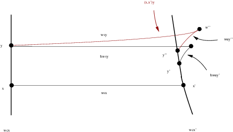
Hence we employ a different approach to prove that the holonomy maps are Hölder continuous. The proof here has some similarities with the proof that stable foliations are absolutely continuous. We fix two transversals τ\tau and τ′\tau^{\prime} to 𝒲ϕs\mathcal{W}^{s}_{\phi} and a pair of points x,y∈τx,y\in\tau. We iterate the picture forward until fϕn​(τ)f_{\phi}^{n}(\tau) and fϕn​(τ′)f_{\phi}^{n}(\tau^{\prime}) are very close and then push fϕn​(x)f_{\phi}^{n}(x) and fϕn​(y)f_{\phi}^{n}(y) across a short distance to points fϕn​(x′),fϕn​(y′)∈fϕn​(τ′)f_{\phi}^{n}(x^{\prime}),f_{\phi}^{n}(y^{\prime})\in f_{\phi}^{n}(\tau^{\prime}). The points x′,y′x^{\prime},y^{\prime} are the images of x,yx,y under 𝒲ϕs\mathcal{W}^{s}_{\phi}-holonomy; the iterate nn is chosen carefully so that the distance between xx and yy can be compared to some power of the distance between x′x^{\prime} and y′y^{\prime}. Unlike the proof of absolute continuity of stable foliations, in which nn is chosen arbitrarily large, the choice of nn is delicate and depends on the distance between xx and yy. We will employ this type of argument again in later sections.

As a final remark, we note that for every partially hyperbolic diffeomorphism ff and every Hölder continuous cocycle ϕ\phi, there is a choice of θ>0\theta>0 satisfying (16), for some Riemannian metric.

Proof of Proposition 5.2.

In this proof, we will use the convention that if qq is a point in MM and jj is an integer, then qjq_{j} denotes the point fj​(q)f^{j}(q), with q0=qq_{0}=q. If α:M→𝐑\alpha:M\to{\bf R} is a positive function, and j≥1j\geq 1 is an integer, we set

αj(p)=α(p)α(p1)⋯α(pj−1),\alpha_{j}(p)=\alpha(p)\alpha(p_{1})\cdots\alpha(p_{j-1}),

and

α−j(p)=α(p−j)−1α(p−j+1)−1⋯α(p−1)−1.\alpha_{-j}(p)=\alpha(p_{-j})^{-1}\alpha(p_{-j+1})^{-1}\cdots\alpha(p_{-1})^{-1}.

We set α0​(p)=1\alpha_{0}(p)=1. Observe that αj\alpha_{j} is a multiplicative cocycle; in particular, we have α−j​(p)−1=αj​(p−j)\alpha_{-j}(p)^{-1}=\alpha_{j}(p_{-j}). Note also that (α​β)j=αj​βj(\alpha\beta)_{j}=\alpha_{j}\beta_{j}, and if α\alpha is a constant function, then αn=αn\alpha_{n}=\alpha^{n}.

Fix θ∈(0,α]\theta\in(0,\alpha] satisfying (16). Next, fix a continuous positive function ρ:M→ℝ+\rho\colon M\to{\mathbb{R}}_{+} satisfying:

  • •

    ρ<min⁡{1,γ}\rho<\min\{1,\gamma\}, and

  • •

    ν​ρ−1≤(ν​μ^−1)θ/α\nu\rho^{-1}\leq(\nu\hat{\mu}^{-1})^{\theta/\alpha}.

We say that a smooth transversal Σ\Sigma to 𝒲s\mathcal{W}^{s} is admissible if the angle between T​ΣT\Sigma and EsE^{s} is at least π/4\pi/4.

The next lemma follows from an elementary inductive argument and continuity of the functions ν\nu, μ^\hat{\mu} and ρ\rho (cf. [BW2], Lemma 1.1).

Lemma 5.4.

There exists δ0>0\delta_{0}>0 such that for any p∈Mp\in M, and for any p′∈𝒲s​(p,δ0)p^{\prime}\in\mathcal{W}^{s}(p,\delta_{0}):

  1. (1)

    for any i≥0i\geq 0,

    d⁡(pi,pi′)≤νi​(p)​d​(p,p′);d(p_{i},p_{i}^{\prime})\leq\nu_{i}(p)d(p,p^{\prime});
  2. (2)

    for any admissible transversal Σ′\Sigma^{\prime} to 𝒲s\mathcal{W}^{s} at p′p^{\prime}, and any point q′∈Σ′q^{\prime}\in\Sigma^{\prime}, if d⁡(pi′,qi′)<δ0d(p_{i}^{\prime},q_{i}^{\prime})<\delta_{0}, for i=1,…,ni=1,\ldots,n, then

    ρi​(p)​d​(p′,q′)≤d⁡(pi′,qi′)≤μ^i​(p)−1​d​(p′,q′),\rho_{i}(p)d(p^{\prime},q^{\prime})\leq d(p_{i}^{\prime},q_{i}^{\prime})\leq\hat{\mu}_{i}(p)^{-1}d(p^{\prime},q^{\prime}),

    for i=1,…,ni=1,\ldots,n.

Let δ0>\delta_{0}> be given by this lemma; by rescaling the metric, we may assume that δ0=1\delta_{0}=1. Fix p∈Mp\in M and p′∈𝒲s​(p,1)p^{\prime}\in\mathcal{W}^{s}(p,1). Let Σ\Sigma and Σ′\Sigma^{\prime} be admissible transversals to 𝒲s\mathcal{W}^{s}, with p∈Σp\in\Sigma and p′∈Σ′p^{\prime}\in\Sigma^{\prime}, so that the 𝒲s\mathcal{W}^{s}-holonomy hs:Σ→Σ′h^{s}:\Sigma\to\Sigma^{\prime}, with hs​(p)=p′h^{s}(p)=p^{\prime} is well-defined. Let τ=Σ×ℝ\tau=\Sigma\times{\mathbb{R}}, and let τ′=Σ′×ℝ\tau^{\prime}=\Sigma^{\prime}\times{\mathbb{R}}. Fix q∈Σq\in\Sigma with d⁡(p,q)<1d(p,q)<1, and let q′=hs​(q)q^{\prime}=h^{s}(q).

For (z,t)∈M×ℝ(z,t)\in M\times{\mathbb{R}} and n≥0n\geq 0, write (zn,tn)(z_{n},t_{n}) for fϕn​(z,t)f_{\phi}^{n}(z,t). We introduce the notation Sn​ϕ​(z)=∑i=0n−1ϕ⁡(zi)S_{n}\phi(z)=\sum_{i=0}^{n-1}\phi(z_{i}), and note that S1​ϕ​(z)=ϕ⁡(z)S_{1}\phi(z)=\phi(z). With these notations, we have (zn,tn)=(zn,t+Sn​ϕ​(z))(z_{n},t_{n})=(z_{n},t+S_{n}\phi(z)). Denote by hϕs:Σ×ℝ→Σ×ℝh^{s}_{\phi}\colon\Sigma\times{\mathbb{R}}\to\Sigma\times{\mathbb{R}} the 𝒲ϕs\mathcal{W}^{s}_{\phi}-holonomy, which covers the map hsh^{s}. We first establish Hölder continuity of the base holonomy map hs:Σ→Σ′h^{s}\colon\Sigma\to\Sigma^{\prime}.

Since ν<μ^−1\nu<\hat{\mu}^{-1}, there exists an nn so that d⁡(p,q)=Θ⁡(νn​(p)​μ^n​(p))d(p,q)=\Theta(\nu_{n}(p)\hat{\mu}_{n}(p)); fix such an nn. Lemma 5.4 applied in the transversal Σ\Sigma implies that d⁡(pi,qi)≤μ^i​(p)−1​d​(p,q)≤O⁡(νn​(p))d(p_{i},q_{i})\leq\hat{\mu}_{i}(p)^{-1}d(p,q)\leq O(\nu_{n}(p)), for i=1,…,ni=1,\ldots,n.

On the other hand, since p′∈𝒲s​(p,1)p^{\prime}\in\mathcal{W}^{s}(p,1), we have d⁡(pi,pi′)≤O⁡(νi)d(p_{i},p^{\prime}_{i})\leq O(\nu_{i}), for all ii; in particular, d⁡(pn,pn′)≤O⁡(νn)d(p_{n},p^{\prime}_{n})\leq O(\nu_{n}). Similarly, (qn,qn′)≤O⁡(νn)(q_{n},q^{\prime}_{n})\leq O(\nu_{n}). By the triangle inequality, we have that

d⁡(pn′,qn′)\displaystyle d(p_{n}^{\prime},q_{n}^{\prime}) ≤\displaystyle\leq d⁡(pn,qn)+d⁡(pn,pn′)+d⁡(qn,qn′)\displaystyle d(p_{n},q_{n})+d(p_{n},p_{n}^{\prime})+d(q_{n},q_{n}^{\prime})
=\displaystyle= O​(νn​(p)).\displaystyle O(\nu_{n}(p)).

Now applying f−nf^{-n} to the pair of points pn′,qn′p_{n}^{\prime},q_{n}^{\prime} we obtain the pair of points p′,q′p^{\prime},q^{\prime}, which lie in the admissible transversal Σ′\Sigma^{\prime}. Lemma 5.4 then implies that d⁡(p′,q′)≤ρn​(p)−1​d​(pn′,qn′)≤O⁡(ρn​(p)−1​νn​(p))d(p^{\prime},q^{\prime})\leq\rho_{n}(p)^{-1}d(p_{n}^{\prime},q_{n}^{\prime})\leq O(\rho_{n}(p)^{-1}\nu_{n}(p)). Since ρn​(p)−1​νn​(p)<(νn​(p)​μ^n​(p))θ/α=O⁡(d​(p,q)θ/α)\rho_{n}(p)^{-1}\nu_{n}(p)<(\nu_{n}(p)\hat{\mu}_{n}(p))^{\theta/\alpha}=O(d(p,q)^{\theta/\alpha}), we obtain that d⁡(p′,q′)≤O⁡(d​(p,q)θ/α)≤O⁡(d​(p,q)θ)d(p^{\prime},q^{\prime})\leq O(d(p,q)^{\theta/\alpha})\leq O(d(p,q)^{\theta}), and so hsh^{s} is θ\theta-Hölder continuous.

We next turn to the Hölder continuity of hϕsh^{s}_{\phi}. Since hϕsh^{s}_{\phi} covers hsh^{s}, it suffices to establish Hölder continuity in the ℝ{\mathbb{R}}-fiber. Fix a point (p,r)∈Σ×ℝ(p,r)\in\Sigma\times{\mathbb{R}} and write hϕs​(p,r)=(p′,r′)h^{s}_{\phi}(p,r)=(p^{\prime},r^{\prime}) and hϕs​(q,s)=(q′,s′)h^{s}_{\phi}(q,s)=(q^{\prime},s^{\prime}).

Hölder continuity of ϕ\phi with exponent α\alpha implies that

|Sn​ϕ​(p)−Sn​ϕ​(q)|\displaystyle|S_{n}\phi(p)-S_{n}\phi(q)| ≤\displaystyle\leq ∑i=0n−1O⁡(d​(pi,qi)α)\displaystyle\sum_{i=0}^{n-1}O(d(p_{i},q_{i})^{\alpha})
≤\displaystyle\leq ∑i=0n−1O⁡((νn​(p)​μ^n​(p)​μ^i​(p)−1)α)\displaystyle\sum_{i=0}^{n-1}O((\nu_{n}(p)\hat{\mu}_{n}(p)\hat{\mu}_{i}(p)^{-1})^{\alpha})
=\displaystyle= νn​(p)α​∑i=0n−1O⁡(μ^−i​(pn)−α)\displaystyle\nu_{n}(p)^{\alpha}\sum_{i=0}^{n-1}O(\hat{\mu}_{-i}(p_{n})^{-\alpha})
≤\displaystyle\leq νn​(p)α​∑i=0n−1O⁡(μ¯i​α)=O⁡(νn​(p)α)\displaystyle\nu_{n}(p)^{\alpha}\sum_{i=0}^{n-1}O(\overline{\mu}^{i\alpha})=O(\nu_{n}(p)^{\alpha})

where μ¯<1\overline{\mu}<1 is an upper bound for μ^\hat{\mu}. This means that |rn−sn|≤|r−s|+O⁡(νn​(p)α)|r_{n}-s_{n}|\leq|r-s|+O(\nu_{n}(p)^{\alpha}).

Note that (pn′,rn′)∈𝒲ϕs​(pn,rn)(p_{n}^{\prime},r_{n}^{\prime})\in\mathcal{W}^{s}_{\phi}(p_{n},r_{n}). Proposition 3.1 implies that 𝒲ϕs​(pn,rn)\mathcal{W}^{s}_{\phi}(p_{n},r_{n}) is the graph of an α\alpha-Hölder continuous function from 𝒲s​(pn)\mathcal{W}^{s}(p_{n}) to ℝ{\mathbb{R}}. Hence

|rn−rn′|\displaystyle|r_{n}-r_{n}^{\prime}| ≤\displaystyle\leq O⁡(d​(pn,pn′)α)=O⁡(νn​(p)α),\displaystyle O(d(p_{n},p_{n}^{\prime})^{\alpha})=O(\nu_{n}(p)^{\alpha}),

and similarly, |sn−sn′|=O⁡(νn​(p)α)|s_{n}-s_{n}^{\prime}|=O(\nu_{n}(p)^{\alpha}). Now, by the triangle inequality,

(17) |rn′−sn′|\displaystyle|r_{n}^{\prime}-s_{n}^{\prime}| ≤\displaystyle\leq |rn−sn|+|rn−rn′|+|sn−sn′|\displaystyle|r_{n}-s_{n}|+|r_{n}-r_{n}^{\prime}|+|s_{n}-s_{n}^{\prime}|
(18) ≤\displaystyle\leq |r−s|+O⁡(νn​(p)α);\displaystyle|r-s|+O(\nu_{n}(p)^{\alpha});

Since d⁡(pn−i′,qn−i′)≤O⁡(νn​(p)​ρ−i​(pn))d(p_{n-i}^{\prime},q_{n-i}^{\prime})\leq O(\nu_{n}(p)\rho_{-i}(p_{n})), for i=1,…​ni=1,\ldots n, the α\alpha-Hölder continuity of ϕ\phi implies that |Snϕ(p′))−Snϕ(q′)|≤∑i=1nO((νn(p)ρ−i(pn))α)=O((νn(p)ρn(p)−1)α)|S_{n}\phi(p^{\prime}))-S_{n}\phi(q^{\prime})|\leq\sum_{i=1}^{n}O((\nu_{n}(p)\rho_{-i}(p_{n}))^{\alpha})=O((\nu_{n}(p)\rho_{n}(p)^{-1})^{\alpha}), since ρ<1\rho<1. The inequality (ν​ρ−1)α<(ν​μ^)θ(\nu\rho^{-1})^{\alpha}<(\nu\hat{\mu})^{\theta} now implies that

(19) |Snϕ(p′))−Snϕ(q′)|\displaystyle|S_{n}\phi(p^{\prime}))-S_{n}\phi(q^{\prime})| ≤\displaystyle\leq O⁡((νn​(p)​μ^n​(p))θ).\displaystyle O((\nu_{n}(p)\hat{\mu}_{n}(p))^{\theta}).

Combining (17) and (19), we obtain:

|r′−s′|\displaystyle|r^{\prime}-s^{\prime}| =\displaystyle= |(rn′−sn′)−(Snϕ(p′))−Snϕ(q′))|\displaystyle|(r_{n}^{\prime}-s_{n}^{\prime})-(S_{n}\phi(p^{\prime}))-S_{n}\phi(q^{\prime}))|
≤\displaystyle\leq |r−s|+O⁡(νn​(p)α)+O⁡((νn​(p)​μ^n​(p))θ)\displaystyle|r-s|+O(\nu_{n}(p)^{\alpha})+O((\nu_{n}(p)\hat{\mu}_{n}(p))^{\theta})
≤\displaystyle\leq |r−s|+O⁡((νn​(p)​μ^n​(p))θ),\displaystyle|r-s|+O((\nu_{n}(p)\hat{\mu}_{n}(p))^{\theta}),

since να<(ν​μ^)θ\nu^{\alpha}<(\nu\hat{\mu})^{\theta}.

We would like to compare |r′−s′||r^{\prime}-s^{\prime}| to d​((p,r),(q,s))θd((p,r),(q,s))^{\theta}; the latter quantity is equal to (|r−s|+d⁡(p,q))θ=(|r−s|+Θ⁡((νn​(p)​μ^n​(p))θ)CLOSE(|r-s|+d(p,q))^{\theta}=(|r-s|+\Theta((\nu_{n}(p)\hat{\mu}_{n}(p))^{\theta}); by the preceding calculation, |r′−s′|≤O⁡(d​((p,r),(q,s))θ)|r^{\prime}-s^{\prime}|\leq O(d((p,r),(q,s))^{\theta}). Hence hϕsh^{s}_{\phi} is θ\theta-Hölder continuous. ⋄\diamond

Having completed this preliminary step, we turn to the proof of the main result in this section.

Proof of Theorem A, part II.

Suppose that ff is accessible and ϕ:M→ℝ\phi\colon M\to{\mathbb{R}} is Hölder continuous. Let Φ:M→ℝ\Phi\colon M\to{\mathbb{R}} be a continuous map satisfying ϕ=Φ∘f−Φ+c\phi=\Phi\circ f-\Phi+c, for some c∈ℝc\in{\mathbb{R}}. We show that Φ\Phi is Hölder continuous. The key ingredient in the proof is the following lemma.

Lemma 5.5.

There exist C>0C>0, r0>0r_{0}>0 and κ∈(0,1)\kappa\in(0,1) with the following properties.

For any pair of points p,q∈Mp,q\in M, there exist functions α:BM​(p,r0)→BM​(q,1)\alpha\colon B_{M}(p,r_{0})\to B_{M}(q,1) and β:BM​(p,r0)→ℝ\beta\colon B_{M}(p,r_{0})\to{\mathbb{R}} with the following properties:

  1. (1)

    α⁡(p)=q\alpha(p)=q

  2. (2)

    for all z,z′∈BM​(p,r0)z,z^{\prime}\in B_{M}(p,r_{0}),

    d⁡(α⁡(z),α⁡(z′))≤C​d​(z,z′)κ,d(\alpha(z),\alpha(z^{\prime}))\leq Cd(z,z^{\prime})^{\kappa},

    and

    |β⁡(z)−β⁡(z′)|≤C​d​(z,z′)κ,|\beta(z)-\beta(z^{\prime})|\leq Cd(z,z^{\prime})^{\kappa},
  3. (3)

    for all z∈BM​(p,r0)z\in B_{M}(p,r_{0}), α⁡(z)\alpha(z) is the endpoint of an s​usu-path in MM originating at zz,

  4. (4)

    for all z∈BM​(p,r0)z\in B_{M}(p,r_{0}), and t∈ℝt\in{\mathbb{R}}, Δ⁡(z,t)\Delta(z,t) is the endpoint of an s​usu-lift path in M×ℝM\times{\mathbb{R}} originating at (z,t)(z,t), where Δ:BM​(p,r0)×ℝ→BM​(q,1)×ℝ\Delta\colon B_{M}(p,r_{0})\times{\mathbb{R}}\to B_{M}(q,1)\times{\mathbb{R}} is the map Δ⁡(z,t)=(α⁡(z),t+β⁡(z))\Delta(z,t)=(\alpha(z),t+\beta(z)).

Assuming this lemma, the proof proceeds as follows. Let C,r0,κC,r_{0},\kappa be given by Lemma 5.5. Fix x0,x1∈Mx_{0},x_{1}\in M with d⁡(x0,x1)<r0d(x_{0},x_{1})<r_{0}. For i≥1i\geq 1, we construct a sequence of points xix_{i} and maps αi:BM​(x0,r0)→BM​(xi,1)\alpha_{i}\colon B_{M}(x_{0},r_{0})\to B_{M}(x_{i},1), βi:BM​(x0,r0)→ℝ\beta_{i}\colon B_{M}(x_{0},r_{0})\to{\mathbb{R}} and Δi:BM​(x0,r0)×ℝ→BM​(xi,1)×ℝ\Delta_{i}\colon B_{M}(x_{0},r_{0})\times{\mathbb{R}}\to B_{M}(x_{i},1)\times{\mathbb{R}} inductively as follows. The point x1x_{1} is already defined. Assume that xix_{i}, for i≥1i\geq 1 has been defined. Let αi\alpha_{i} and βi\beta_{i} be given by the lemma, setting p=x0p=x_{0} and q=xiq=x_{i} (so that h⁡(x0)=xih(x_{0})=x_{i}). Define Δi\Delta_{i}, as in Lemma 5.5, by Δi​(z,t)=(αi​(z),t+βi​(z))\Delta_{i}(z,t)=(\alpha_{i}(z),t+\beta_{i}(z)). We then set xi+1=αi​(x1)x_{i+1}=\alpha_{i}(x_{1}).

We next argue that, for any i≥1i\geq 1, the map Δi\Delta_{i} has the property that, for all z∈BM​(x0,r0)z\in B_{M}(x_{0},r_{0}),

Δi​(z,Φ⁡(z))=(α⁡(z),Φ⁡(z)+βi​(z))=(α⁡(z),Φ⁡(α⁡(z))).\Delta_{i}(z,\Phi(z))=(\alpha(z),\Phi(z)+\beta_{i}(z))=(\alpha(z),\Phi(\alpha(z))).

Since Φ\Phi is a continuous solution to (2), Proposition 4.7 implies then the graph of Φ\Phi is bisaturated. That is, for any p,q∈Mp,q\in M, if (q,t)(q,t) is the endpoint of any s​u{su}-lift path originating at (p,Φ⁡(p))(p,\Phi(p)), then t=Φ⁡(q)t=\Phi(q). But properties 3 and 4 of the maps Δi\Delta_{i} given by Lemma 5.5 imply that αi​(z)\alpha_{i}(z) is the endpoint of an s​usu-path originating at zz, and Δi​(z,Φ​(z))\Delta_{i}(z,\Phi(z)) is the endpoint of an s​u{su}-lift path originating at (z,Φ⁡(z))(z,\Phi(z)). Hence we obtain that Δi​(z,Φ⁡(z))=(αi​(z),Φ⁡(αi​(z)))\Delta_{i}(z,\Phi(z))=(\alpha_{i}(z),\Phi(\alpha_{i}(z))), as claimed.

It now follows from the properties of Δi\Delta_{i} and the definition of xix_{i} that, for i≥1i\geq 1:

Φ⁡(x0)+βi​(x0)=Φ⁡(αi​(x0))=Φ⁡(xi),\Phi(x_{0})+\beta_{i}(x_{0})=\Phi(\alpha_{i}(x_{0}))=\Phi(x_{i}),

and

Φ⁡(x1)+βi​(x1)=Φ⁡(αi​(x1))=Φ⁡(xi+1).\Phi(x_{1})+\beta_{i}(x_{1})=\Phi(\alpha_{i}(x_{1}))=\Phi(x_{i+1}).

Thus:

(20) Φ⁡(x1)−Φ⁡(x0)\displaystyle\Phi(x_{1})-\Phi(x_{0}) =\displaystyle= (Φ⁡(xi+1)−Φ⁡(xi))+(βi​(x0)−βi​(x1)).\displaystyle\left(\Phi(x_{i+1})-\Phi(x_{i})\right)+\left(\beta_{i}(x_{0})-\beta_{i}(x_{1})\right).

Summing equation (20) over i∈{1,…,n}i\in\{1,\ldots,n\}, we obtain:

n⁡(Φ⁡(x1)−Φ⁡(x0))\displaystyle n\left(\Phi(x_{1})-\Phi(x_{0})\right) =\displaystyle= (Φ⁡(xn+1)−Φ⁡(x1))+∑i=1n(βi​(x0)−βi​(x1)),\displaystyle\left(\Phi(x_{n+1})-\Phi(x_{1})\right)+\sum_{i=1}^{n}\left(\beta_{i}(x_{0})-\beta_{i}(x_{1})\right),

and so:

|Φ⁡(x1)−Φ⁡(x0)|\displaystyle|\Phi(x_{1})-\Phi(x_{0})| ≤\displaystyle\leq 1n​|Φ⁡(xn+1)−Φ⁡(x1)|+1n​∑i=1n|βi​(x0)−βi​(x1)|\displaystyle\frac{1}{n}\left|\Phi(x_{n+1})-\Phi(x_{1})\right|+\frac{1}{n}\sum_{i=1}^{n}\left|\beta_{i}(x_{0})-\beta_{i}(x_{1})\right|
≤\displaystyle\leq 1n​‖ϕ‖∞+1n​∑i=1nC​d​(x0,x1)κ\displaystyle\frac{1}{n}\|\phi\|_{\infty}+\frac{1}{n}\sum_{i=1}^{n}Cd(x_{0},x_{1})^{\kappa}
≤\displaystyle\leq 1n​‖ϕ‖∞+C​d​(x0,x1)κ.\displaystyle\frac{1}{n}\|\phi\|_{\infty}+Cd(x_{0},x_{1})^{\kappa}.

Sending n→∞n\to\infty, we obtain that |Φ⁡(x1)−Φ⁡(x0)|≤C​d​(x0,x1)κ|\Phi(x_{1})-\Phi(x_{0})|\leq Cd(x_{0},x_{1})^{\kappa}; since x0x_{0} and x1x_{1} were arbitrary points within distance r0r_{0} of each other, this implies that Φ\Phi is κ\kappa-Hölder continuous. This completes the proof of Proposition 5.2, assuming Lemma 5.5. ⋄\diamond

Proof of Lemma 5.5.

Let θ\theta be given by Proposition 5.2, and let NMN_{M}, LML_{M} be given by Lemma 4.5.

We first describe how to construct the maps α\alpha and β\beta in the case where q∈𝒲s​(p,LM)q\in\mathcal{W}^{s}(p,L_{M}). The analogous construction works for q∈𝒲u​(p,LM)q\in\mathcal{W}^{u}(p,L_{M}). Lemma 4.5 implies that any pp and qq can be connected by an (KM,LM)(K_{M},L_{M})-accessible sequence. We can therefore construct α,β\alpha,\beta for a general pair of points pp and qq by composing at most KMK_{M} maps along stable and unstable segments.

Suppose then that p′∈𝒲s​(p,LM)p^{\prime}\in\mathcal{W}^{s}(p,L_{M}). We define α=αp,p′\alpha=\alpha_{p,p^{\prime}} as follows. Fix a foliation box UU of 𝒲s\mathcal{W}^{s} containing 𝒲s​(p,LM)\mathcal{W}^{s}(p,L_{M}), and let {Σx}x∈U\{\Sigma_{x}\}_{x\in U} be a (uniformly-chosen) smooth foliation by admissible transversals to 𝒲s\mathcal{W}^{s} in UU. For z∈Uz\in U, we define αp,p′​(z)\alpha_{p,p^{\prime}}(z) to be the unique point of intersection of 𝒲s​(z,LM)\mathcal{W}^{s}(z,L_{M}) with Σp′\Sigma_{p^{\prime}} in UU. The map αp,p′:U→Σp′\alpha_{p,p^{\prime}}\colon U\to\Sigma_{p^{\prime}} sends pp to p′p^{\prime} and is θ\theta-Hölder continuous when restricted to any transversal Σx\Sigma_{x}. Since {Σx}x∈𝒲s​(p)\{\Sigma_{x}\}_{x\in\mathcal{W}^{s}(p)} is a smooth foliation, it follows that αp,p′\alpha_{p,p^{\prime}} is θ\theta-Hölder continuous, uniformly in p′∈Up^{\prime}\in U.

Similarly, for (z,t)∈U×ℝ(z,t)\in U\times{\mathbb{R}}, we define Δp,p′​(z,t)\Delta_{p,p^{\prime}}(z,t) to be the unique point of intersection of 𝒲ϕs​(z)\mathcal{W}^{s}_{\phi}(z) with Σp′×ℝ\Sigma_{p^{\prime}}\times{\mathbb{R}} in U×ℝU\times{\mathbb{R}}. Proposition 3.1 implies that Δp,p′\Delta_{p,p^{\prime}} takes the form

Δp,p′​(z,t)=(αp,p′​(z),t+βp,p′​(z)),\Delta_{p,p^{\prime}}(z,t)=(\alpha_{p,p^{\prime}}(z),t+\beta_{p,p^{\prime}}(z)),

for some function βp,p′:U→ℝ\beta_{p,p^{\prime}}\colon U\to{\mathbb{R}}. Proposition 5.2 implies that Δp,p′\Delta_{p,p^{\prime}}, and so βp,p′\beta_{p,p^{\prime}}, is θ\theta-Hölder continuous, uniformly in p′∈Up^{\prime}\in U.

The same construction defines αp,p′\alpha_{p,p^{\prime}} and βp,p′\beta_{p,p^{\prime}} for p′∈𝒲u​(p,KM)p^{\prime}\in\mathcal{W}^{u}(p,K_{M}). Finally, for p,qp,q in MM, we fix an (KM,LM)(K_{M},L_{M})-accessible sequence (y0,y1,…,yKM)(y_{0},y_{1},\ldots,y_{K_{M}}) connecting pp and qq and define

αp,q=αyKM−1,yKM∘αyKM−2,yKM−1∘⋯∘αy0,y1.\alpha_{p,q}=\alpha_{y_{K_{M}-1},y_{K_{M}}}\circ\alpha_{y_{K_{M}-2},y_{K_{M}-1}}\circ\cdots\circ\alpha_{y_{0},y_{1}}.

By construction, αp,q​(p)=q\alpha_{p,q}(p)=q. Similarly define βp,q\beta_{p,q}.

Then there exists r0>0r_{0}>0 such that for every pair p,qp,q, αp,q\alpha_{p,q} and βp,q\beta_{p,q} are defined in the neighborhood BM​(p,r0)B_{M}(p,r_{0}) and αp,q\alpha_{p,q} takes values in BM​(q,1)B_{M}(q,1). Furthermore, there exists C>0C>0 such that (1) and (2) in the statement of the lemma hold, for κ=θKM\kappa=\theta^{K_{M}}. Finally, property (4) holds by construction.

⋄\diamond

Remark: The Hölder exponent for Φ\Phi obtained in this proof can be considerably smaller than the exponent for ϕ\phi. In particular, the largest possible exponent for the 𝒲ϕs\mathcal{W}^{s}_{\phi} or 𝒲ϕu\mathcal{W}^{u}_{\phi} holonomy given by Proposition 5.2 is 12\frac{1}{2}. Concatenating these holonomies along KK steps of an accessible sequence reduces this exponent further to 12K\frac{1}{2^{K}}. In contrast, the exponents for Φ\Phi and ϕ\phi in Theorem 0.1 are the same. This is because the transverse Hölder continuity of 𝒲ϕs\mathcal{W}^{s}_{\phi} and 𝒲ϕu\mathcal{W}^{u}_{\phi} does not play a role in the proof when ff is Anosov, and so only the Hölder exponent of the leaves, which is the same as for ϕ\phi, determines the exponent for Φ\Phi.

6. Jets

In this section we review basic facts about jets and jet bundles that will be needed in subsequent sections. The reader is referred to [H, KMS] for a more detailed account.

If N1N_{1} and N2N_{2} are CkC^{k} manifolds and ℓ≤k\ell\leq k, we denote by Γℓ​(N1,N2)\Gamma^{\ell}(N_{1},N_{2}) the set of local CkC^{k} maps from N1,N2N_{1},N_{2}; each element of Γℓ​(N1,N2)\Gamma^{\ell}(N_{1},N_{2}) is a triple (p,ϕ,U)(p,\phi,U), where ϕ\phi is a CℓC^{\ell} map from a neighborhood UU of pp in N1N_{1} to N2N_{2}. For p∈N1p\in N_{1}, we denote by Γpℓ​(N1,N2)\Gamma^{\ell}_{p}(N_{1},N_{2}) the set of elements of Γℓ​(N1,N2)\Gamma^{\ell}(N_{1},N_{2}) based at pp. We denote by Jℓ​(N1,N2)J^{\ell}(N_{1},N_{2}) the bundle of CℓC^{\ell} jets from N1N_{1} into N2N_{2}: each element of Jℓ​(N1,N2)J^{\ell}(N_{1},N_{2}) is an equivalence class of triples (p,ϕ,U)∈Γpℓ​(N1,N2)(p,\phi,U)\in\Gamma^{\ell}_{p}(N_{1},N_{2}), where two triples (p,ϕ,U)(p,\phi,U) and (p′,ϕ′,U′)(p^{\prime},\phi^{\prime},U^{\prime}) are equivalent if p=p′p=p^{\prime}, and the partials of ϕ\phi and ϕ′\phi^{\prime} at pp up to order ℓ\ell coincide.

We denote by [p,ϕ,U]ℓ[p,\phi,U]_{\ell} the equivalence class containing (p,ϕ,U)(p,\phi,U), which is called a ℓ\ell-jet at pp. Alternately, we use the notation jpℓ​ϕj^{\ell}_{p}\phi. The point pp is called the source of (p,ϕ,U)(p,\phi,U) and ϕ⁡(p)\phi(p) is the target. The source map σ\sigma gives Jℓ​(N1,N2)J^{\ell}(N_{1},N_{2}) the structure of a Ck−ℓC^{k-\ell} bundle over N1N_{1}; we denote by Jpℓ​(N1,N2)J^{\ell}_{p}(N_{1},N_{2}) the ℓ\ell-jets with source p∈N1p\in N_{1}. We also denote by Jℓ​(N1,N2)qJ^{\ell}(N_{1},N_{2})_{q} the set of jets with target qq.

More generally one has the ℓ\ell-jet bundle associated to a fiber bundle. If π:ℬ→M\pi\colon\mathcal{B}\to M is a CkC^{k} fiber bundle, and ℓ≤k\ell\leq k, we denote by Γℓ(π:ℬ→M)\Gamma^{\ell}(\pi\colon\mathcal{B}\to M) the set of CℓC^{\ell} local sections of ℬ\mathcal{B}, and by Γpℓ(π:ℬ→M)\Gamma^{\ell}_{p}(\pi\colon\mathcal{B}\to M) the set of CℓC^{\ell} local sections whose domain contains p∈Mp\in M. We then define the ℓ\ell-jet bundle Jℓ(π:ℬ→M)J^{\ell}(\pi\colon\mathcal{B}\to M) to be the set of pairs (p,ϕ)(p,\phi), where ϕ∈Γpr(π:ℬ→M)\phi\in\Gamma^{r}_{p}(\pi\colon\mathcal{B}\to M), and two pairs (p,ϕ)(p,\phi) and (p′,ϕ′)(p^{\prime},\phi^{\prime}) are equivalent if p=p′p=p^{\prime}, and the partials of ϕ\phi and ϕ′\phi^{\prime} at pp up to order ℓ\ell coincide. Then Jℓ(π:M→ℬ)J^{\ell}(\pi\colon M\to\mathcal{B}) is a Ck−ℓC^{k-\ell} bundle over MM. Observe that Jℓ(N1,N2)=Jℓ(projN1:N1×N2→N1)J^{\ell}(N_{1},N_{2})=J^{\ell}(\hbox{proj}_{N_{1}}\colon N_{1}\times N_{2}\to N_{1}) under the natural identification of sections of N1×N2N_{1}\times N_{2} with functions ϕ:N1→N2\phi:N_{1}\to N_{2}.

For ℓ′≤ℓ\ell^{\prime}\leq\ell, there is a natural projection πℓ,ℓ′\pi_{\ell,\ell^{\prime}} from the ℓ\ell-jet bundle to the ℓ′\ell^{\prime}-jet bundle that sends jpℓ​ϕj^{\ell}_{p}\phi to jpℓ′​ϕj^{\ell^{\prime}}_{p}\phi. Under this projection, JℓJ^{\ell} has the structure of a Ck−ℓ′C^{k-\ell^{\prime}} fiber bundle over Jℓ′J^{\ell^{\prime}}. Moreover, Jℓ−ℓ′​(Jℓ′)=JℓJ^{\ell-\ell^{\prime}}(J^{\ell^{\prime}})=J^{\ell}.

The bundle Jℓ​(ℝm,ℝn)J^{\ell}({\mathbb{R}}^{m},{\mathbb{R}}^{n}) is a trivial bundle over ℝm{\mathbb{R}}^{m}. The fiber space Jvℓ​(ℝm,ℝn)J^{\ell}_{v}({\mathbb{R}}^{m},{\mathbb{R}}^{n}) is the ℓ+1\ell+1-fold product Pℓ​(m,n)=Πi=0ℓ​Ls​y​mi​(ℝm,ℝn)P^{\ell}(m,n)=\Pi_{i=0}^{\ell}L^{i}_{sym}({\mathbb{R}}^{m},{\mathbb{R}}^{n}), where Ls​y​mi​(ℝm,ℝn)L^{i}_{sym}({\mathbb{R}}^{m},{\mathbb{R}}^{n}) is the vector space of of symmetric, ii-multilinear maps from ℝm{\mathbb{R}}^{m} to ℝn{\mathbb{R}}^{n}. Each ℓ\ell-jet [v,ϕ,U]ℓ[v,\phi,U]_{\ell} in Jvℓ​(ℝm,ℝn)J^{\ell}_{v}({\mathbb{R}}^{m},{\mathbb{R}}^{n}) has a canonical representative, which is the ℓ\ellth order Taylor polynomial of ϕ\phi about vv. To denote an element of Jℓ​(ℝm,ℝn)J^{\ell}({\mathbb{R}}^{m},{\mathbb{R}}^{n}), we sometimes use the notation (v,℘)(v,\wp) with v∈ℝmv\in{\mathbb{R}}^{m} and ℘\wp a degree ℓ\ell polynomial (suppressing the neighborhood UU, since polynomials are globally defined). These give C∞C^{\infty} global coordinates on Jℓ​(ℝm,ℝn)J^{\ell}({\mathbb{R}}^{m},{\mathbb{R}}^{n}); in this way we regard Jℓ​(ℝm,ℝn)J^{\ell}({\mathbb{R}}^{m},{\mathbb{R}}^{n}) as a finite dimensional vector space with a Euclidean structure |⋅||\cdot|.

6.1. Prolongations

If ϕ:N1→N2\phi:N_{1}\to N_{2} is a CℓC^{\ell} function, then ϕ\phi gives rise to a section of the bundle Jℓ​(N1,N2)J^{\ell}(N_{1},N_{2}) over N1N_{1} via the map v↦jvℓ​ϕv\mapsto j^{\ell}_{v}\phi. This section, denoted jℓ​ϕj^{\ell}\phi is called the ℓ\ell-prolongation of ϕ\phi. In the case ℓ=0\ell=0, the jet bundle J0​(N1,N2)J^{0}(N_{1},N_{2}) is just the product N1×N2N_{1}\times N_{2}, and the image of N1N_{1} under the prolongation j0​ϕj^{0}\phi is the just the graph of ϕ\phi.

The function ϕ:M→M\phi:M\to M is CkC^{k} if and only if the ℓ\ell-prolongation of ϕ\phi is Ck−ℓC^{k-\ell}. Not every continuous section of Jℓ​(M,N)J^{\ell}(M,N) is the prolongation of a CℓC^{\ell} function; however, the set of prolongations of smooth functions is closed:

Proposition 6.1.

If fn∈Cℓ​(M,N)f_{n}\in C^{\ell}(M,N) and jℓ​fn→jℓ​fj^{\ell}f_{n}\to j^{\ell}f in the weak topology on C0​(M,Jℓ​(M,N))C^{0}(M,J^{\ell}(M,N)), then f∈Cℓ​(M,N)f\in C^{\ell}(M,N).

More generally, if σ:M→ℬ\sigma\colon M\to\mathcal{B} is a section (resp. local section) of a CkC^{k} bundle π:ℬ→M\pi\colon\mathcal{B}\to M, then the ℓ\ell-prolongation jℓσ:M→Jℓ(π:M→ℬ)j^{\ell}\sigma\colon M\to J^{\ell}(\pi\colon M\to\mathcal{B}) is a Ck−ℓC^{k-\ell} section (resp. local section). The analogue of Proposition 6.1 holds for prolongations of sections.

6.2. Isomorphism of jet bundles

The next lemma is used extensively in various forms in this paper.

Lemma 6.2.

Let N1,N2,N_{1},N_{2}, and N3N_{3} be CkC^{k} manifolds.

  1. (1)

    Let g:N2→N3g:N_{2}\to N_{3} be a CkC^{k} map. Then for every ℓ≤k\ell\leq k, the map jxℓ​ϕ↦jxℓ​(g∘ϕ)j_{x}^{\ell}\phi\mapsto j_{x}^{\ell}(g\circ\phi) is a Ck−ℓC^{k-\ell} map from Jℓ​(N1,N2)J^{\ell}(N_{1},N_{2}) to Jℓ​(N1,N3)J^{\ell}(N_{1},N_{3}).

  2. (2)

    Let h:N1→N2h\colon N_{1}\to N_{2} be a CkC^{k} diffeomorphism. Then for every ℓ≤k\ell\leq k, the map jxℓ​ϕ↦jh⁡(x)ℓ​(ϕ∘h−1)j_{x}^{\ell}\phi\mapsto j_{h(x)}^{\ell}(\phi\circ h^{-1}) is a Ck−ℓC^{k-\ell} diffeomorphism from Jℓ​(N1,N3)J^{\ell}(N_{1},N_{3}) to Jℓ​(N2,N3)J^{\ell}(N_{2},N_{3}).

Remark: There is some subtlety in item 2. If h:N→Nh\colon N\to N is a Ck−ℓC^{k-\ell} diffeomorphism other than the identity, then neither of the following maps is even differentiable on Jℓ​(N,N)J^{\ell}(N,N):

jxℓ​ϕ↦jh⁡(x)ℓ​ϕorjxℓ​ϕ↦jxℓ​(ϕ∘h−1).j_{x}^{\ell}\phi\mapsto j_{h(x)}^{\ell}\phi\qquad\hbox{or}\quad j_{x}^{\ell}\phi\mapsto j_{x}^{\ell}(\phi\circ h^{-1}).

It is at first glance a fortuitous fact that the composition of these maps is Ck−ℓC^{k-\ell}. What item 2 expresses is the fact that the ℓ\ell-jet bundle is a Ck−ℓC^{k-\ell} invariant under CkC^{k}-diffeomorphisms. More generally:

Corollary 6.3.

(see, e.g. [KMS], Chapter 14.4) If π:ℬ→M\pi\colon\mathcal{B}\to M and π′:ℬ′→M′\pi^{\prime}\colon\mathcal{B}^{\prime}\to M^{\prime} are CkC^{k} fiber bundles, and H:ℬ→ℬ′H\colon\mathcal{B}\to\mathcal{B}^{\prime} is a CkC^{k} isomorphism of fiber bundles, covering the CkC^{k} diffeomorphism h:M→M′h\colon M\to M^{\prime}, then for every ℓ≤k\ell\leq k there is a canonical Ck−ℓC^{k-\ell} isomorphism of fiber bundles

Hℓ:Jℓ(π:ℬ→M)→Jℓ(π′:ℬ′→M′)H^{\ell}\colon J^{\ell}(\pi\colon\mathcal{B}\to M)\to J^{\ell}(\pi^{\prime}\colon\mathcal{B}^{\prime}\to M^{\prime})

covering hh. For ℓ′≤ℓ\ell^{\prime}\leq\ell, the map HℓH^{\ell} covers Hℓ′H^{\ell^{\prime}} under the natural projection.

The map HℓH^{\ell} is defined by:

Hℓ​(jxℓ​σ)=jh⁡(x)ℓ​(H∘σ∘h−1).H^{\ell}(j^{\ell}_{x}\sigma)=j_{h(x)}^{\ell}(H\circ\sigma\circ h^{-1}).

6.3. The graph transform on jets

In its local form, Corollary 6.3 tells us that for diffeomorphisms of ℝm×ℝn{\mathbb{R}}^{m}\times{\mathbb{R}}^{n} of the form H⁡(x,y)=(h⁡(x),g⁡(x,y))H(x,y)=(h(x),g(x,y)), the induced graph transform on functions Φ:ℝm→ℝn\Phi\colon{\mathbb{R}}^{m}\to{\mathbb{R}}^{n} produces a map that is smooth on the level of jets. By graph transform, we mean the map 𝒯H:{Φ:ℝm→ℝn}→{Φ:ℝm→ℝn}\mathcal{T}_{H}\colon\{\Phi\colon{\mathbb{R}}^{m}\to{\mathbb{R}}^{n}\}\to\{\Phi\colon{\mathbb{R}}^{m}\to{\mathbb{R}}^{n}\} defined by:

𝒯H​(Φ)​(x)=g⁡(h−1​(x),Φ⁡(h−1​(x))).\mathcal{T}_{H}(\Phi)(x)=g(h^{-1}(x),\Phi(h^{-1}(x))).

It is easy to see that if HH is CkC^{k}, then 𝒯H​(Cℓ​(ℝm,ℝn))=Cℓ​(ℝm,ℝn)\mathcal{T}_{H}(C^{\ell}({\mathbb{R}}^{m},{\mathbb{R}}^{n}))=C^{\ell}({\mathbb{R}}^{m},{\mathbb{R}}^{n}), for all ℓ≤k\ell\leq k; nonetheless, the restriction of 𝒯H\mathcal{T}_{H} to Cℓ​(ℝm,ℝn)C^{\ell}({\mathbb{R}}^{m},{\mathbb{R}}^{n}) is not smooth at all, even for ℓ=0\ell=0. What is smooth, however, is the induced map Hℓ:Jℓ​(ℝm,ℝn)→Jℓ​(ℝm,ℝn)H^{\ell}\colon J^{\ell}({\mathbb{R}}^{m},{\mathbb{R}}^{n})\to J^{\ell}({\mathbb{R}}^{m},{\mathbb{R}}^{n}):

Hℓ​(jxℓ​ψ)=jh⁡(x)ℓ​(𝒯H​(ψ)).H^{\ell}(j_{x}^{\ell}\psi)=j_{h(x)}^{\ell}(\mathcal{T}_{H}(\psi)).

This map on ℓ\ell-jets is Ck−ℓC^{k-\ell}.

More generally, whenever a graph transform is well-defined, it induces a continuous map on jets, which we now describe. Suppose that H⁡(x,y)=(h⁡(x,y),g⁡(x,y))H(x,y)=(h(x,y),g(x,y)) is a CkC^{k} local diffeomorphism of ℝm×ℝn{\mathbb{R}}^{m}\times{\mathbb{R}}^{n}. Write

Dv​H=(AvBvCvKv),D_{v}H=\left(\begin{array}[]{cc}A_{v}&B_{v}\\ C_{v}&K_{v}\end{array}\right),

where Av:ℝm→ℝmA_{v}\colon{\mathbb{R}}^{m}\to{\mathbb{R}}^{m}, Bv:ℝn→ℝmB_{v}\colon{\mathbb{R}}^{n}\to{\mathbb{R}}^{m}, Cv:ℝm→ℝnC_{v}\colon{\mathbb{R}}^{m}\to{\mathbb{R}}^{n} and Kv:ℝn→ℝnK_{v}\colon{\mathbb{R}}^{n}\to{\mathbb{R}}^{n}. Suppose that there exists ρ0>0\rho_{0}>0 such that for all v∈Bℝm+n​(0,ρ0)v\in B_{{\mathbb{R}}^{m+n}}(0,\rho_{0}), the map AvA_{v} is invertible.

Then there exists ρ1>0\rho_{1}>0 such that, for every ℓ≤k\ell\leq k, there exists a Ck−ℓC^{k-\ell} local diffeomorphism

Hℓ:Jℓ​(ℝm,ℝn)→Jℓ​(ℝm,ℝn),H^{\ell}\colon J^{\ell}({\mathbb{R}}^{m},{\mathbb{R}}^{n})\to J^{\ell}({\mathbb{R}}^{m},{\mathbb{R}}^{n}),

defined in the ρ1\rho_{1}-neighborhood of the 00-section of JBℝm​(0,ρ0)ℓ​(ℝm,ℝn)J^{\ell}_{B_{{\mathbb{R}}^{m}}(0,\rho_{0})}({\mathbb{R}}^{m},{\mathbb{R}}^{n}), given by:

Hℓ​(jxℓ​ψ)=jh⁡(x,ψ⁡(x))ℓ​((g∘(i​d,ψ))∘(h∘(i​d,ψ))−1).H^{\ell}(j^{\ell}_{x}\psi)=j^{\ell}_{h(x,\psi(x))}\left((g\circ(id,\psi))\circ(h\circ(id,\psi))^{-1}\right).

The map HℓH^{\ell} has the defining property that for every ψ∈Γℓ​(ℝm,ℝn)\psi\in\Gamma^{\ell}({\mathbb{R}}^{m},{\mathbb{R}}^{n}), if jxℓ​ψj_{x}^{\ell}\psi is in the domain of HℓH^{\ell}, and ψ′∈Γℓ​(ℝm,ℝn)\psi^{\prime}\in\Gamma^{\ell}({\mathbb{R}}^{m},{\mathbb{R}}^{n}) satisfies:

graph​(ψ′)=H⁡(graph​(ψ))\hbox{graph}(\psi^{\prime})=H(\hbox{graph}(\psi))

in a neighborhood of h⁡(x,ψ⁡(x))h(x,\psi(x)), then Hℓ​(jxℓ​ψ)=jh⁡(x,ψ⁡(x))ℓ​ψ′H^{\ell}(j^{\ell}_{x}\psi)=j_{h(x,\psi(x))}^{\ell}\psi^{\prime}. This fact motivates the term “graph transform.”

We explore the properties of these maps in more detail; this will be used in subsequent sections. Writing Pℓ​(m,n)=Πi=0ℓ​Ls​y​mi​(ℝm,ℝn)P^{\ell}(m,n)=\Pi_{i=0}^{\ell}L^{i}_{sym}({\mathbb{R}}^{m},{\mathbb{R}}^{n}), we have coordinates

(x,℘)↦(x,℘0,…,℘ℓ)(x,\wp)\mapsto(x,\wp_{0},\ldots,\wp_{\ell})

on ℝm×Pℓ​(m,n){\mathbb{R}}^{m}\times P^{\ell}(m,n), where ℘i=Dxi​℘∈Ls​y​mi​(ℝm,ℝn)\wp_{i}=D^{i}_{x}\wp\in L^{i}_{sym}({\mathbb{R}}^{m},{\mathbb{R}}^{n}). Denote by Hℓ​(x,℘)iH^{\ell}(x,\wp)_{i} the Ls​y​mi​(ℝm,ℝn)L^{i}_{sym}({\mathbb{R}}^{m},{\mathbb{R}}^{n})-coordinate of Hℓ​(x,℘)H^{\ell}(x,\wp), so that

Hℓ​(x,℘)=(h⁡(x,℘0),Hℓ​(x,℘)0,…,Hℓ​(x,℘)ℓ).H^{\ell}(x,\wp)=(h(x,\wp_{0}),H^{\ell}(x,\wp)_{0},\ldots,H^{\ell}(x,\wp)_{\ell}).

Clearly H0​(x,℘0)0=g⁡(x,℘0)H^{0}(x,\wp_{0})_{0}=g(x,\wp_{0}). Because jets are natural, for ℓ′≤ℓ\ell^{\prime}\leq\ell, we have

Hℓ​(x,℘0,…,℘ℓ)ℓ′=Hℓ′​(x,℘0,…,℘ℓ′)ℓ′.H^{\ell}(x,\wp_{0},\ldots,\wp_{\ell})_{\ell^{\prime}}=H^{\ell^{\prime}}(x,\wp_{0},\ldots,\wp_{\ell^{\prime}})_{\ell^{\prime}}.

Furthermore,

H1​(x,℘0,℘1)1=(C(x,℘0)+K(x,℘0)​℘1)​(A(x,℘0)+B(x,℘0)​℘1)−1.H^{1}(x,\wp_{0},\wp_{1})_{1}=\left(C_{(x,\wp_{0})}+K_{(x,\wp_{0})}\wp_{1}\right)\left(A_{(x,\wp_{0})}+B_{(x,\wp_{0})}\wp_{1}\right)^{-1}.

Differentiating this expression ℓ\ell times (implicitly), we get, for ℓ≥1\ell\geq 1:

Hℓ​(x,℘0,…,℘ℓ)ℓ\displaystyle H^{\ell}(x,\wp_{0},\ldots,\wp_{\ell})_{\ell} =\displaystyle= (K(x,℘0)​℘ℓ−H1​(v,℘0,℘1)1​B(x,℘0)​℘ℓCLOSE\displaystyle(K_{(x,\wp_{0})}\wp_{\ell}-H^{1}(v,\wp_{0},\wp_{1})_{1}B_{(x,\wp_{0})}\wp_{\ell}
OPEN+Sℓ​(x,℘0,…,℘ℓ−1))∘(A(x,℘0)+B(x,℘0)​℘1)−1,\displaystyle+S^{\ell}(x,\wp_{0},\ldots,\wp_{\ell-1}))\circ(A_{(x,\wp_{0})}+B_{(x,\wp_{0})}\wp_{1})^{-1},

where SℓS^{\ell} is a polynomial in (x,℘0,…,℘ℓ−1)(x,\wp_{0},\ldots,\wp_{\ell-1}) and in the partial derivatives of HH at (x,℘0)(x,\wp_{0}) up to order ℓ\ell.

Notice that if B(x,℘0)=0B_{(x,\wp_{0})}=0, then these expressions reduce to:

Hℓ​(x,℘0,…,℘ℓ)ℓ\displaystyle H^{\ell}(x,\wp_{0},\ldots,\wp_{\ell})_{\ell} =\displaystyle= (K(x,℘0)​℘ℓ+Sℓ​(x,℘0,…,℘ℓ−1))∘A(x,℘0)−1.\displaystyle(K_{(x,\wp_{0})}\wp_{\ell}+S^{\ell}(x,\wp_{0},\ldots,\wp_{\ell-1}))\circ A_{(x,\wp_{0})}^{-1}.

In particular, if B(x,℘0)=0B_{(x,\wp_{0})}=0, then there exists ρ2>0\rho_{2}>0 such that for all (x′,℘′)(x^{\prime},\wp^{\prime}) lying in the ρ2\rho_{2}-neighborhood of (x,℘)(x,\wp) in Jℓ​(ℝm,ℝn)J^{\ell}({\mathbb{R}}^{m},{\mathbb{R}}^{n}), we have:

(21) |Hℓ​(x,℘)ℓ−Hℓ​(x′,℘′)ℓ|\displaystyle|H^{\ell}(x,\wp)_{\ell}-H^{\ell}(x^{\prime},\wp^{\prime})_{\ell}|\qquad\qquad\qquad\qquad\qquad\qquad\qquad\qquad\qquad
(22) ≤Q(x,℘0)ℓ​(℘ℓ−℘ℓ′)+O⁡(|(x,℘0,…,℘ℓ−1)−(x′,℘0′,…,℘ℓ−1′)|),\displaystyle\qquad\quad\leq Q^{\ell}_{(x,\wp_{0})}(\wp_{\ell}-\wp_{\ell}^{\prime})+O\left(|(x,\wp_{0},\ldots,\wp_{\ell-1})-(x^{\prime},\wp_{0}^{\prime},\ldots,\wp_{\ell-1}^{\prime})|\right),

where Q(x,℘0)ℓ:Ls​y​mℓ​(ℝm,ℝn)→Ls​y​mℓ​(ℝm,ℝn)Q^{\ell}_{(x,\wp_{0})}\colon L^{\ell}_{sym}({\mathbb{R}}^{m},{\mathbb{R}}^{n})\to L^{\ell}_{sym}({\mathbb{R}}^{m},{\mathbb{R}}^{n}) is the linear map:

Q(x,℘0)ℓ​(℘¯ℓ)=K(x,℘0)∘℘¯ℓ∘A(x,℘0)−1.Q^{\ell}_{(x,\wp_{0})}(\overline{\wp}_{\ell})=K_{(x,\wp_{0})}\circ\overline{\wp}_{\ell}\circ A_{(x,\wp_{0})}^{-1}.

Observe that, because ℘¯ℓ\overline{\wp}_{\ell} is a symmetric map of order ℓ\ell, we have ‖Q(x,℘0)ℓ‖≤‖K(x,℘0)‖/m​(A(x,℘0))ℓ\|Q^{\ell}_{(x,\wp_{0})}\|\leq\|K_{(x,\wp_{0})}\|/m(A_{(x,\wp_{0})})^{\ell}, where m⁡(X)=‖X−1‖−1m(X)=\|X^{-1}\|^{-1} denotes the conorm of an invertible matrix XX.

For ℓ≥1\ell\geq 1, we may regard Jℓ​(ℝm,ℝn)J^{\ell}({\mathbb{R}}^{m},{\mathbb{R}}^{n}) as a vector bundle over J0​(ℝm,ℝn)J^{0}({\mathbb{R}}^{m},{\mathbb{R}}^{n}) (=ℝm×ℝn={\mathbb{R}}^{m}\times{\mathbb{R}}^{n}) under the natural projection πℓ,0\pi_{\ell,0}; the fiber is Πi=1ℓ​Ls​y​mi​(ℝm,ℝn)\Pi_{i=1}^{\ell}L^{i}_{sym}({\mathbb{R}}^{m},{\mathbb{R}}^{n}). In a variety of contexts (see Section 10.1 ff.) we will consider the case where the map HℓH^{\ell} is a fiberwise contraction on a neighborhood of the 00-section of this bundle. We assume that ‖K(x,℘0)‖<m⁡(A(x,℘0))\|K_{(x,\wp_{0})}\|<m(A_{(x,\wp_{0})}) and ‖K(x,℘0)‖<m​(A(x,℘0))ℓ\|K_{(x,\wp_{0})}\|<m(A_{(x,\wp_{0})})^{\ell} (which together imply that ‖K(x,℘0)‖<m​(A(x,℘0))i\|K_{(x,\wp_{0})}\|<m(A_{(x,\wp_{0})})^{i}, for 1≤i≤ℓ1\leq i\leq\ell).

Continuing to assume that B(x,℘0)=0B_{(x,\wp_{0})}=0, we next construct in the standard way a norm |⋅|′|\cdot|^{\prime} on Πi=1ℓ​Ls​y​mi​(ℝm,ℝn)\Pi_{i=1}^{\ell}L^{i}_{sym}({\mathbb{R}}^{m},{\mathbb{R}}^{n}) such that:

(23) |Hℓ​(x,℘)−Hℓ​(x,℘′)|′\displaystyle|H^{\ell}(x,\wp)-H^{\ell}(x,\wp^{\prime})|^{\prime}\qquad\qquad\qquad\qquad\qquad\qquad\qquad\qquad\qquad\quad
(24) ≤max⁡{‖A(x,℘0)‖m⁡(K(x,℘0)),‖K(x,℘0)‖m​(A(x,℘0))ℓ}⋅|(x,℘)ℓ−(x,℘′)ℓ|′,\displaystyle\qquad\qquad\qquad\qquad\leq\max\left\{\frac{\|A_{(x,\wp_{0})}\|}{m(K_{(x,\wp_{0})})},\frac{\|K_{(x,\wp_{0})}\|}{m(A_{(x,\wp_{0})})^{\ell}}\right\}\cdot|(x,\wp)_{\ell}-(x,\wp^{\prime})_{\ell}|^{\prime},

for (x,℘),(x,℘′)(x,\wp),(x,\wp^{\prime}) lying in the set {(x,℘0,℘¯1,…,℘¯ℓ):|(℘¯1,…,℘¯ℓ)|′≤1}\{(x,\wp_{0},\overline{\wp}_{1},\ldots,\overline{\wp}_{\ell})\colon|(\overline{\wp}_{1},\ldots,\overline{\wp}_{\ell})|^{\prime}\leq 1\}. To do this, fix L>0L>0 and for (℘¯1,…,℘¯ℓ)∈Πi=1ℓ​Ls​y​mi​(ℝm,ℝn)(\overline{\wp}_{1},\ldots,\overline{\wp}_{\ell})\in\Pi_{i=1}^{\ell}L^{i}_{sym}({\mathbb{R}}^{m},{\mathbb{R}}^{n}), define:

|(℘¯1,…,℘¯ℓ)|L=Lℓ​|℘¯1|+⋯+L​|℘¯ℓ|.|(\overline{\wp}_{1},\ldots,\overline{\wp}_{\ell})|_{L}=L^{\ell}|\overline{\wp}_{1}|+\cdots+L|\overline{\wp}_{\ell}|.

It is not difficult to verify using (21) that if L>0L>0 is sufficiently large, then (23) holds for |⋅|′=|⋅|L|\cdot|^{\prime}=|\cdot|_{L} and all (x,℘),(x,℘′)(x,\wp),(x,\wp^{\prime}) lying in the set {(x,℘0,℘¯1,…,℘¯ℓ):|(℘¯1,…,℘¯ℓ)|′≤1}\{(x,\wp_{0},\overline{\wp}_{1},\ldots,\overline{\wp}_{\ell})\colon|(\overline{\wp}_{1},\ldots,\overline{\wp}_{\ell})|^{\prime}\leq 1\}.

The same holds true if ‖B(x,℘0)‖\|B_{(x,\wp_{0})}\| is sufficiently small. Summarizing this discussion, we have:

Lemma 6.4.

Fix ℓ≥1\ell\geq 1. For every R>0R>0 and κ∈(0,1)\kappa\in(0,1) there exist ε>0\varepsilon>0 and L>0L>0 with the following properties.

Let H:Bℝm+n​(0,1)→ℝm+nH\colon B_{{\mathbb{R}}^{m+n}}(0,1)\to{\mathbb{R}}^{m+n} be a CℓC^{\ell} local diffeomorphism such that:

  • •

    dCℓ​(H,I​d)≤Rd_{C^{\ell}}(H,Id)\leq R, and

  • •

    writing Dv​H=(AvBvCvKv)D_{v}H=\left(\begin{array}[]{cc}A_{v}&B_{v}\\ C_{v}&K_{v}\end{array}\right), we have:

    infv∈Bℝm+n​(0,1)m⁡(Av)>0,\inf_{v\in B_{{\mathbb{R}}^{m+n}}(0,1)}m(A_{v})>0,
    κ>supv∈Bℝm+n​(0,1)max⁡{‖Kv‖m⁡(Av),‖Kv‖m​(Av)ℓ},\kappa>\sup_{v\in B_{{\mathbb{R}}^{m+n}}(0,1)}\max\left\{\frac{\|K_{v}\|}{m(A_{v})},\frac{\|K_{v}\|}{m(A_{v})^{\ell}}\right\},

    and

    supv∈Bℝm+n​(0,1)‖Bv‖<ε.\sup_{v\in B_{{\mathbb{R}}^{m+n}}(0,1)}\|B_{v}\|<\varepsilon.

Then for all v=(vm,vn)∈ℝm+nv=(v^{m},v^{n})\in{\mathbb{R}}^{m+n} and all jvmℓ​ψ,jvmℓ​ψ′∈πℓ,0−1​(v)j_{v^{m}}^{\ell}\psi,j_{v^{m}}^{\ell}\psi^{\prime}\in\pi_{\ell,0}^{-1}(v), with |jvmℓ​ψ|,|jvmℓ​ψ′|≤1|j_{v^{m}}^{\ell}\psi|,|j^{\ell}_{v^{m}}\psi^{\prime}|\leq 1, we have:

|Hℓ​(jvmℓ​ψ)−Hℓ​(jvmℓ​ψ′)|L≤κ​|jvmℓ​ψ−jvmℓ​ψ′|L.|H^{\ell}(j^{\ell}_{v^{m}}\psi)-H^{\ell}(j^{\ell}_{v^{m}}\psi^{\prime})|_{L}\leq\kappa|j^{\ell}_{v^{m}}\psi-j^{\ell}_{v^{m}}\psi^{\prime}|_{L}.

7. Proof of Theorem B

Before proving our main higher regularity result (part IV of Theorem A), we give a proof of Theorem B, as the proof conveys some of the basic techniques we will use later, but in a simpler setting.

Suppose that NN is an embedded C1C^{1} submanifold of ℝm+n{\mathbb{R}}^{m+n} such that, for every x,yx,y in NN, there exist neighborhoods UU of xx and VV of yy and a CkC^{k} diffeomorphism H:U→VH:U\to V such that H⁡(U)=VH(U)=V and H⁡(U∩N)=V∩NH(U\cap N)=V\cap N, where k≥2k\geq 2.

We prove that NN is a CℓC^{\ell} submanifold of ℝm+n{\mathbb{R}}^{m+n}, for all ℓ≤k\ell\leq k, by induction on ℓ\ell. By assumption, NN is a C1C^{1} submanifold. Suppose that NN is a CℓC^{\ell} submanifold, for some ℓ≤k−1\ell\leq k-1. We prove that NN is Cℓ+1C^{\ell+1} submanifold. As the problem is local, we may restrict attention to a small neighborhood in NN.

Fix a point x0∈Nx_{0}\in N and a neighborhood VV of x0x_{0} in NN. By a local CkC^{k} change of coordinates in N′N^{\prime} sending x0x_{0} to 0∈ℝn×ℝm0\in{\mathbb{R}}^{n}\times{\mathbb{R}}^{m}, we may assume that NN is the graph of a CℓC^{\ell} function Φ:Bℝn​(0,1)¯→ℝm\Phi:\overline{B_{{\mathbb{R}}^{n}}(0,1)}\to{\mathbb{R}}^{m} satisfying j0k​Φ=0j^{k}_{0}\Phi=0. The first main step in the proof of Theorem B is the following lemma.

Lemma 7.1.

For every u∈Bℝn​(0,1)¯u\in\overline{B_{{\mathbb{R}}^{n}}(0,1)} there exists ρ=ρ⁡(u)>0\rho=\rho(u)>0, and for every i∈{0,…,ℓ}i\in\{0,\ldots,\ell\}, a Ck−iC^{k-i} local diffeomorphism

Hui:BJi​(ℝn,ℝm)​(0,ρ)→Ji​(ℝn,ℝm)H_{u}^{i}\colon B_{J^{i}({\mathbb{R}}^{n},{\mathbb{R}}^{m})}(0,\rho)\to J^{i}({\mathbb{R}}^{n},{\mathbb{R}}^{m})

with the following properties:

  1. (1)

    HuiH_{u}^{i} covers Hui−1H_{u}^{i-1} under the projection Ji​(ℝn,ℝm)→Ji−1​(ℝn,ℝm)J^{i}({\mathbb{R}}^{n},{\mathbb{R}}^{m})\to J^{i-1}({\mathbb{R}}^{n},{\mathbb{R}}^{m}), and

  2. (2)

    writing Hu0​(v,w)=(hu​(v,w),gu​(v,w))H_{u}^{0}(v,w)=(h_{u}(v,w),g_{u}(v,w)), we have hu​(0,Φ⁡(0))=uh_{u}(0,\Phi(0))=u, and:

    Huℓ​(jvℓ​Φ)=jhu​(v,Φ​(v))ℓ​Φ,H_{u}^{\ell}(j^{\ell}_{v}\Phi)=j_{h_{u}(v,\Phi(v))}^{\ell}\Phi,

    for every vv such that jvℓ​Φ∈BJℓ​(ℝn,ℝm)​(0,ρ)j^{\ell}_{v}\Phi\in B_{J^{\ell}({\mathbb{R}}^{n},{\mathbb{R}}^{m})}(0,\rho).

Proof.

For i=0i=0, this follows immediately from CkC^{k} homogeneity. Given u∈Bℝn​(0,1)¯u\in\overline{B_{{\mathbb{R}}^{n}}(0,1)}, select a CkC^{k} local diffeomorphism

Hu=(hu,gu):Bℝn×ℝm​(0,ρ0)→ℝn×ℝmH_{u}=(h_{u},g_{u})\colon B_{{\mathbb{R}}^{n}\times{\mathbb{R}}^{m}}(0,\rho_{0})\to{\mathbb{R}}^{n}\times{\mathbb{R}}^{m}

sending (0,0)=(0,Φ⁡(0))(0,0)=(0,\Phi(0)) to (u,Φ⁡(u))(u,\Phi(u)) and preserving the graph of Φ\Phi. Under the natural identification of J0​(ℝn,ℝm)J^{0}({\mathbb{R}}^{n},{\mathbb{R}}^{m}) with ℝn×ℝm{\mathbb{R}}^{n}\times{\mathbb{R}}^{m}, this defines the map Hu0H^{0}_{u}:

Hu0​(v,w)=(hu​(v,w),gu​(v,w)).H^{0}_{u}(v,w)=(h_{u}(v,w),g_{u}(v,w)).

Suppose i≥1i\geq 1, and fix a point v′∈ℝnv^{\prime}\in{\mathbb{R}}^{n} near 00, and a function ψ∈Γv′i​(ℝn,ℝm)\psi\in\Gamma^{i}_{v^{\prime}}({\mathbb{R}}^{n},{\mathbb{R}}^{m}). Consider the local map hu∘(i​d,ψ)∈Γv′i​(ℝn,ℝn)h_{u}\circ(id,\psi)\in\Gamma^{i}_{v^{\prime}}({\mathbb{R}}^{n},{\mathbb{R}}^{n}) given by:

Hu∘(i​d,ψ)​(v)=hu​(v,ψ⁡(v)).H_{u}\circ(id,\psi)(v)=h_{u}(v,\psi(v)).

Its derivative at v′v^{\prime} is

(25) Dv′​(hu∘(i​d,ψ))=∂hu∂v​(v′,ψ⁡(v′))+∂hu∂w​(v′,ψ⁡(v′))​Dv′​ψ.\displaystyle D_{v^{\prime}}\left(h_{u}\circ(id,\psi)\right)=\frac{\partial h_{u}}{\partial v}(v^{\prime},\psi(v^{\prime}))+\frac{\partial h_{u}}{\partial w}(v^{\prime},\psi(v^{\prime}))D_{v^{\prime}}\psi.

Since D​Hu0DH^{0}_{u} preserves the tangent space to the graph of Φ\Phi, it follows that the map ∂Hu/∂v⁡(0,0){\partial H_{u}}/{\partial v}(0,0) is a diffeomorphism onto a neighborhood of uu. On the other hand, plugging in v′=0{v^{\prime}}=0, Dv′​ψ=0D_{v^{\prime}}\psi=0 into equation (25) we obtain that for any ψ∈Γ0i​(ℝn,ℝm)\psi\in\Gamma^{i}_{0}({\mathbb{R}}^{n},{\mathbb{R}}^{m}) with j01​ψ=0j^{1}_{0}\psi=0, D0​(hu∘(i​d,ψ))=∂hu∂v​(0,0)D_{0}\left(h_{u}\circ(id,\psi)\right)=\frac{\partial h_{u}}{\partial v}(0,0).

Since H0H^{0} is C1C^{1}, from this it follows that for |jv′i​ψ||j^{i}_{v^{\prime}}\psi| and |v′||v^{\prime}| sufficiently small, the derivative Dv′​(hu∘(i​d,ψ))D_{v^{\prime}}\left(h_{u}\circ(id,\psi)\right) is invertible. The inverse function theorem then implies that hu∘(i​d,ψ)h_{u}\circ(id,\psi) is a CiC^{i} local diffeomorphism in a neighborhood of v∈ℝnv\in{\mathbb{R}}^{n}, provided |jvi​ψ||j_{v}^{i}\psi| is sufficiently small; in particular, (hu∘(i​d,ψ))−1(h_{u}\circ(id,\psi))^{-1} is defined.

For i≥1i\geq 1, we then set

Hui​(jvi​ψ)=jhu​(v,ψ​(v))i​((gu∘(i​d,ψ))∘(hu∘(i​d,ψ))−1).H^{i}_{u}(j^{i}_{v}\psi)=j^{i}_{h_{u}(v,\psi(v))}\left((g_{u}\circ(id,\psi))\circ(h_{u}\circ(id,\psi))^{-1}\right).

Lemma 6.2 implies that HuiH^{i}_{u} is a Ck−iC^{k-i} local diffeomorphism. By construction, the maps HuiH_{u}^{i} satisfy properties (1) and (2). ⋄\diamond

Remark: Notice that Lemma 7.1 implies that the image of Bℝn​(0,1)¯\overline{B_{{\mathbb{R}}^{n}}(0,1)} under jℓ​Φj^{\ell}\Phi is a C1C^{1} homogeneous submanifold of Jℓ​(ℝn,ℝm)J^{\ell}({\mathbb{R}}^{n},{\mathbb{R}}^{m}). At this point, it is tempting to appeal to Theorem 1.2 to finish the proof. If one does so, one obtains that jℓ​Φ​(Bℝn​(0,1)¯)j^{\ell}\Phi(\overline{B_{{\mathbb{R}}^{n}}(0,1)}) is a C1C^{1} submanifold of Jℓ​(ℝn,ℝm)J^{\ell}({\mathbb{R}}^{n},{\mathbb{R}}^{m}). However, this alone does not imply that Φ\Phi is Cℓ+1C^{\ell+1}. To conclude that Φ\Phi is Cℓ+1C^{\ell+1}, for ℓ≥1\ell\geq 1, it is in fact necessary to show that the function jℓ​Φj^{\ell}\Phi, and not just its image, is C1C^{1}.

Here is an example that illustrates what can go wrong. Let Ψ:ℝ→ℝ\Psi\colon{\mathbb{R}}\to{\mathbb{R}} be any C2C^{2} function, and let Φ⁡(x)=Ψ⁡(x)+x4/3\Phi(x)=\Psi(x)+x^{4/3}. Then the graph of Φ\Phi is a C1C^{1} submanifold of ℝ2{\mathbb{R}}^{2}, but not a C2C^{2} submanifold, as is easily checked. On the other hand, jx1​Φ=(x,Ψ⁡(x)+x4/3,Ψ′​(x)+(4/3)​x1/3)j^{1}_{x}\Phi=(x,\Psi(x)+x^{4/3},\Psi^{\prime}(x)+(4/3)x^{1/3}), and the image of j1​Φj^{1}\Phi is the image of the following C1C^{1} embedding:

ψ:ℝ→ℝ3;ψ⁡(t)=(t3,Ψ⁡(t3)+t4,Ψ′​(t3)+(4/3)​t).\psi\colon{\mathbb{R}}\to{\mathbb{R}}^{3};\quad\psi(t)=(t^{3},\Psi(t^{3})+t^{4},\Psi^{\prime}(t^{3})+(4/3)t).

Hence the image of j1​Φj^{1}\Phi is C1C^{1}, but the graph of Φ\Phi is not C2C^{2}.

The situation can be arbitrarily bad: if Ψ\Psi is real analytic, then the image of j1​Φj^{1}\Phi is analytic, while the graph of Φ\Phi still fails to be C2C^{2}. (The construction we have described is a very simple example of the procedure in algebraic geometry of resolving a singularity.)

Returning to the proof of Theorem B, our next step is to show:

If Φ\Phi is CℓC^{\ell} and jℓ​Φj^{\ell}\Phi is a C1C^{1}-homogeneous function (in the sense of
Lemma 7.1), then jℓ​Φj^{\ell}\Phi is C1C^{1}, and so Φ\Phi is Cℓ+1C^{\ell+1}.

To this end, let A:Jℓ​(ℝn,ℝm)→Jℓ​(ℝn,ℝm)A\colon J^{\ell}({\mathbb{R}}^{n},{\mathbb{R}}^{m})\to J^{\ell}({\mathbb{R}}^{n},{\mathbb{R}}^{m}) be an invertible linear transformation, and let ρ>0\rho>0. We next define a subset 𝒢⁡(A,ρ)⊂Bℝn​(0,1)¯\mathcal{G}(A,\rho)\subset\overline{B_{{\mathbb{R}}^{n}}(0,1)} consisting of the set of all u∈Bℝn​(0,1)¯u\in\overline{B_{{\mathbb{R}}^{n}}(0,1)} with the following properties:

  • •

    For each i∈{0,…​ℓ}i\in\{0,\ldots\ell\}, there exists a bilipschitz embedding

    H~ui:BJi​(ℝn,ℝm)​(0,ρ)→Ji​(ℝn,ℝm)\tilde{H}_{u}^{i}\colon B_{J^{i}({\mathbb{R}}^{n},{\mathbb{R}}^{m})}(0,\rho)\to J^{i}({\mathbb{R}}^{n},{\mathbb{R}}^{m})

    such that:

  • •

    H~ui\tilde{H}_{u}^{i} covers H~ui−1\tilde{H}_{u}^{i-1} under the projection Ji​(ℝn,ℝm)→Ji−1​(ℝn,ℝm)J^{i}({\mathbb{R}}^{n},{\mathbb{R}}^{m})\to J^{i-1}({\mathbb{R}}^{n},{\mathbb{R}}^{m}),

  • •

    writing H~u0​(v,w)=(h~u​(v,w),g~u​(v,w))\tilde{H}_{u}^{0}(v,w)=(\tilde{h}_{u}(v,w),\tilde{g}_{u}(v,w)), we have h~u​(0,Φ⁡(0))=u\tilde{h}_{u}(0,\Phi(0))=u, and:

    H~uℓ​(jvℓ​Φ)=jh~u​(v,Φ​(v))​Φ,\tilde{H}_{u}^{\ell}(j^{\ell}_{v}\Phi)=j_{\tilde{h}_{u}(v,\Phi(v))}\Phi,

    for every vv such that jvℓ​Φ∈BJℓ​(ℝn,ℝm)​(0,ρ)j^{\ell}_{v}\Phi\in B_{J^{\ell}({\mathbb{R}}^{n},{\mathbb{R}}^{m})}(0,\rho), and

  • •

    Lip​(A−H~uℓ)≤m⁡(A)5\hbox{Lip}(A-\tilde{H}^{\ell}_{u})\leq\frac{m(A)}{5} on BJℓ​(ℝn,ℝm)​(0,ρ)B_{J^{\ell}({\mathbb{R}}^{n},{\mathbb{R}}^{m})}(0,\rho), where m⁡(A)=‖A−1‖−1m(A)=\|A^{-1}\|^{-1} denotes the conorm of AA.

Fix a countable dense subset {Aj}j∈ℤ+⊂G​L​(Jℓ​(ℝn,ℝm))\{A_{j}\}_{j\in{\mathbb{Z}}_{+}}\subset GL(J^{\ell}({\mathbb{R}}^{n},{\mathbb{R}}^{m})) of invertible linear transformations.

Lemma 7.2.

For each A∈G​L​(Jℓ​(ℝm,ℝn))A\in GL(J^{\ell}({\mathbb{R}}^{m},{\mathbb{R}}^{n})), and ρ>0\rho>0, the set 𝒢⁡(A,ρ)\mathcal{G}(A,\rho) is compact in Bℝn​(0,1)¯\overline{B_{{\mathbb{R}}^{n}}(0,1)}. Moreover:

Bℝn​(0,1)¯=⋃j1,j2∈ℤ+𝒢⁡(Aj1,j2−1).\overline{B_{{\mathbb{R}}^{n}}(0,1)}=\bigcup_{j_{1},j_{2}\in{\mathbb{Z}}_{+}}\mathcal{G}(A_{j_{1}},j_{2}^{-1}).
Proof.

Suppose that 𝒢⁡(A,ρ)\mathcal{G}(A,\rho) is nonempty. Let uju_{j} be a sequence in 𝒢⁡(A,ρ)\mathcal{G}(A,\rho), and for each i∈{0,…,ℓ}i\in\{0,\ldots,\ell\}, let H~uji\tilde{H}^{i}_{u_{j}} be the associated sequence of bilipschitz embeddings. Since the space of bilipschitz embeddings is locally compact in the uniform topology, there exists a convergent subsequence ujℓ→u∈Bℝn​(0,1)¯u_{j_{\ell}}\to u\in\overline{B_{{\mathbb{R}}^{n}}(0,1)} with H~ujℓi→H~ui\tilde{H}^{i}_{u_{j_{\ell}}}\to\tilde{H}^{i}_{u} uniformly for all ii. The maps H~ui\tilde{H}^{i}_{u} are bilipschitz embeddings, with H~ui\tilde{H}^{i}_{u} covering H~ui−1\tilde{H}^{i-1}_{u}, and Lip​(Hui−A)≤m⁡(A)5\hbox{Lip}(H^{i}_{u}-A)\leq\frac{m(A)}{5}. Since the ℓ\ell-jet jℓ​Φj^{\ell}\Phi is a closed subset of Jℓ​(ℝn,ℝm)J^{\ell}({\mathbb{R}}^{n},{\mathbb{R}}^{m}), the limiting map H~uℓ\tilde{H}^{\ell}_{u} preserves jℓ​Φj^{\ell}\Phi. Hence u∈𝒢⁡(A,ρ)u\in\mathcal{G}(A,\rho), and so 𝒢⁡(A,ρ)\mathcal{G}(A,\rho) is compact.

Lemma 7.1 implies that for each uu, and each ii there exists a Cr−iC^{r-i} diffeomorphism HuiH^{i}_{u} satisfying the first two properties. Let ε=m⁡(D0​Huℓ)/11\varepsilon=m(D_{0}H^{\ell}_{u})/11. Fix Aj1∈G​L​(Jℓ​(ℝn,ℝm))A_{j_{1}}\in GL(J^{\ell}({\mathbb{R}}^{n},{\mathbb{R}}^{m})) such that ‖D0​Huℓ−Aj1‖<ε\|D_{0}H^{\ell}_{u}-A_{j_{1}}\|<\varepsilon. A simple estimate shows that ‖D0​Huℓ−Aj1‖<m⁡(Aj1)10\|D_{0}H^{\ell}_{u}-A_{j_{1}}\|<\frac{m(A_{j_{1}})}{10}. Next, fix j2j_{2} such that Lip​(D0​Huℓ−Huℓ)<m⁡(Aj1)10\hbox{Lip}(D_{0}H^{\ell}_{u}-H^{\ell}_{u})<\frac{m(A_{j_{1}})}{10} on BJℓ​(ℝm,ℝn)​(0,j2−1)B_{J^{\ell}({\mathbb{R}}^{m},{\mathbb{R}}^{n})}(0,j_{2}^{-1}). Then Lip​(Aj1−Huℓ)<m⁡(Aj1)5\hbox{Lip}(A_{j_{1}}-H^{\ell}_{u})<\frac{m(A_{j_{1}})}{5} on Bjℓ​(ℝn,ℝm)​(0,j2−1)B_{j^{\ell}({\mathbb{R}}^{n},{\mathbb{R}}^{m})}(0,j_{2}^{-1}), which implies that u∈𝒢⁡(Aj1,j2−1)u\in\mathcal{G}(A_{j_{1}},j_{2}^{-1}). Hence:

Bℝn​(0,1)¯=⋃j1,j2∈ℤ+𝒢⁡(Aj1,j2−1),\overline{B_{{\mathbb{R}}^{n}}(0,1)}=\bigcup_{j_{1},j_{2}\in{\mathbb{Z}}_{+}}\mathcal{G}(A_{j_{1}},j_{2}^{-1}),

completing the proof of the lemma. ⋄\diamond

Since Bℝn​(0,1)¯\overline{B_{{\mathbb{R}}^{n}}(0,1)} is a Baire space, there exist integers j1,j2j_{1},j_{2} such that 𝒢⁡(Aj1,j2−1)\mathcal{G}(A_{j_{1}},{j_{2}}^{-1}) has nonempty interior. Let UU be an open ball contained in 𝒢⁡(Aj1,j2−1)\mathcal{G}(A_{j_{1}},j_{2}^{-1}). For each pair u,u′∈Uu,u^{\prime}\in U and i∈{0,…,ℓ}i\in\{0,\ldots,\ell\}, we set H(u,u′)i=Hu′i~∘Hui~−1{H}^{i}_{(u,u^{\prime})}=\tilde{H_{u^{\prime}}^{i}}\circ\tilde{H^{i}_{u}}^{-1}, which is defined on a neighborhood of jui​Φj_{u}^{i}\Phi in Ji​(ℝn,ℝm)J^{i}({\mathbb{R}}^{n},{\mathbb{R}}^{m}). We thus obtain:

Lemma 7.3.

There exists ρ>0\rho>0 such that, for every pair z=(u,u′)∈U×Uz=(u,u^{\prime})\in U\times U, the following hold:

  • •

    for each i∈{0,…​ℓ}i\in\{0,\ldots\ell\}, Hzi{H}^{i}_{z} is a bilipschitz homeomorphism, defined on a ρ\rho-neighborhood of jui​Φj^{i}_{u}\Phi,

  • •

    HziH_{z}^{i} covers Hzi−1H_{z}^{i-1} under the projection Ji​(ℝn,ℝm)→Ji−1​(ℝn,ℝm)J^{i}({\mathbb{R}}^{n},{\mathbb{R}}^{m})\to J^{i-1}({\mathbb{R}}^{n},{\mathbb{R}}^{m}),

  • •

    writing Hz0​(v,w)=(hz​(v,w),gz​(v,w))H_{z}^{0}(v,w)=(h_{z}(v,w),g_{z}(v,w)), we have hz​(u,Φ⁡(u))=u′h_{z}(u,\Phi(u))=u^{\prime}, and:

    Hzℓ​(jvℓ​Φ)=jhz​(v,Φ​(v))​Φ,H_{z}^{\ell}(j^{\ell}_{v}\Phi)=j_{h_{z}(v,\Phi(v))}\Phi,

    for every vv such that jvℓ​Φ∈BJℓ​(ℝn,ℝm)​(ju​Φ,ρ)j^{\ell}_{v}\Phi\in B_{J^{\ell}({\mathbb{R}}^{n},{\mathbb{R}}^{m})}(j_{u}\Phi,\rho), and

  • •

    Lip​(I−Hzℓ)≤12\hbox{Lip}(I-H^{\ell}_{z})\leq\frac{1}{2} on BJℓ​(ℝn,ℝm)​(juℓ​Φ,ρ)B_{J^{\ell}({\mathbb{R}}^{n},{\mathbb{R}}^{m})}(j^{\ell}_{u}\Phi,\rho).

Let K=3/2K=3/2, which is a bound, over all z=(u,u′)∈U×Uz=(u,u^{\prime})\in U\times U, for the Lipschitz norm of HzℓH^{\ell}_{z} on BJℓ​(ℝn,ℝm)​(juℓ​Φ,ρ)B_{J^{\ell}({\mathbb{R}}^{n},{\mathbb{R}}^{m})}(j^{\ell}_{u}\Phi,\rho). Since Φ\Phi is assumed to be at least C1C^{1}, there exists a constant C>0C>0 such that, for all u,u′∈Uu,u^{\prime}\in U,

|ju0​Φ−ju′0​Φ|≤C​|u−u′|.|j^{0}_{u}\Phi-j^{0}_{u^{\prime}}\Phi|\leq C|u-u^{\prime}|.

Fix a point u0∈Uu_{0}\in U, and let α=d⁡(u0,ℝn∖U)\alpha=d(u_{0},{\mathbb{R}}^{n}\setminus U) (which depends uniformly on u0u_{0}). Since jℓ​Φj^{\ell}\Phi is continuous, if uu is sufficiently close to u0u_{0} (uniformly in u0u_{0}), we will have juℓ​Φ∈BJℓ​(ℝm,ℝn)​(ju0ℓ​Φ,ρ)j^{\ell}_{u}\Phi\in B_{J^{\ell}({\mathbb{R}}^{m},{\mathbb{R}}^{n})}(j^{\ell}_{u_{0}}\Phi,\rho).

Let u1∈Uu_{1}\in U be such a point. Fix N∈ℤ+N\in{\mathbb{Z}}_{+} such that:

αC​K​(N+1)≤|u1−u0|<αC​K​N.\frac{\alpha}{CK(N+1)}\leq|u_{1}-u_{0}|<\frac{\alpha}{CKN}.

We construct a sequence of points u0,u1,u2,…,uNu_{0},u_{1},u_{2},\ldots,u_{N} in UU inductively as follows. The points u0u_{0} and u1u_{1} have already been defined. For i∈{1,…,n−1}i\in\{1,\ldots,n-1\}, we set zi=(u0,ui)∈U×Uz_{i}=(u_{0},u_{i})\in U\times U and ui+1=hzi​(u1,Φ⁡(u1))u_{i+1}=h_{z_{i}}(u_{1},\Phi(u_{1})). We need to check that if uiu_{i} is contained in UU, then ui+1u_{i+1} is also contained in UU.

To see this, note that, for i≤Ni\leq N, we have:

|ui−ui−1|\displaystyle|u_{i}-u_{i-1}| =\displaystyle= |hzi​(u1,Φ⁡(u1))−hzi​(u0,Φ⁡(u0))|\displaystyle|h_{z_{i}}(u_{1},\Phi(u_{1}))-h_{z_{i}}(u_{0},\Phi(u_{0}))|
≤\displaystyle\leq K​|ju10​Φ−ju00​Φ|\displaystyle K|j^{0}_{u_{1}}\Phi-j^{0}_{u_{0}}\Phi|
≤\displaystyle\leq K​C​|u1−u0|\displaystyle KC|u_{1}-u_{0}|

Hence, for i≤Ni\leq N, this implies that |ui−u0|≤K​C​i​|u1−u0|<α|u_{i}-u_{0}|\leq KCi|u_{1}-u_{0}|<\alpha, so that ui∈Uu_{i}\in U, for all i∈{1,…,N}i\in\{1,\ldots,N\}.

Then, for each ii:

juiℓ​Φ−jui−1ℓ​Φ\displaystyle j^{\ell}_{u_{i}}\Phi-j^{\ell}_{u_{i-1}}\Phi =\displaystyle= Hziℓ​(ju1ℓ​Φ)−Hziℓ​(ju0ℓ​Φ)\displaystyle H^{\ell}_{z_{i}}(j_{u_{1}}^{\ell}\Phi)-H^{\ell}_{z_{i}}(j_{u_{0}}^{\ell}\Phi)
=\displaystyle= ju1ℓ​Φ−ju0ℓ​Φ+(Hziℓ−I​d)​(ju1ℓ​Φ)−(Hziℓ−I​d)​(ju2ℓ​Φ)\displaystyle j_{u_{1}}^{\ell}\Phi-j_{u_{0}}^{\ell}\Phi+(H^{\ell}_{z_{i}}-Id)(j_{u_{1}}^{\ell}\Phi)-(H^{\ell}_{z_{i}}-Id)(j_{u_{2}}^{\ell}\Phi)

Summing these equations from i=1,…,Ni=1,\ldots,N, and taking the norm, we obtain:

|juNℓ​Φ−ju0ℓ​Φ|\displaystyle|j^{\ell}_{u_{N}}\Phi-j^{\ell}_{u_{0}}\Phi| ≥\displaystyle\geq N​|ju1ℓ​Φ−ju0ℓ​Φ|\displaystyle N|j_{u_{1}}^{\ell}\Phi-j_{u_{0}}^{\ell}\Phi|
−∑i=1N|(Hziℓ−Id)(ju1ℓΦ)−(Hziℓ−Id)(ju0ℓΦ)|\displaystyle-\sum_{i=1}^{N}\left|(H^{\ell}_{z_{i}}-Id)(j_{u_{1}}^{\ell}\Phi)-(H^{\ell}_{z_{i}}-Id)(j_{u_{0}}^{\ell}\Phi)\right|
≥\displaystyle\geq N2​|ju1ℓ​Φ−ju0ℓ​Φ|,\displaystyle\frac{N}{2}|j_{u_{1}}^{\ell}\Phi-j_{u_{0}}^{\ell}\Phi|,

since Lip​(Hziℓ−I​d)<12\hbox{Lip}(H^{\ell}_{z_{i}}-Id)<\frac{1}{2}, for i=1,…,Ni=1,\ldots,N.

Since jℓ​Φj^{\ell}\Phi is continuous, by assumption, there exists a constant M>0M>0 such that |jvℓ​Φ|≤M|j^{\ell}_{v}\Phi|\leq M, for all v∈Uv\in U. Then:

|ju1ℓ​Φ−ju0ℓ​Φ|\displaystyle|j^{\ell}_{u_{1}}\Phi-j^{\ell}_{u_{0}}\Phi| ≤\displaystyle\leq 2N​|juNℓ​Φ−ju0ℓ​Φ|\displaystyle\frac{2}{N}|j_{u_{N}}^{\ell}\Phi-j_{u_{0}}^{\ell}\Phi|
≤\displaystyle\leq 4​MN\displaystyle\frac{4M}{N}
=\displaystyle= 4​M​C​K​(N+1)n​α​αC​K​(N+1)\displaystyle\frac{4MCK(N+1)}{n\alpha}\frac{\alpha}{CK(N+1)}
≤\displaystyle\leq 12​M​Cα​|u1−u0|.\displaystyle\frac{12MC}{\alpha}|u_{1}-u_{0}|.

From this it follows that u↦juℓ​Φu\mapsto j_{u}^{\ell}\Phi is Lipschitz at u0u_{0}; since u0u_{0} was arbitrary, the map is locally Lipschitz on UU. Hence jℓ​Φj^{\ell}\Phi is differentiable almost everywhere on U⊂VU\subset V. Cℓ+1C^{\ell+1}-homogeneity of VV now implies that jℓ​Φj^{\ell}\Phi is differentiable everywhere on VV. Taking a point of continuity for the derivative of jℓ​Φj^{\ell}\Phi, and applying Cℓ+1C^{\ell+1}-homogeneity one more time, we obtain that jℓ​Φj^{\ell}\Phi is C1C^{1}, and so VV is a Cℓ+1C^{\ell+1} submanifold of ℝn×ℝm{\mathbb{R}}^{n}\times{\mathbb{R}}^{m}. This completes the inductive step of our proof, and so completes the proof that NN is a CkC^{k} submanifold of ℝm+n{\mathbb{R}}^{m+n}.

8. Journé’s theorem, re(re)visited.

Journé’s theorem [J] is widely used in rigidity theory to show that a continuous function is smooth. The theorem states that any function that is uniformly smooth along leaves of two transverse foliations with uniformly smooth leaves is smooth. This theorem is typically applied in the Anosov setting as follows: according to Proposition 4.7, the graph of a continuous transfer function Φ\Phi for a smooth coboundary ϕ\phi is bisaturated, i.e. saturated by leaves of the unstable and stable foliation for the skew product fϕf_{\phi}. Since fϕf_{\phi} is smooth, the leaves of these foliations are smooth graphs over the corresponding foliations for ff. This implies that the function Φ\Phi is smooth along leaves of the stable and unstable foliations 𝒲s\mathcal{W}^{s} and 𝒲u\mathcal{W}^{u} for ff. In the Anosov setting, these foliations are transverse, so applying Journé’s theorem, we obtain that Φ\Phi is smooth (see [NiţT]).

Here in the partially hyperbolic setting, we reproduce this argument in part. Indeed, by the same argument, any continuous transfer function Φ\Phi of a smooth coboundary ϕ\phi is smooth along leaves of 𝒲s\mathcal{W}^{s} and 𝒲u\mathcal{W}^{u}. Since the stable and unstable foliations are not necessarily transverse, we cannot apply Journé’s theorem at this point. The idea is to use accessibility and center bunching to show that the restriction of Φ\Phi to leaves of a center foliation is also smooth. One then applies Journé’s theorem twice, first to the pair of foliations 𝒲c\mathcal{W}^{c} and 𝒲u\mathcal{W}^{u}, and then to the pair 𝒲c​u\mathcal{W}^{cu} and 𝒲s\mathcal{W}^{s}, to conclude that Φ\Phi is smooth.

If one assumes that ff is dynamically coherent, then it is possible to turn this idea into a rigorous argument, as we outlined above in Section 1. Here are a few more details on how one can show that Φ\Phi is smooth along leaves of 𝒲c\mathcal{W}^{c} in the dynamically coherent setting. Bisaturation of Φ\Phi implies that the graph of Φ\Phi when restricted to the 𝒲c\mathcal{W}^{c}-manifolds is invariant under the 𝒲ϕs\mathcal{W}^{s}_{\phi} and 𝒲ϕu\mathcal{W}^{u}_{\phi}-holonomy maps between lifted 𝒲ϕc\mathcal{W}^{c}_{\phi}-manifolds. The strong bunching hypothesis on ff implies that these holonomy maps are smooth when restricted to center manifolds of fϕf_{\phi}. Each center manifold 𝒲ϕc​(p,t)\mathcal{W}^{c}_{\phi}(p,t) of fϕf_{\phi} is the product 𝒲c​(p)×ℝ\mathcal{W}^{c}(p)\times{\mathbb{R}} of a center manifold for ff with ℝ{\mathbb{R}}, and the 𝒲ϕs\mathcal{W}^{s}_{\phi} and 𝒲ϕu\mathcal{W}^{u}_{\phi}-holonomies between 𝒲ϕc\mathcal{W}^{c}_{\phi}-manifolds covers the corresponding 𝒲s\mathcal{W}^{s} and 𝒲u\mathcal{W}^{u}-holonomies between 𝒲c\mathcal{W}^{c}-manifolds. Since ff is accessible and Φ\Phi is bisaturated, any two points on the graph of Φ\Phi can be connected by an s​usu-lift path. Corresponding to any such s​usu-lift path is a composition of 𝒲ϕs\mathcal{W}^{s}_{\phi} and 𝒲ϕu\mathcal{W}^{u}_{\phi}-holonomy diffeomorphisms between 𝒲ϕc\mathcal{W}^{c}_{\phi}-manifolds that preserves the graph of Φ\Phi. Putting all of this together, we get that the graph of Φ\Phi over any given center manifold 𝒲c​(p)\mathcal{W}^{c}(p) is a smoothly homogeneous submanifold of 𝒲c​(p)×ℝ\mathcal{W}^{c}(p)\times{\mathbb{R}} and so by Corollary 1.3 is a smooth submanifold. Hence the restriction of Φ\Phi to 𝒲c\mathcal{W}^{c} leaves is also uniformly smooth.

If we do not assume dynamical coherence, then this argument fails. One can attempt to use in place of a center foliation a local “fake” center foliation 𝒲^xc{\widehat{\mathcal{W}}}^{c}_{x}, as is done in [BW2] to prove ergodicity. However, the fake center foliation 𝒲^xc{\widehat{\mathcal{W}}}^{c}_{x} available to us is not sufficiently canonical to allow a dynamical proof that the graph of Φ\Phi is smoothly homogeneous over 𝒲^xc{\widehat{\mathcal{W}}}^{c}_{x} leaves. Another difficulty is that the fake center foliation and the unstable foliation 𝒲u\mathcal{W}^{u} are not jointly integrable, and so we cannot apply Journé’s theorem in the two steps outlined above. Fortunately, both problems can be overcome, and it is possible to employ the fake foliations of [BW2] to prove Theorem A. The key observations that allow is to do this are:

  1. (1)

    the fake center foliation 𝒲^xc{\widehat{\mathcal{W}}}^{c}_{x} and the fake unstable foliation 𝒲^xu{\widehat{\mathcal{W}}}^{u}_{x} are jointly integrable,

  2. (2)

    one can show that Φ\Phi has continuous “approximate jets” along leaves of 𝒲^xu{\widehat{\mathcal{W}}}^{u}_{x} and 𝒲^xc{\widehat{\mathcal{W}}}^{c}_{x}, and

  3. (3)

    Journé’s theorem has a stronger formulation in terms of “approximate jets”.

We detail the argument in the next section. In this section, we describe the stronger formulation of Journé’s theorem and what we mean by “approximate jets.”

Definition 8.1.

Let DD be a domain in ℝm{\mathbb{R}}^{m}, C≥1C\geq 1, α>0\alpha>0 and ℓ∈ℤ+\ell\in{\mathbb{Z}}_{+}. A function ψ:D→ℝn\psi\colon D\to{\mathbb{R}}^{n} has an (ℓ,α,C)(\ell,\alpha,C)-expansion at zz if there exists a polynomial ℘z\wp_{z} of degree ≤ℓ\leq\ell such that:

|ψ⁡(z′)−℘z​(z′)|≤C​|z−z′|ℓ+α,|\psi(z^{\prime})-\wp_{z}(z^{\prime})|\leq C|z-z^{\prime}|^{\ell+\alpha},

for all z′∈Dz^{\prime}\in D.

The following theorem was proved by Campanato (in a more general context):

Theorem 8.2.

[C] For ℓ∈ℤ+\ell\in{\mathbb{Z}}_{+} and α∈(0,1]\alpha\in(0,1], a function ψ:ℝm→ℝn\psi:{\mathbb{R}}^{m}\to{\mathbb{R}}^{n} is Cℓ,αC^{\ell,\alpha} if and only if, for every compact set D∈ℝmD\in{\mathbb{R}}^{m}, there exists C>0C>0 such that ψ\psi has an (ℓ,α,C)(\ell,\alpha,C)-expansion at every z∈Dz\in D.

Furthermore, ψ\psi is a polynomial of degree ≤ℓ\leq\ell if and only if there exists α>1\alpha>1 such that, for every compact set D∈ℝmD\in{\mathbb{R}}^{m}, there exists a C>0C>0 such that ψ\psi has an (ℓ,α,C)(\ell,\alpha,C)-expansion at every z∈Dz\in D.

Definition 8.3.

A parametrized Cℓ,αC^{\ell,\alpha} transverse pair of plaque families is a pair of maps (ωH,ωV)(\omega^{H},\omega^{V}), with

ωH:Im+n×Im→ℝm+n,andωV:Im+n×In→ℝm+n,\omega^{H}\colon I^{m+n}\times I^{m}\to{\mathbb{R}}^{m+n},\quad\hbox{and}\quad\omega^{V}\colon I^{m+n}\times I^{n}\to{\mathbb{R}}^{m+n},

of the form:

ωzH​(x)=z+(βzH​(x),x),andωzV​(y)=z+(y,βzV​(y)),\omega^{H}_{z}(x)=z+(\beta^{H}_{z}(x),x),\quad\hbox{and}\quad\omega^{V}_{z}(y)=z+(y,\beta^{V}_{z}(y)),

for z∈Im+nz\in I^{m+n}, where βzH∈Cℓ,α​(Im,ℝn)\beta^{H}_{z}\in C^{\ell,\alpha}(I^{m},{\mathbb{R}}^{n}) and βzV∈Cℓ,α​(In,ℝm)\beta^{V}_{z}\in C^{\ell,\alpha}(I^{n},{\mathbb{R}}^{m}) have the following additional properties:

  1. (1)

    βzH​(0)=0\beta_{z}^{H}(0)=0 and βzV​(0)=0\beta_{z}^{V}(0)=0, for all z∈Im+nz\in I^{m+n},

  2. (2)

    β(0,0)H​(x)=0\beta^{H}_{(0,0)}(x)=0 for every x∈Imx\in I^{m}, and β(0,0)V​(y)=0\beta^{V}_{(0,0)}(y)=0, for every y∈Iny\in I^{n},

  3. (3)

    The maps z↦βzH∈Cℓ,α​(Im,ℝn)z\mapsto\beta^{H}_{z}\in C^{\ell,\alpha}(I^{m},{\mathbb{R}}^{n}) and z↦ωzV∈Cℓ,α​(In,ℝm)z\mapsto\omega^{V}_{z}\in C^{\ell,\alpha}(I^{n},{\mathbb{R}}^{m}) are continuous.

If (ωH,ωV)(\omega^{H},\omega^{V}) is a parametrized Cℓ,αC^{\ell,\alpha} transverse pair of plaque families, we define the norm ‖(ωH,ωV)‖ℓ,α\|(\omega^{H},\omega^{V})\|_{\ell,\alpha} as follows:

‖(ωH,ωV)‖ℓ,α:=supz∈Im+n‖βzH‖Cℓ,α​(Im,ℝn)+‖βzV‖Cℓ,α​(In,ℝm).\|(\omega^{H},\omega^{V})\|_{\ell,\alpha}:=\sup_{z\in I^{m+n}}\|\beta^{H}_{z}\|_{C^{\ell,\alpha}(I^{m},{\mathbb{R}}^{n})}+\|\beta^{V}_{z}\|_{C^{\ell,\alpha}(I^{n},{\mathbb{R}}^{m})}.

Remark: A pair of transverse foliations with uniformly Cℓ,αC^{\ell,\alpha} leaves, after a Cℓ,αC^{\ell,\alpha} local change of coordinates, becomes a parametrized transverse pair of plaque families. Similarly, a pair of continuous plaque families (where the plaques depend continuously on the their center point in the Cℓ,αC^{\ell,\alpha} topology) transverse at every point gives a transverse pair of plaque families.

Theorem 8.4.

Fix ℓ∈ℤ+\ell\in{\mathbb{Z}}_{+} and α∈(0,1)\alpha\in(0,1). Let (ωH,ωV)(\omega^{H},\omega^{V}) be a parametrized Cℓ,αC^{\ell,\alpha} transverse pair of plaque families in In+m⊂ℝn×ℝmI^{n+m}\subset{\mathbb{R}}^{n}\times{\mathbb{R}}^{m}. For every C>0C>0 there exist C′=C′​(C,‖(ωH,ωV)‖ℓ,α)C^{\prime}=C^{\prime}(C,\|(\omega^{H},\omega^{V})\|_{\ell,\alpha}) and ρ=ρ⁡(C,‖(ωH,ωV)‖ℓ,α)\rho=\rho(C,\|(\omega^{H},\omega^{V})\|_{\ell,\alpha}) such that the following holds.

Suppose that ψ:In+m→ℝ\psi:I^{n+m}\to{\mathbb{R}} has the properties:

  • (1)

    for every z∈Im+nz\in I^{m+n}, there exists a polynomial ℘zH:Im→ℝ\wp_{z}^{H}:I^{m}\to{\mathbb{R}} of degree ≤ℓ\leq\ell such that, for all x∈Imx\in I^{m}:

    |ψ⁡(ωzH​(x))−℘zH​(x)|≤C⁡(|x|ℓ+α+|z|ℓ+α),|\psi(\omega^{H}_{z}(x))-\wp_{z}^{H}(x)|\leq C(|x|^{\ell+\alpha}+|z|^{\ell+\alpha}),
  • (2)

    for every z∈Im+nz\in I^{m+n}, there exists a polynomial ℘zV:In→ℝ\wp_{z}^{V}:I^{n}\to{\mathbb{R}} of degree ≤ℓ\leq\ell such that, for all y∈Iny\in I^{n}:

    |ψ⁡(ωzV​(y))−℘zV​(y)|≤C⁡(|y|ℓ+α+|z|ℓ+α),|\psi(\omega^{V}_{z}(y))-\wp_{z}^{V}(y)|\leq C(|y|^{\ell+\alpha}+|z|^{\ell+\alpha}),

Then ψ\psi has an (ℓ,α,C′)(\ell,\alpha,C^{\prime})-expansion at (0,0)(0,0) in Bℝm+n​(0,ρ)B_{{\mathbb{R}}^{m+n}}(0,\rho).

Remark: Note that the hypotheses of Theorem 8.4 are weaker than requiring that ψ∘ωzH\psi\circ\omega^{H}_{z} and ψ∘ωzH\psi\circ\omega^{H}_{z} be Cℓ,αC^{\ell,\alpha} for every z∈Im+nz\in I^{m+n}. They are also weaker than requiring that ψ∘ωzH\psi\circ\omega^{H}_{z} and ψ∘ωzH\psi\circ\omega^{H}_{z} have (ℓ,α,C)(\ell,\alpha,C)-expansions about 00 for every zz. This latter condition corresponds to the stronger conditions:

|ψ⁡(ωzH​(x))−℘zH​(x)|≤C​|x|ℓ+α,and|ψ⁡(ωzV​(y))−℘zV​(y)|≤C​|y|ℓ+α,|\psi(\omega^{H}_{z}(x))-\wp_{z}^{H}(x)|\leq C|x|^{\ell+\alpha},\quad\hbox{and}\quad|\psi(\omega^{V}_{z}(y))-\wp_{z}^{V}(y)|\leq C|y|^{\ell+\alpha},

for every (x,y)(x,y). Note also that the conclusion of Theorem 8.4 is in some aspects very weak: it does not even imply that ψ\psi is continuous (except at the origin).

One can recover Journé’s original result from Theorems 8.4 and 8.2 as follows. Suppose that ψ\psi is uniformly Cℓ,αC^{\ell,\alpha} along the leaves of two transverse foliations with uniformly Cℓ,αC^{\ell,\alpha} leaves. Fix an arbitrary point xx; in local coordinates sending xx to 00, the transverse foliations give a parametrized Cℓ,αC^{\ell,\alpha} transverse pair of plaque families. In the coordinates given by this parametrization, ψ\psi has a Taylor expansion at every point with uniform remainder term on the order ℓ+α\ell+\alpha. This implies that conditions (1) and (2) in Theorem 8.4 hold, for some CC that is uniform in the point xx. Theorem 8.4 implies that ψ\psi has an (ℓ,α,C′)(\ell,\alpha,C^{\prime}) expansion (in these coordinates) at xx, where C′C^{\prime} is uniform in xx. Since xx was arbitrary, Theorem 8.2 then implies that ψ\psi is Cℓ,αC^{\ell,\alpha}.

We also remark that whereas Theorem 8.2 holds for α=1\alpha=1, Theorem 8.4 is false for α=1\alpha=1, if ℓ>1\ell>1 (see [PSW] for an example with α=1\alpha=1, ℓ=1\ell=1).

Proof of Theorem 8.4.

The proof amounts to a careful inspection of the main result in [J]. We follow the format in [NicT], where the structure of the original treatment in [J] has been clarified. We retain as much as possible the notation from [J, NicT], though there are some small changes. The two differences in the way the result is stated here and the way it is stated in [J] are the following:

  1. (1)

    In [J], the transverse plaque family arises from a transverse pair of local foliations ℱs\mathcal{F}_{s} and ℱu\mathcal{F}_{u}; this is not assumed here. An extra lemma (Lemma 8.9) deals with this.

  2. (2)

    In [J], it is assumed that ψ\psi is Cℓ,αC^{\ell,\alpha} along leaves of the foliations ℱs\mathcal{F}_{s} and ℱu\mathcal{F}_{u}. This is replaced by (1) and (2). A slight adaptation of the proof of Lemma 8.11, part 1, deals with this.

As in [J] and [NicT], we give the proof for m=n=1m=n=1; the proof for general m,nm,n is completely analogous. We first reduce Theorem 8.4 to the following lemma.

Lemma 8.5 (cf. [NicT], Lemma 4.4).

Under the hypotheses of Theorem 8.4, there is a polynomial ℘=℘⁡(ψ)\wp=\wp(\psi) of degree ≤ℓ\leq\ell with the following property. Given κ>0\kappa>0 and the cone 𝒦κ={(u,v)∈ℝ2:|v|≤κ​|u|}\mathcal{K}_{\kappa}=\{(u,v)\in{\mathbb{R}}^{2}:|v|\leq\kappa|u|\}, there exist positive constants C1=C1​(κ,C,‖(ωH,ωV)‖ℓ,α)C_{1}=C_{1}(\kappa,C,\|(\omega^{H},\omega^{V})\|_{\ell,\alpha}) and ρ=ρ⁡(κ,C,‖(ωH,ωV)‖ℓ,α)\rho=\rho(\kappa,C,\|(\omega^{H},\omega^{V})\|_{\ell,\alpha}) such that:

(26) |ψ⁡(z)−℘⁡(z)|≤C1​|z|ℓ+α,for​z∈𝒦∩B⁡(0,ρ1).\displaystyle|\psi(z)-\wp(z)|\leq C_{1}|z|^{\ell+\alpha},\quad\hbox{for}\,z\in\mathcal{K}\cap B(0,\rho_{1}).

We first prove Theorem 8.4 using Lemma 8.5. Fix κ>2\kappa>2. Applying Lemma 8.5 to the cones 𝒦={(u,v)∈ℝ2:|v|≤κ​|u|}\mathcal{K}=\{(u,v)\in{\mathbb{R}}^{2}:|v|\leq\kappa|u|\} and 𝒦′={(u,v)∈ℝ2:|u|≤κ​|v|}\mathcal{K}^{\prime}=\{(u,v)\in{\mathbb{R}}^{2}:|u|\leq\kappa|v|\} (with the roles of uu and vv switched), we obtain polynomials ℘\wp and ℘′\wp^{\prime} of degree ≤ℓ\leq\ell and constants C′,ρC^{\prime},\rho such that

|ψ⁡(z)−℘⁡(z)|≤C′​|z|ℓ+α,for​z∈𝒦∩B⁡(0,ρ),|\psi(z)-\wp(z)|\leq C^{\prime}|z|^{\ell+\alpha},\quad\hbox{for}\,z\in\mathcal{K}\cap B(0,\rho),

and

|ψ⁡(z)−℘′​(z)|≤C′​|z|ℓ+α,for​z∈𝒦′∩B⁡(0,ρ).|\psi(z)-\wp^{\prime}(z)|\leq C^{\prime}|z|^{\ell+\alpha},\quad\hbox{for}\,z\in\mathcal{K}^{\prime}\cap B(0,\rho).

Note that V=B⁡(0,ρ)∩𝒦∩𝒦′V=B(0,\rho)\cap\mathcal{K}\cap\mathcal{K}^{\prime} has nonempty interior. But then ℘\wp and ℘′\wp^{\prime} must agree because they have contact higher than ℓ\ell on VV. Hence ψ\psi has an (ℓ,α,C′)(\ell,\alpha,C^{\prime}) jet on Bℝ2​(0,ρ)B_{{\mathbb{R}}^{2}}(0,\rho). This completes the proof of Theorem 8.4, assuming Lemma 8.5. ⋄\diamond

Proof of Lemma 8.5.

Replacing ψ\psi by ψ⁡(x,y)−ψ⁡(x,0)−ψ⁡(0,x)+ψ⁡(0,0)\psi(x,y)-\psi(x,0)-\psi(0,x)+\psi(0,0), we may assume that ψ\psi vanishes along the xx- and yy-axes. For z∈Im+nz\in I^{m+n}, let ℱH​(z)=ωzH​(Im)\mathcal{F}^{H}(z)=\omega^{H}_{z}(I^{m}) and let ℱV​(z)=ωzV​(In)\mathcal{F}^{V}(z)=\omega^{V}_{z}(I^{n}).

The structure of the proof is as follows. We construct a sequence of degree (ℓ+1)2(\ell+1)^{2} polynomials ℘m\wp_{m} on I2I^{2} that interpolate the values of ψ\psi on a carefully chosen collection SmS_{m} of (ℓ+1)2(\ell+1)^{2} points in ℝ2{\mathbb{R}}^{2}. The terms of degree ≤ℓ\leq\ell in ℘m\wp_{m} converge to a degree ℓ\ell polynomial ℘\wp that satisfies (26) on a cone 𝒦κ\mathcal{K}_{\kappa}.

Refer to caption
Figure 1. The geometry of the sets SmS_{m}, when ℓ=3\ell=3.

We say more about the selection of sets SmS_{m}. Each set SmS_{m} is the union of four subsets Sm={(0,0)}∪(Hm×{0})∪({0}×Vm)∪JmS_{m}=\{(0,0)\}\cup(H_{m}\times\{0\})\cup(\{0\}\times V_{m})\cup J_{m}, where HmH_{m} and VmV_{m} each contain ℓ\ell distinct real positive numbers. The sets SmS_{m} are chosen with several properties:

  • •

    the minimum and maximum distance between any two points in SmS_{m} are comparable by a fixed factor B≥1B\geq 1 and are both O⁡(rm/2)O(r^{m/2}), for some fixed r∈(0,1)r\in(0,1),

  • •

    JmJ_{m} is approximately the cartesian product Hm×VmH_{m}\times V_{m}, with error o⁡(rm/2)o(r^{m/2}),

  • •

    any “vertical” collection of ℓ+1\ell+1 points in SmS_{m} lies on a vertical ℱV\mathcal{F}^{V}-plaque, and any “horizontal” collection of ℓ+1\ell+1 points in SmS_{m} lies on a horizontal ℱH\mathcal{F}^{H}-plaque,

  • •

    SmS_{m} and Sm+1S_{m+1} agree on ℓ\ell (horizontal or vertical, depending on the parity of mm) collections of ℓ+1\ell+1 points.

These properties, combined with properties (1) and (2) of ψ\psi ensure both that the degree ≤ℓ\leq\ell terms in the polynomials ℘m\wp_{m} converge and that the limiting polynomial is a good approximation to ψ\psi on any cone 𝒦κ\mathcal{K}_{\kappa}. We will say more about the construction of SmS_{m} shortly; we note that it will be necessary to construct more than one such sequence, in order to prove that ℘\wp is a good approximation at all points in 𝒦\mathcal{K}, and not just those points on which ψ\psi was interpolated.

The starting point in Journé’s argument is to prove a higher dimensional version of the following interpolation lemma.

Lemma 8.6 (Basic interpolation lemma. [J]).

Fix ℓ≥1\ell\geq 1. For each B≥1B\geq 1, there exist ε0=ε0​(B)>0\varepsilon_{0}=\varepsilon_{0}(B)>0 and C0=C0​(B)>0C_{0}=C_{0}(B)>0 with the following property. If the collection of points {z0,z1,…,zℓ}⊂ℝ\{z_{0},z_{1},\ldots,z_{\ell}\}\subset{\mathbb{R}} satisfies R/η<BR/\eta<B, where

R=supj|zj|andη=infj≠j′|zj−zj′|,R=\sup_{j}|z_{j}|\quad\hbox{and}\quad\eta=\inf_{j\neq j^{\prime}}|z_{j}-z_{j^{\prime}}|,

Then for any values {b0,…,bℓ}⊂ℝ\{b_{0},\ldots,b_{\ell}\}\subset{\mathbb{R}}, there exists a unique polynomial

℘⁡(x)=∑p=0ℓcp​xp\wp(x)=\sum_{p=0}^{\ell}c_{p}x^{p}

such that ℘⁡(zj)=bj\wp(z_{j})=b_{j}, for 0≤j≤ℓ0\leq j\leq\ell. Moreover,

∑p|cp|​Rp≤C​supj|bj|.\sum_{p}|c_{p}|R^{p}\leq C\sup_{j}|b_{j}|.

Journé’s generalization of Lemma 8.6 allows one to interpolate values of a function on a collection of (ℓ+1)2(\ell+1)^{2} points in ℝ2{\mathbb{R}}^{2} that lie in a rectangle-like configuration – like the sets SmS_{m} described above – by a degree (ℓ+1)2(\ell+1)^{2} polynomial whose C0C^{0} size is controlled on the scale of the grid:

Lemma 8.7 (Rectangle interpolation lemma. [J], Lemma 1; cf. [NicT], Lemma 4.5).

Fix ℓ≥1\ell\geq 1. For each B≥1B\geq 1, there exist θ0=θ0​(B)>0\theta_{0}=\theta_{0}(B)>0 and C0=C0​(B)>0C_{0}=C_{0}(B)>0 with the following property. If the collections of points {zj,k:0≤j≤ℓ, 0≤k≤ℓ}⊂ℝ2\{z_{j,k}:0\leq j\leq\ell,\,0\leq k\leq\ell\}\subset{\mathbb{R}}^{2}, {xj:0≤j≤ℓ}⊂ℝ\{x_{j}:0\leq j\leq\ell\}\subset{\mathbb{R}} and {yk:0≤k≤ℓ}⊂ℝ\{y_{k}:0\leq k\leq\ell\}\subset{\mathbb{R}} satisfy:

R/η<B,and|zj,k−(xj,yk)|≤θ0​η,R/\eta<B,\quad\hbox{and}\quad|z_{j,k}-(x_{j},y_{k})|\leq\theta_{0}\eta,

where

R=supj,k|zj,k|andη=inf(j,k)≠(j′,k′)|zj,k−zj′,k′|,R=\sup_{j,k}|z_{j,k}|\quad\hbox{and}\quad\eta=\inf_{(j,k)\neq(j^{\prime},k^{\prime})}|z_{j,k}-z_{j^{\prime},k^{\prime}}|,

Then for any values {bj,k:0≤j≤ℓ, 0≤k≤ℓ}⊂ℝ\{b_{j,k}:0\leq j\leq\ell,\,0\leq k\leq\ell\}\subset{\mathbb{R}}, there exists a unique polynomial

℘⁡(x,y)=∑0≤p,q≤ℓcp​q​xp​yq\wp(x,y)=\sum_{0\leq p,q\leq\ell}c_{pq}x^{p}y^{q}

such that ℘⁡(zj,k)=bj,k\wp(z_{j,k})=b_{j,k}, for 0≤j,k≤ℓ0\leq j,k\leq\ell. Moreover,

∑p,q|cp,q|​Rp+q≤C0​supj,k|bj,k|.\sum_{p,q}|c_{p,q}|R^{p+q}\leq C_{0}\sup_{j,k}|b_{j,k}|.

As mentioned above, to create the sets SmS_{m}, we will intersect plaques of our transverse plaque families. The next lemma gives control over the location of the intersection of two transverse plaques.

Refer to caption
Figure 2. Lemma 8.8
Lemma 8.8 (Local product structure).

There exists ρ0=ρ0​(K)>0\rho_{0}=\rho_{0}(K)>0, and for every K,θ>0K,\theta>0, a ρ1=ρ1​(K,θ)>0\rho_{1}=\rho_{1}(K,\theta)>0 with ρ1<ρ0\rho_{1}<\rho_{0} such that, for any parametrized Cℓ,αC^{\ell,\alpha} transverse pair of plaque families (ωH,ωV)(\omega^{H},\omega^{V}) with ‖(ωH,ωV)‖1≤K\|(\omega^{H},\omega^{V})\|_{1}\leq K, and any z1,z2∈Bℝm+n​(0,ρ0)z_{1},z_{2}\in B_{{\mathbb{R}}^{m+n}}(0,\rho_{0}), the manifolds ωz1V​(Im)\omega^{V}_{z_{1}}(I^{m}) and ωz2H​(In)\omega^{H}_{z_{2}}(I^{n}) intersect transversely in a single point [z1,z2]∈Im+n.[z_{1},z_{2}]\in I^{m+n}. Moreover, if |(x,y)|<ρ1|(x,y)|<\rho_{1}, and |(x′,y′)|<ρ1|(x^{\prime},y^{\prime})|<\rho_{1} then

|[(x,y),(0,y′)]−(x,y′)|<θ⁡(|(x,y)|+|y′|),|[(x,y),(0,y^{\prime})]-(x,y^{\prime})|<\theta(|(x,y)|+|y^{\prime}|),

and

|[(x′,0),(x,y)]−(x′,y)|<θ(|(x,y)+|x′|).|[(x^{\prime},0),(x,y)]-(x^{\prime},y)|<\theta(|(x,y)+|x^{\prime}|).
Proof.

This is a simple consequence of the fact that the transverse plaque families are continuous in the C1C^{1} topology. ⋄\diamond

Fix K>0K>0 and κ≥1\kappa\geq 1 and let ρ0=ρ0​(K)\rho_{0}=\rho_{0}(K). Fix (ωH,ωV)(\omega^{H},\omega^{V}) such that ‖(ωH,ωV)‖ℓ,α≤K\|(\omega^{H},\omega^{V})\|_{\ell,\alpha}\leq K . We now define the base grid:

𝒢0=𝒢0​(ωH,ωV)=({ℱjV}j∈ℤ+∪{∞},{ℱkH}k∈ℤ+∪{∞})\mathcal{G}_{0}=\mathcal{G}_{0}(\omega^{H},\omega^{V})=(\{\mathcal{F}^{V}_{j}\}_{j\in{\mathbb{Z}}_{+}\cup\{\infty\}},\{\mathcal{F}^{H}_{k}\}_{k\in{\mathbb{Z}}_{+}\cup\{\infty\}})

of horizontal and vertical plaques from which we will eventually construct the sets SmS_{m}. We fix r∈(0,1)r\in(0,1), and let ℱ∞H=ℱH​(0,0)\mathcal{F}^{H}_{\infty}=\mathcal{F}^{H}(0,0) and ℱ∞V=ℱV​(0,0)\mathcal{F}^{V}_{\infty}=\mathcal{F}^{V}(0,0), and for j,k≥1j,k\geq 1 set ℱjV=ℱV​(rj,0)\mathcal{F}^{V}_{j}=\mathcal{F}^{V}(r^{j},0) and ℱkV=ℱV​(0,rj)\mathcal{F}^{V}_{k}=\mathcal{F}^{V}(0,r^{j}).

For each (nonzero) w∈Bℝm+n​(0,ρ0)w\in B_{{\mathbb{R}}^{m+n}}(0,\rho_{0}), we also define a new grid 𝒢w\mathcal{G}_{w} as follows. We choose j=j⁡(w)∈ℤ+j=j(w)\in{\mathbb{Z}}_{+} such that the quantity

|[w,(0,0)]−rj||[w,(0,0)]-r^{j}|

is minimized. The grid 𝒢w\mathcal{G}_{w} is then the same as 𝒢0\mathcal{G}_{0}, except that the vertical leaf ℱjV\mathcal{F}_{j}^{V} in 𝒢0\mathcal{G}_{0} is redefined: ℱjV=ℱV​(w)\mathcal{F}_{j}^{V}=\mathcal{F}^{V}(w). This is illustrated in Figure 3.

Refer to caption
Figure 3. Grid substitution

Each grid 𝒢=({ℱjV},{ℱkH})\mathcal{G}=(\{\mathcal{F}^{V}_{j}\},\{\mathcal{F}^{H}_{k}\}) defines sequences of points {zj,k}j,k∈ℤ+⊂ℝ2\{z_{j,k}\}_{j,k\in{\mathbb{Z}}_{+}}\subset{\mathbb{R}}^{2}, and {xj},{yk}⊂ℝ\{x_{j}\},\{y_{k}\}\subset{\mathbb{R}} via: {zj,k}=ℱjV∩ℱkH\{z_{j,k}\}=\mathcal{F}^{V}_{j}\cap\mathcal{F}^{H}_{k}, {(xj,0)}=ℱjV∩ℱ∞H\{(x_{j},0)\}=\mathcal{F}^{V}_{j}\cap\mathcal{F}^{H}_{\infty}, and {(0,yk)}=ℱ∞V∩ℱkH\{(0,y_{k})\}=\mathcal{F}^{V}_{\infty}\cap\mathcal{F}^{H}_{k}. For each pair (j,k)(j,k) with |j−k|≤1|j-k|\leq 1, we then define

Hj,k=Hj,k​(𝒢)={xj′:j≤j′≤j+ℓ},Vj,k=Vj,k​(𝒢)={yk′:k≤k′≤k+ℓ}H_{j,k}=H_{j,k}(\mathcal{G})=\{x_{j^{\prime}}:j\leq j^{\prime}\leq j+\ell\},V_{j,k}=V_{j,k}(\mathcal{G})=\{y_{k^{\prime}}:k\leq k^{\prime}\leq k+\ell\}

and

Jj,k=Jj,k(𝒢)={zj′,k′:j≤j′≤j+ℓ,k≤k′≤k+ℓ}.J_{j,k}=J_{j,k}(\mathcal{G})=\{z_{j^{\prime},k^{\prime}}:j\leq j^{\prime}\leq j+\ell,\,k\leq k^{\prime}\leq k+\ell\}.
Lemma 8.9 (Grids are good).

For every K>0K>0 and κ>1\kappa>1, there exists ρ2=ρ2​(K,κ)>0\rho_{2}=\rho_{2}(K,\kappa)>0 such that if ‖(ωH,ωV)‖1≤K\|(\omega^{H},\omega^{V})\|_{1}\leq K, then for every θ>0\theta>0, there exists an integer k0=k0​(K,κ,θ)>0k_{0}=k_{0}(K,\kappa,\theta)>0 such that: for all k≥k0k\geq k_{0}, for all jj with |j−k|≤1|j-k|\leq 1, and for all w∈Bℝm+n​(0,ρ2)∩𝒦κw\in B_{{\mathbb{R}}^{m+n}}(0,\rho_{2})\cap\mathcal{K}_{\kappa}, the grid 𝒢w\mathcal{G}_{w} has the following properties.

Rj,k/ηj,k≤6​rℓ−2,andsupzj′,k′∈Jj,k|zj′,k′−(xj′,yk′)|≤θ​ηj,k,R_{j,k}/\eta_{j,k}\leq 6r^{\ell-2},\quad\hbox{and}\quad\sup_{z_{j^{\prime},k^{\prime}}\in J_{j,k}}|z_{j^{\prime},k^{\prime}}-(x_{j^{\prime}},y_{k^{\prime}})|\leq\theta\eta_{j,k},

where

Rj,k=supz∈Jj,k|z|andηj,k=infz,z′∈Jj,k,z≠z′|z−z′|.R_{j,k}=\sup_{z\in J_{j,k}}|z|\quad\hbox{and}\quad\eta_{j,k}=\inf_{z,z^{\prime}\in J_{j,k},\,z\neq z^{\prime}}|z-z^{\prime}|.

Moreover, Rj,k≤3​rk−1R_{j,k}\leq 3r^{k-1}.

Proof of Lemma 8.9.

Let K>0K>0 and κ>1\kappa>1 be given, and suppose that ‖(ωH,ωV)‖1≤K\|(\omega^{H},\omega^{V})\|_{1}\leq K.

We choose ρ2\rho_{2} such that for all w∈Bℝ2​(0,ρ2)∩𝒦κw\in B_{{\mathbb{R}}^{2}}(0,\rho_{2})\cap\mathcal{K}_{\kappa}, and for jj sufficiently large (greater than some j0j_{0}), if jj minimizes the quantity |[w,(0,0)]−rj||[w,(0,0)]-r^{j}|, then |w|≤2​(1+κ)​rj|w|\leq 2(1+\kappa)r^{j}. This is possible, by Lemma 8.8.

Let θ>0\theta>0 be given; we will describe below how to choose a constant θ1=θ1​(K,κ,θ)\theta_{1}=\theta_{1}(K,\kappa,\theta). Assuming this choice has been made, let ρ1=ρ1​(K,θ1)\rho_{1}=\rho_{1}(K,\theta_{1}) be given by Lemma 8.8. We choose k0>j0k_{0}>j_{0} such that max⁡{2​(1+κ)​rk−1,Rj,k}<ρ1\max\{2(1+\kappa)r^{k-1},R_{j,k}\}<\rho_{1}, for all |j−k|≤1|j-k|\leq 1 and k≥k0k\geq k_{0}.

Let w∈Bℝm+n​(0,ρ2)∩𝒦κw\in B_{{\mathbb{R}}^{m+n}}(0,\rho_{2})\cap\mathcal{K}_{\kappa}, and consider the grid 𝒢w\mathcal{G}_{w}. For j,k∈ℤ+j,k\in{\mathbb{Z}}_{+} satisfying |j−k|≤1|j-k|\leq 1, and k≥k0k\geq k_{0}, fix a point z∈Jj,kz\in J_{j,k}, which by definition is the point of intersection of ℱj′V\mathcal{F}^{V}_{j^{\prime}} and ℱk′H\mathcal{F}^{H}_{k^{\prime}}, for some k−1≤j′,k′≤k+ℓ+1k-1\leq j^{\prime},k^{\prime}\leq k+\ell+1. Write z=(x,y)z=(x,y) and w=(x′,y′)w=(x^{\prime},y^{\prime}). There are two possibilities. Either ℱj′V\mathcal{F}^{V}_{j^{\prime}} is in the base grid 𝒢0\mathcal{G}_{0}, or ℱj′V=ℱV​(w)\mathcal{F}^{V}_{j^{\prime}}=\mathcal{F}^{V}(w).

In the first case, since z∈ℱj′V∩ℱk′Hz\in\mathcal{F}^{V}_{j^{\prime}}\cap\mathcal{F}^{H}_{k^{\prime}}, we have |z|<ρ1|z|<\rho_{1}. Lemma 8.8 implies that

|[(0,0),(x,y)]−(0,y)|=|yk′−y|=|rk′−y|<θ1​|(x,y)||[(0,0),(x,y)]-(0,y)|=|y_{k^{\prime}}-y|=|r^{k^{\prime}}-y|<\theta_{1}|(x,y)|

and

|[(x,y),(0,0)]−(x,0)|=|xj′−x|=|rj′−x|<θ1​|(x,y)|.|[(x,y),(0,0)]-(x,0)|=|x_{j^{\prime}}-x|=|r^{j^{\prime}}-x|<\theta_{1}|(x,y)|.

and so |z−(xj′,yk′)|≤|xj′−x|+|yk′−y|≤2​θ1​|z||z-(x_{j^{\prime}},y_{k^{\prime}})|\leq|x_{j^{\prime}}-x|+|y_{k^{\prime}}-y|\leq 2\theta_{1}|z|. Since |(xj′,yk′)|≤2​rk−1|(x_{j^{\prime}},y_{k^{\prime}})|\leq 2r^{k-1}, we therefore have, for θ1\theta_{1} sufficiently small:

(27) |z|\displaystyle|z| ≤\displaystyle\leq 3​rk−1,\displaystyle 3r^{k-1},

and

(28) |z−(xj′,yk′)|≤6​θ1​rk−1.\displaystyle|z-(x_{j^{\prime}},y_{k^{\prime}})|\leq 6\theta_{1}r^{k-1}.

Suppose, on the other hand, that ℱj′V=ℱV​(w)\mathcal{F}^{V}_{j^{\prime}}=\mathcal{F}^{V}(w). Then the point (xj′,0)=[w,(0,0)](x_{j^{\prime}},0)=[w,(0,0)] has the property that

|xj′−rj′|≤12​|rj′−rj′+1|=(1−r)2​rj′<rj′2.|x_{j^{\prime}}-r^{j^{\prime}}|\leq\frac{1}{2}|r^{j^{\prime}}-r^{j^{\prime}+1}|=\frac{(1-r)}{2}r^{j^{\prime}}<\frac{r^{j^{\prime}}}{2}.

Since w∈Bℝ2​(0,ρ2)∩𝒦κw\in B_{{\mathbb{R}}^{2}}(0,\rho_{2})\cap\mathcal{K}_{\kappa}, and j′≥k0j^{\prime}\geq k_{0}, we have that |w|<2​(1+κ)​rj′−1<ρ1|w|<2(1+\kappa)r^{j^{\prime}-1}<\rho_{1}. Hence Lemma 8.8 implies that |xj′−x′|=|[w,(0,0)]−(x′,0)|≤θ1​(|w|+|x′|)|x_{j^{\prime}}-x^{\prime}|=|[w,(0,0)]-(x^{\prime},0)|\leq\theta_{1}(|w|+|x^{\prime}|); This implies that |xj′−x′|=≤θ1​(|w|+|x′|)≤2​θ1|w|≤4​θ1​(1+κ)​rj′−1|x_{j^{\prime}}-x^{\prime}|=\leq\theta_{1}(|w|+|x^{\prime}|)\leq 2\theta_{1}|w|\leq 4\theta_{1}(1+\kappa)r^{j^{\prime}-1}.

Now z=[w,(0,rk′)]z=[w,(0,r^{k^{\prime}})] and |[w,(0,rk′)]−(x′,rk′)|≤θ1​(|w|+rk′)≤θ1​(3+2​κ)​rk−1|[w,(0,r^{k^{\prime}})]-(x^{\prime},r^{k^{\prime}})|\leq\theta_{1}(|w|+r^{k^{\prime}})\leq\theta_{1}(3+2\kappa)r^{k-1}. Using the triangle inequality, we conclude that, for θ1\theta_{1} sufficiently small, we have

(29) |z|\displaystyle|z| ≤\displaystyle\leq 3​rk−1\displaystyle 3r^{k-1}

and

(30) |z−(xj′,yk′)|≤|z−(x′,rk′)|+|xj′−x′|≤θ1​(7+6​κ)​rk−1.\displaystyle|z-(x_{j^{\prime}},y_{k^{\prime}})|\leq|z-(x^{\prime},r^{k^{\prime}})|+|x_{j^{\prime}}-x^{\prime}|\leq\theta_{1}(7+6\kappa)r^{k-1}.

Hence, in either case, we conclude that

(31) Rj,k\displaystyle R_{j,k} ≤\displaystyle\leq 3​rk−1\displaystyle 3r^{k-1}

and

(32) supzj′,k′∈Jj,k|zj′,k′−(xj′,yk′)|≤θ1​(7+6​κ)​rk−1.\displaystyle\sup_{z_{j^{\prime},k^{\prime}}\in J_{j,k}}|z_{j^{\prime},k^{\prime}}-(x_{j^{\prime}},y_{k^{\prime}})|\leq\theta_{1}(7+6\kappa)r^{k-1}.

On the other hand,

(33) ηj,k\displaystyle\eta_{j,k} ≥\displaystyle\geq infj′≠j′′|yj′−yj′′|−supzj′,k′∈Jj,k|zj′,k′−(xj′,yk′)|\displaystyle\inf_{j^{\prime}\neq j^{\prime\prime}}|y_{j^{\prime}}-y_{j^{\prime\prime}}|-\sup_{z_{j^{\prime},k^{\prime}}\in J_{j,k}}|z_{j^{\prime},k^{\prime}}-(x_{j^{\prime}},y_{k^{\prime}})|
(34) >\displaystyle> rℓ+k+1−θ1​(7+6​κ)​rk−1,\displaystyle r^{\ell+k+1}-\theta_{1}(7+6\kappa)r^{k-1},

and for θ1\theta_{1} sufficiently small, we get ηj,k≥rℓ+k+1/2\eta_{j,k}\geq r^{\ell+k+1}/2. Combining this with (31), we have Rj,k/ηj,k≤6​rℓ−2R_{j,k}/\eta_{j,k}\leq 6r^{\ell-2}. Combining (33) with (32) we also get:

supzj′,k′∈Jj,k|zj′,k′−(xj′,yk′)|≤ηj,k​θ1​(7+6​κ)​rk−1rℓ+k+1−θ1​(7+6​κ)​rk−1.\displaystyle\sup_{z_{j^{\prime},k^{\prime}}\in J_{j,k}}|z_{j^{\prime},k^{\prime}}-(x_{j^{\prime}},y_{k^{\prime}})|\leq\eta_{j,k}\frac{\theta_{1}(7+6\kappa)r^{k-1}}{r^{\ell+k+1}-\theta_{1}(7+6\kappa)r^{k-1}}.

Choosing θ1=θ1​(K,κ,θ)\theta_{1}=\theta_{1}(K,\kappa,\theta) small enough, we obtain that

supzj′,k′∈Jj,k|zj′,k′−(xj′,yk′)|≤θ​ηj,k,\displaystyle\sup_{z_{j^{\prime},k^{\prime}}\in J_{j,k}}|z_{j^{\prime},k^{\prime}}-(x_{j^{\prime}},y_{k^{\prime}})|\leq\theta\eta_{j,k},

which finishes the proof. ⋄\diamond

Let B=6​rℓ−2B=6r^{\ell-2} and let ρ2=ρ2​(K,κ)>0\rho_{2}=\rho_{2}(K,\kappa)>0 be given by Lemma 8.9. Let θ0=θ0​(B)>0\theta_{0}=\theta_{0}(B)>0 and C0=C0​(B)>0C_{0}=C_{0}(B)>0 be given by Lemma 8.7. Now let k0=k0​(K,κ,θ0)>0k_{0}=k_{0}(K,\kappa,\theta_{0})>0 be given by Lemma 8.9.

Fix w∈Bℝm+n​(0,ρ2)w\in B_{{\mathbb{R}}^{m+n}}(0,\rho_{2}). We now define the sequence SmS_{m} of rectangles associated to the grid 𝒢w\mathcal{G}_{w}. For |j−k|≤1|j-k|\leq 1, we set:

Sj,k={0,0}∪(Hj,k×{0})∪({0}×Vj,k)∪Jj,k.S_{j,k}=\{0,0\}\cup(H_{j,k}\times\{0\})\cup(\{0\}\times V_{j,k})\cup J_{j,k}.

Now, let S2​k=Sk,kS_{2k}=S_{k,k} and let S2​k+1=Sk,k+1S_{2k+1}=S_{k,k+1}. Define the sets HmH_{m}, VmV_{m}, and JmJ_{m} analogously, for m∈ℤ+m\in{\mathbb{Z}}_{+}. Let Rm=supz∈Jm|z|R_{m}=\sup_{z\in J_{m}}|z| and let ηm=infz,z′∈Jm,z≠z′|z−z′|\eta_{m}=\inf_{z,z^{\prime}\in J_{m},\,z\neq z^{\prime}}|z-z^{\prime}|. Lemma 8.9 implies that for m≥2​k0m\geq 2k_{0}, we have |Rm|≤3​r(m−1)/2|R_{m}|\leq 3r^{(m-1)/2}, and Rm/ηm≤BR_{m}/\eta_{m}\leq B.

By Lemma 8.7, there exists a constant C0=C0​(B)>0C_{0}=C_{0}(B)>0 such that for each m≥2​k0m\geq 2k_{0}, and any function ψ\psi, there exists a unique (degree (ℓ+1)2(\ell+1)^{2}) polynomial ℘m=℘m​((ωH,ωV),w,ψ)\wp_{m}=\wp_{m}((\omega^{H},\omega^{V}),w,\psi):

℘m​(x,y)=∑0≤p,q≤ℓcp,qm​xp​yq\wp_{m}(x,y)=\sum_{0\leq p,q\leq\ell}c_{p,q}^{m}x^{p}y^{q}

that interpolates ψ\psi on the rectangle SmS_{m}. Furthermore:

(35) ∑p,q|cp,qm|​Rmp+q≤C0​sup{ψ⁡(z):z∈Sm},\displaystyle\sum_{p,q}|c^{m}_{p,q}|R_{m}^{p+q}\leq C_{0}\sup\{\psi(z):z\in S_{m}\},

where RmR_{m} is defined above.

Lemma 8.10.

For every K,C>0K,C>0, there exist constants C1=C1​(K,C)>0C_{1}=C_{1}(K,C)>0 and ρ=ρ⁡(K,C)>0\rho=\rho(K,C)>0, such that for all (ωH,ωV)(\omega^{H},\omega^{V}) with ‖(ωH,ωV)‖ℓ,α≤K\|(\omega^{H},\omega^{V})\|_{\ell,\alpha}\leq K, for all w∈Bℝ2​(0,ρ2)∩𝒦w\in B_{{\mathbb{R}}^{2}}(0,\rho_{2})\cap\mathcal{K} and for all ψ\psi satisfying hypotheses (1) and (2) of Theorem 8.4 for this value of CC, the sequence cp,qm=cp,qm​(𝒢w,ψ)c_{p,q}^{m}=c_{p,q}^{m}(\mathcal{G}_{w},\psi) has the following property.

Let ℘¯m​(x,y)=∑p+q≤ℓcp,qm​xp​yq\overline{\wp}_{m}(x,y)=\sum_{p+q\leq\ell}c^{m}_{p,q}x^{p}y^{q}. Then there exists a polynomial ℘¯\overline{\wp} such that ℘¯=limm→∞℘¯m\overline{\wp}=\lim_{m\to\infty}\overline{\wp}_{m} (uniformly on compact sets). Furthermore:

|℘¯​(z)−ψ⁡(z)|≤C1​|z|ℓ+αforz∈𝒦∩⋃k≥k0ℱkV∩Bℝm+n​(0,ρ).|\overline{\wp}(z)-\psi(z)|\leq C_{1}|z|^{\ell+\alpha}\quad\hbox{for}\quad z\in\mathcal{K}\cap\bigcup_{k\geq k_{0}}\mathcal{F}^{V}_{k}\cap B_{{\mathbb{R}}^{m+n}}(0,\rho).

We first finish the proof of Lemma 8.5, assuming Lemma 8.10. Let C>0C>0 and ψ\psi be given satisfying hypotheses (1) and (2) for this value of CC. Let C1=C1​(K,C)>0C_{1}=C_{1}(K,C)>0 and ρ=ρ⁡(K,C)>0\rho=\rho(K,C)>0 be given by Lemma 8.10. Given w∈Bℝ2​(0,ρ)∩𝒦w\in B_{{\mathbb{R}}^{2}}(0,\rho)\cap\mathcal{K}, let ℘¯=℘¯​(𝒢w,ψ)\overline{\wp}=\overline{\wp}(\mathcal{G}_{w},\psi) be given by Lemma 8.10. By construction of the grid 𝒢w\mathcal{G}_{w}, we have that w∈⋃k≥k0ℱkVw\in\bigcup_{k\geq k_{0}}\mathcal{F}^{V}_{k}. This implies in particular that

|℘¯​(w)−ψ⁡(w)|≤C1​|w|ℓ+α.|\overline{\wp}(w)-\psi(w)|\leq C_{1}|w|^{\ell+\alpha}.

Let w′∈Bℝ2​(0,ρ)∩𝒦w^{\prime}\in B_{{\mathbb{R}}^{2}}(0,\rho)\cap\mathcal{K} be another point, and let ℘¯′=℘¯​(𝒢w′,ψ)\overline{\wp}^{\prime}=\overline{\wp}(\mathcal{G}_{w^{\prime}},\psi). By the same reasoning,

|℘¯′​(w′)−ψ⁡(w′)|≤C1​|w′|ℓ+α.|\overline{\wp}^{\prime}(w^{\prime})-\psi(w^{\prime})|\leq C_{1}|w^{\prime}|^{\ell+\alpha}.

Note that the sequences cp,qm​(𝒢w,ψ)c^{m}_{p,q}(\mathcal{G}_{w},\psi) and cp,qm​(𝒢w′,ψ)c^{m}_{p,q}(\mathcal{G}_{w^{\prime}},\psi) differ in only finitely many places. This implies that ℘¯′=℘¯\overline{\wp}^{\prime}=\overline{\wp}. The polynomial ℘=℘¯\wp=\overline{\wp} satisfies the conclusions of Lemma 8.5. This completes the proof of Lemma 8.5. ⋄\diamond

Proof of Lemma 8.10.

The proof follows the proof of Lemma 4.4 in [NicT] very closely; the only slight change occurs in the proof of Lemma 8.11, part (1) below, which corresponds to Lemma 4.8 in [NicT]. We outline the proof and refer the reader to [NicT] or [J] for the details.

Fix kk and let ℘=℘2​k\wp=\wp_{2k} and ℘′=℘2​k+1′\wp^{\prime}=\wp_{2k+1}^{\prime} be the interpolating polynomials on S2​k=Sk,kS_{2k}=S_{k,k} and S2​k+1=Sk,k+1S_{2k+1}=S_{k,k+1}, respectively. Denote their coefficients by cp,qc_{p,q} and cp,q′c_{p,q}^{\prime} respectively. Let Tk=3​rk−1T_{k}=3r^{k-1}. We will show that

|cp,q−cp,q′|=O⁡(Tkℓ+α−p−q).|c_{p,q}-c_{p,q}^{\prime}|=O(T_{k}^{\ell+\alpha-p-q}).

By Lemma 8.7, it is enough to consider the polynomial ℘−℘′\wp-\wp^{\prime} and find an upper bound for |℘−℘′||\wp-\wp^{\prime}| on Sk,k+1S_{k,k+1}. Note that ℘\wp and ℘′\wp^{\prime} agree on Sk,k+1S_{k,k+1}, except at the ℓ\ell points zj,k+ℓz_{j,k+\ell}, k≤j≤k+ℓk\leq j\leq k+\ell. On these points we have ℘′​(zj,k+ℓ)=ψ⁡(zj,k+ℓ)\wp^{\prime}(z_{j,k+\ell})=\psi(z_{j,k+\ell}). Hence we need only estimate |ψ⁡(zj,k+ℓ)−℘⁡(zj,k+ℓ)||\psi(z_{j,k+\ell})-\wp(z_{j,k+\ell})|, for k≤j≤k+ℓk\leq j\leq k+\ell. For such a jj, write ℱjV\mathcal{F}^{V}_{j} as a graph of a function of the second coordinate: ℱjV={(xj​(y),y):y∈I}\mathcal{F}^{V}_{j}=\{(x_{j}(y),y)\colon y\in I\}, and let zj​(y)=(xj​(y),y)z_{j}(y)=(x_{j}(y),y). Notice that, in the case where j=j⁡(w)j=j(w), we have zj​(y)=ωwV​(y−yw)z_{j}(y)=\omega^{V}_{w}(y-y_{w}), where w=(xw,yw)w=(x_{w},y_{w}); otherwise, zj​(y)=ω(xj,0)V​(y)z_{j}(y)=\omega^{V}_{(x_{j},0)}(y). Note that in either case, xj​(0)=xjx_{j}(0)=x_{j}, and the function xj​(y)x_{j}(y) would be constant if the curve ℱj,kV\mathcal{F}^{V}_{j,k} were truly vertical. The following estimates would be trivial if xjx_{j} were a constant function. The hypothesis that (ωH,ωV)(\omega^{H},\omega^{V}) is uniformly Cℓ,αC^{\ell,\alpha} will be used as in [J, NicT] to estimate the Cℓ,αC^{\ell,\alpha} size of xj​(y)x_{j}(y).

Choose a constant C2>0C_{2}>0 so that {zj​(y):y∈Ik}\{z_{j}(y):y\in I_{k}\} contains all the points in ω(xj,0)V​(I)∩Sk,k∩𝒦\omega^{V}_{(x_{j},0)}(I)\,\cap\,S_{k,k}\,\cap\,\mathcal{K}, for all k≥k0k\geq k_{0} and k≤j≤k+ℓk\leq j\leq k+\ell, where IkI_{k} is the interval Ik:=[−C2​Tk,C2​Tk]I_{k}:=[-C_{2}T_{k},C_{2}T_{k}]. We next show that |ψ⁡(zj​(y))−℘⁡(zj​(y))|=O⁡(Tkℓ+α)|\psi(z_{j}(y))-\wp(z_{j}(y))|=O(T_{k}^{\ell+\alpha}), for k≤j≤k+ℓk\leq j\leq k+\ell and any y∈Iky\in I_{k}. Fix such a jj. For h:I2→ℝh\colon I^{2}\to{\mathbb{R}}, write h~​(y)\tilde{h}(y) for h​(zj​(y))h(z_{j}(y)). We will restrict attention to the domain IkI_{k}.

Lemma 8.11.

There exists C3>0C_{3}>0 such that if k≥k0k\geq k_{0}, k≤j≤j+ℓk\leq j\leq j+\ell, and y∈Iky\in I_{k}, then:

  1. (1)
    |(ψ~−℘~)​(y)|≤C3​‖dℓd​yℓ​(℘~)‖α​Tkℓ+α+C3​Tkℓ+α,|(\tilde{\psi}-\tilde{\wp})(y)|\leq C_{3}\left\|\frac{d^{\ell}}{dy^{\ell}}(\tilde{\wp})\right\|_{\alpha}T^{\ell+\alpha}_{k}+C_{3}T^{\ell+\alpha}_{k},
  2. (2)

    if p,q≤ℓp,q\leq\ell and p+q>ℓp+q>\ell, then

    ‖dℓd​yℓ​xjp​(y)​yq‖α≤C3​Tkp+q−ℓ−α​‖xj‖Cℓ,α​(Ik),\left\|\frac{d^{\ell}}{dy^{\ell}}x_{j}^{p}(y)y^{q}\right\|_{\alpha}\leq C_{3}T_{k}^{p+q-\ell-\alpha}\|x_{j}\|_{C^{\ell,\alpha}(I_{k})},
  3. (3)

    if p+q≤ℓp+q\leq\ell, then

    ‖dℓd​yℓ​xjp​(y)​yq‖α≤C3,\left\|\frac{d^{\ell}}{dy^{\ell}}x_{j}^{p}(y)y^{q}\right\|_{\alpha}\leq C_{3},
  4. (4)

    and therefore

    ‖dℓd​yℓ​℘~‖α≤C3​‖xj‖Cℓ,α​(Ik)​∑p+q>ℓ|cp,q|​Tkp+q−ℓ−α+C3​∑p+q≤ℓ|cp,q|.\left\|\frac{d^{\ell}}{dy^{\ell}}\tilde{\wp}\right\|_{\alpha}\leq C_{3}\|x_{j}\|_{C^{\ell,\alpha}(I_{k})}\sum_{p+q>\ell}|c_{p,q}|T_{k}^{p+q-\ell-\alpha}+C_{3}\sum_{p+q\leq\ell}|c_{p,q}|.
Proof.

To prove (1), recall that zj​(y)=ωwV​(y−yw)z_{j}(y)=\omega^{V}_{w}(y-y_{w}), if j=j⁡(w)j=j(w), and zj​(y)=ω(xj,0)V​(y)z_{j}(y)=\omega^{V}_{(x_{j},0)}(y) otherwise. The hypotheses of Theorem 8.4 imply that

ψ~​(zj​(y))=ψ⁡(ωz0V​(y−y0))=℘zV​(y−y0)+rjV​(y−y0),\tilde{\psi}(z_{j}(y))=\psi(\omega^{V}_{z_{0}}(y-y_{0}))=\wp_{z}^{V}(y-y_{0})+r_{j}^{V}(y-y_{0}),

where z0∈{w,(xj,0)}z_{0}\in\{w,(x_{j},0)\} and y0∈{0,yw}y_{0}\in\{0,y_{w}\}, and |rjV​(y−y0)|≤C⁡(|z|ℓ+α+|y−y0|ℓ+α)|r_{j}^{V}(y-y_{0})|\leq C(|z|^{\ell+\alpha}+|y-y_{0}|^{\ell+\alpha}). Now |z0|=O⁡(Tk)|z_{0}|=O(T_{k}) and |y0|=O⁡(Tk)|y_{0}|=O(T_{k}) (since w∈𝒦w\in\mathcal{K}), which implies that |rjV​(y)|=O⁡(Tkℓ+α)|r_{j}^{V}(y)|=O(T_{k}^{\ell+\alpha}), for y∈Iky\in I_{k}.

Writing the Taylor expansion of of the Cℓ,αC^{\ell,\alpha} function ℘~\tilde{\wp} about 00, we have

℘~​(y)=Q⁡(y)+Rj​(y),\tilde{\wp}(y)=Q(y)+R_{j}(y),

where QQ is a degree ℓ\ell polynomial and |Rj​(y)|=O⁡(|y|ℓ+α​‖dℓd​yℓ​℘~‖α)=O⁡(Tkℓ+α​‖dℓd​yℓ​℘~‖α)|R_{j}(y)|=O(|y|^{\ell+\alpha}\left\|\frac{d^{\ell}}{dy^{\ell}}\tilde{\wp}\right\|_{\alpha})=O(T_{k}^{\ell+\alpha}\left\|\frac{d^{\ell}}{dy^{\ell}}\tilde{\wp}\right\|_{\alpha}), for y∈Iky\in I_{k}. Recall that, since k≤j≤k+ℓk\leq j\leq k+\ell, the polynomial ℘\wp interpolates ψ\psi on the ℓ+1\ell+1 points in Sk,k+1∩ℱV​(xj,0)S_{k,k+1}\cap\mathcal{F}^{V}(x_{j},0). Therefore the degree ℓ\ell polynomial Q¯​(y)=Q⁡(y)−℘z0V​(y−y0)\overline{Q}(y)=Q(y)-\wp_{z_{0}}^{V}(y-y_{0}) on IkI_{k} takes the value rjV​(ti)+Rj​(ti)r_{j}^{V}(t_{i})+R_{j}(t_{i}) at the ℓ+1\ell+1 points

{0=t0,t1,…,tℓ}=(ω(xj,0)V)−1​(Sk,k+1∩ℱV​(xj,0)).\{0=t_{0},t_{1},\ldots,t_{\ell}\}=(\omega^{V}_{(x_{j},0)})^{-1}\left(S_{k,k+1}\cap\mathcal{F}^{V}(x_{j},0)\right).

Lemma 8.8 implies the points {0,t1,…,tℓ}\{0,t_{1},\ldots,t_{\ell}\} in IkI_{k} are spaced Θ⁡(Tk)\Theta(T_{k}) apart. Since |Q¯​(ti)|≤|rjV​(ti)+Rj​(ti)|=O⁡(Tkℓ+α+Tkℓ+α​‖dℓd​yℓ​℘~‖α)|\overline{Q}(t_{i})|\leq|r_{j}^{V}(t_{i})+R_{j}(t_{i})|=O(T_{k}^{\ell+\alpha}+T_{k}^{\ell+\alpha}\left\|\frac{d^{\ell}}{dy^{\ell}}\tilde{\wp}\right\|_{\alpha}), for i∈{0,…,ℓ}i\in\{0,\ldots,\ell\}, Lemma 8.6 then gives the desired inequality in (1).

The last three parts are proved in [NicT] (part (4) follows from (2) and (3)). ⋄\diamond

Given δ>0\delta>0, we may assume that k0>0k_{0}>0 was chosen sufficiently large so that ‖xj‖Cℓ,α​(Ik)<δ\|x_{j}\|_{C^{\ell,\alpha}(I_{k})}<\delta. Then we have

|(ψ−℘)​(zj​(y))|≤C3​Tkℓ+α+C3​δ​∑p+q>ℓ|cp,q|​Tkp+q+C3​∑p+q≤ℓ|cp,q|​Tkℓ+α,|(\psi-\wp)(z_{j}(y))|\leq C_{3}T^{\ell+\alpha}_{k}+C_{3}\delta\sum_{p+q>\ell}|c_{p,q}|T_{k}^{p+q}+C_{3}\sum_{p+q\leq\ell}|c_{p,q}|T^{\ell+\alpha}_{k},

for all y∈Iky\in I_{k}. Plugging y=zj,k+ℓy=z_{j,k+\ell} into this equation (and recalling that ℘′​(zj,k+ℓ)=ψ⁡(zj,k+ℓ)\wp^{\prime}(z_{j,k+\ell})=\psi(z_{j,k+\ell})), and using (35) for ℘−℘′\wp-\wp^{\prime} on Sk,k+1S_{k,k+1}, we get:

∑p,q|cp,q′−cp,q|​Tkp+q≤C4​(Tkℓ+α+δ​∑p+q>ℓ|cp,q|​Tkp+q​∑p+q≤ℓ|cp,q|​Tkℓ+α).\sum_{p,q}|c^{\prime}_{p,q}-c_{p,q}|T^{p+q}_{k}\leq C_{4}\left(T_{k}^{\ell+\alpha}+\delta\sum_{p+q>\ell}|c_{p,q}|T_{k}^{p+q}\sum_{p+q\leq\ell}|c_{p,q}|T^{\ell+\alpha}_{k}\right).

(cf. equation (4.11) in [NicT]).

Now the proof proceeds exactly as in [NicT], and we obtain a polynomial ℘¯\overline{\wp} satisfying the conclusions of Lemma 8.10. ⋄\diamond

9. Saturated sections of partially hyperbolic extensions

We recast Theorem A, part IV as a more general statement about saturated sections of partially hyperbolic extensions.

Definition 9.1.

Let f:M→Mf:M\to M be CkC^{k} and partially hyperbolic. A CkC^{k} partially hyperbolic extension of ff is a tuple (N,ℬ,π,F)(N,\mathcal{B},\pi,F), where NN is a C∞C^{\infty} manifold, π:ℬ→M\pi:\mathcal{B}\to M is a C∞C^{\infty} fiber bundle over MM with fiber NN, and F:ℬ→ℬF:\mathcal{B}\to\mathcal{B} is a CkC^{k}, partially hyperbolic diffeomorphism satisfying:

  1. (1)

    π∘F=f∘π\pi\circ F=f\circ\pi, and

  2. (2)

    EFc=T​π−1​(Efc)E^{c}_{F}=T\pi^{-1}(E^{c}_{f}).

We say that (N,ℬ,π,F)(N,\mathcal{B},\pi,F) is an rr-bunched extension if there exists a Riemannian metric <⋅,⋅><\cdot,\cdot> on ℬ\mathcal{B} and functions ν,ν^,γ\nu,\hat{\nu},\gamma, and γ^\hat{\gamma} on ℬ\mathcal{B} satisfying (4)–(6) such that, for every x∈Mx\in M:

supz∈π−1​(x)ν⁡(z)<infz∈π−1​(x){γ⁡(z),γr​(z)},supz∈π−1​(x)ν^​(z)<infz∈π−1​(x){γ^​(z),γ^r​(z)},\sup_{z\in\pi^{-1}(x)}\nu(z)<\inf_{z\in\pi^{-1}(x)}\{\gamma(z),\gamma^{r}(z)\},\,\sup_{z\in\pi^{-1}(x)}\hat{\nu}(z)<\inf_{z\in\pi^{-1}(x)}\{\hat{\gamma}(z),\hat{\gamma}^{r}(z)\},
supz∈π−1​(x)ν⁡(z)infz∈π−1​(x)γ⁡(z)<infz∈π−1​(x)γ^r​(z),andsupz∈π−1​(x)ν^​(z)infz∈π−1​(x)γ^​(z)<infz∈π−1​(x)γr​(z).\frac{\sup_{z\in\pi^{-1}(x)}\nu(z)}{\inf_{z\in\pi^{-1}(x)}\gamma(z)}<\inf_{z\in\pi^{-1}(x)}\hat{\gamma}^{r}(z),\quad\hbox{and}\quad\frac{\sup_{z\in\pi^{-1}(x)}\hat{\nu}(z)}{\inf_{z\in\pi^{-1}(x)}\hat{\gamma}(z)}<\inf_{z\in\pi^{-1}(x)}\gamma^{r}(z).

If (N,ℬ,π,F)(N,\mathcal{B},\pi,F) is an rr-bunched extension of ff, then ff is rr-bunched. To see this, we construct a Riemannian metric on MM in which the inequalities in (8) and (9) hold. This is achieved by fixing a horizontal distribution Hor⊂T​ℬ\hbox{Hor}\subset T\mathcal{B}, transverse to ker⁡T​π\ker T\pi and containing EFu⊕EFsE^{u}_{F}\oplus E^{s}_{F}, and defining, for v∈Tx​Mv\in T_{x}M, the metric <⋅,⋅>′<\cdot,\cdot>^{\prime} by <v1,v2>x′=sup<w1,w2>z<v_{1},v_{2}>_{x}^{\prime}=\sup<w_{1},w_{2}>_{z}, where the supremum is taken over all wi∈T​π−1​(vi)∩Hor​(z)w_{i}\in T\pi^{-1}(v_{i})\cap\hbox{Hor}(z), with z∈π−1​(x)z\in\pi^{-1}(x). In this metric, the rr-bunching inequalities hold for ff, with ν⁡(x)=supz∈π−1​(x)ν⁡(z)\nu(x)=\sup_{z\in\pi^{-1}(x)}\nu(z), ν^​(x)=supz∈π−1​(x)ν^​(z)\hat{\nu}(x)=\sup_{z\in\pi^{-1}(x)}\hat{\nu}(z), γ⁡(x)=infz∈π−1​(x)γ⁡(z)\gamma(x)=\inf_{z\in\pi^{-1}(x)}\gamma(z), and γ^​(x)=infz∈π−1​(x)γ^​(z)\hat{\gamma}(x)=\inf_{z\in\pi^{-1}(x)}\hat{\gamma}(z).

If (N,ℬ,π,F)(N,\mathcal{B},\pi,F) is a partially hyperbolic extension of ff, it follows that ℬ→M\mathcal{B}\to M is an admissible bundle with 𝒲lifts=𝒲Fs\mathcal{W}^{s}_{\hbox{\tiny lift}}=\mathcal{W}^{s}_{F} and 𝒲liftu=𝒲Fu\mathcal{W}^{u}_{\hbox{\tiny lift}}=\mathcal{W}^{u}_{F}. We say that a section σ:M→ℬ\sigma:M\to\mathcal{B} is bisaturated if it is bisaturated with respect to these lifted foliations (see Definition 4.1). We have the following theorem.

Theorem C.

Let f:M→Mf:M\to M be CkC^{k}, partially hyperbolic and accessible, for some integer k≥2k\geq 2. Let (N,ℬ,π,F)(N,\mathcal{B},\pi,F) be a CkC^{k} partially hyperbolic extension of ff that is rr-bunched, for some r<k−1r<k-1 or r=1r=1.

Let σ:M→ℬ\sigma:M\to\mathcal{B} be a bisaturated section. Then σ\sigma is CrC^{r}.

Remark: One might ask whether the same conclusion holds if σ\sigma is instead assumed to be a continuous FF-invariant section. The answer is no. De la Llave has constructed examples of an rr-bunched extension of a linear Anosov diffeomorphism with a continuous FF-invariant section that fails to be C1C^{1}. What is more, this section is C(1/r)−εC^{(1/r)-\varepsilon}, for all ε>0\varepsilon>0, but fails to be C1/rC^{1/r} (see [NiţT], Theorem 4.1).

What is true is the following. Suppose that (N,ℬ,π,F)(N,\mathcal{B},\pi,F) is an rr-bunched partially hyperbolic extension of ff. Then there exists a critical Hölder exponent α0≥0\alpha_{0}\geq 0 such that, if σ\sigma is an FF-invariant section of NN that is Hölder continuous with exponent α0\alpha_{0}, then σ\sigma is bisaturated, and hence CrC^{r}. The exponent α0\alpha_{0} is determined by ν,ν^\nu,\hat{\nu} and the norm and conorm of the action of T​FTF on fibers of NN. When FF is an isometric extension of ff (as with abelian cocycles, or cocycles taking values in a compact Lie group), then α0=0\alpha_{0}=0, and any continuous invariant section is bisaturated. In general, if FF is an rr-bunched extension, then α0≤1/r\alpha_{0}\leq 1/r, but it can be smaller, as is the case with isometric extensions. The proof of these assertions is similar to the proof of Proposition 4.7; see also ([NiţT], Theorem 2.2).

9.1. Proof of Theorem A, Part IV from Theorem C

Suppose that ff is CkC^{k}, accessible and strongly rr-bunched and that ϕ\phi is CkC^{k}, for some k≥2k\geq 2 and r<k−1r<k-1 or r=1r=1. Then the skew product fϕ:M×ℝ/ℤ→ℝ/ℤf_{\phi}\colon M\times{\mathbb{R}}/{\mathbb{Z}}\to{\mathbb{R}}/{\mathbb{Z}} is a CkC^{k}, rr-bunched, partially hyperbolic extension of ff. If Φ\Phi is a continuous solution to (2), then Proposition 4.7 implies that Φ\Phi is bisaturated. Then the map x↦(x,Φ​(x)​(mod​1))x\mapsto(x,\Phi(x)\,(\hbox{mod}1)) is a bisaturated section of M×ℝ/ℤM\times{\mathbb{R}}/{\mathbb{Z}}. Theorem C implies that this section is CrC^{r}. This implies that Φ\Phi is CrC^{r}.

10. Tools for the proof of Theorem C

We finally delve into the details of the proof of Theorem C, which is the heart of this paper.

10.1. Fake invariant foliations

Recall that to prove Theorem A, part IV, when ff is dynamically coherent, one can make use of the stable and unstable holonomy maps for ff and FF between center manifolds; more generally this strategy can be used to prove Theorem C when ff is dynamically coherent. Since we do not assume that ff is dynamically coherent, we use in place of the center foliation a locally-invariant family of center plaques (see [HPS], Theorem 5.5). The stable holonomy between center-manifolds is replaced by holonomy along locally-invariant, “fake” stable foliations, first introduced as a tool in [BW2]. These foliations are defined in the next proposition.

Proposition 10.1 (cf. [BW2], Proposition 3.1).

Let f:M→Mf:M\to M be a CrC^{r} partially hyperbolic diffeomorphism. For any ε>0\varepsilon>0, there exist constants ρ\rho and ρ1\rho_{1} with ρ>ρ1>0\rho>\rho_{1}>0 such that, for every p∈Mp\in M, the neighborhood BM​(p,ρ)B_{M}(p,\rho) is foliated by foliations 𝒲^pu{\widehat{\mathcal{W}}}^{u}_{p}, 𝒲^ps{\widehat{\mathcal{W}}}^{s}_{p}, 𝒲^pc{\widehat{\mathcal{W}}}^{c}_{p}, 𝒲^pc​u{\widehat{\mathcal{W}}}^{cu}_{p} and 𝒲^pc​s{\widehat{\mathcal{W}}}^{cs}_{p} with the following properties:

  1. (1)

    Almost tangency to invariant distributions: For each q∈BM​(p,r)q\in B_{M}(p,r) and for each ∗∈{u,s,c,c​u,c​s}\ast\in\{u,s,c,cu,cs\}, the leaf 𝒲^p∗​(q){\widehat{\mathcal{W}}}^{\ast}_{p}(q) is C1C^{1} and the tangent space Tq​𝒲^p∗​(q)T_{q}{\widehat{\mathcal{W}}}^{\ast}_{p}(q) lies in a cone of radius ε\varepsilon about E∗​(q)E^{\ast}(q).

  2. (2)

    Local invariance: for each q∈BM​(p,ρ1)q\in B_{M}(p,\rho_{1}) and ∗∈{u,s,c,c​u,c​s}\ast\in\{u,s,c,cu,cs\},

    f⁡(𝒲^p∗​(q,ρ1))⊂𝒲^f⁡(p)∗​(f⁡(q)), and ​f−1​(𝒲^p∗​(q,ρ1))⊂𝒲^f−1​(p)∗​(f−1​(q)).f({\widehat{\mathcal{W}}}^{\ast}_{p}(q,\rho_{1}))\subset{\widehat{\mathcal{W}}}^{\ast}_{f(p)}(f(q)),\,\hbox{ and }f^{-1}({\widehat{\mathcal{W}}}^{\ast}_{p}(q,\rho_{1}))\subset{\widehat{\mathcal{W}}}^{\ast}_{f^{-1}(p)}(f^{-1}(q)).
  3. (3)

    Exponential growth bounds at local scales: The following hold for all n≥0n\geq 0.

    1. (a)

      Suppose that qj∈BM​(pj,ρ1)q_{j}\in B_{M}(p_{j},\rho_{1}) for 0≤j≤n−10\leq j\leq n-1.

      If q′∈𝒲^ps​(q,ρ1)q^{\prime}\in{\widehat{\mathcal{W}}}^{s}_{p}(q,\rho_{1}), then qn′∈𝒲^ps​(qn,ρ1)q_{n}^{\prime}\in{\widehat{\mathcal{W}}}^{s}_{p}(q_{n},\rho_{1}), and

      d⁡(qn,qn′)≤νn​(p)​d​(q,q′).d(q_{n},q_{n}^{\prime})\leq\nu_{n}(p)d(q,q^{\prime}).

      If qj′∈𝒲^pc​s​(qj,ρ1)q_{j}^{\prime}\in{\widehat{\mathcal{W}}}^{cs}_{p}(q_{j},\rho_{1}) for 0≤j≤n−10\leq j\leq n-1, then qn′∈𝒲^pc​s​(qn)q_{n}^{\prime}\in{\widehat{\mathcal{W}}}^{cs}_{p}(q_{n}), and

      d⁡(qn,qn′)≤γ^n​(p)−1​d​(q,q′).d(q_{n},q_{n}^{\prime})\leq\hat{\gamma}_{n}(p)^{-1}d(q,q^{\prime}).
    2. (b)

      Suppose that q−j∈BM​(p−j,ρ1)q_{-j}\in B_{M}(p_{-j},\rho_{1}) for 0≤j≤n−10\leq j\leq n-1.

      If q′∈𝒲^pu​(q,ρ1)q^{\prime}\in{\widehat{\mathcal{W}}}^{u}_{p}(q,\rho_{1}), then q−n′∈𝒲^pu​(q−n,ρ1)q_{-n}^{\prime}\in{\widehat{\mathcal{W}}}^{u}_{p}(q_{-n},\rho_{1}), and

      d⁡(q−n,q−n′)≤ν^−n​(p)−1​d​(q,q′).d(q_{-n},q_{-n}^{\prime})\leq\hat{\nu}_{-n}(p)^{-1}d(q,q^{\prime}).

      If q−j′∈𝒲^pc​u​(q−j,ρ1)q_{-j}^{\prime}\in{\widehat{\mathcal{W}}}^{cu}_{p}(q_{-j},\rho_{1}) for 0≤j≤n−10\leq j\leq n-1, then q−n′∈𝒲^pc​u​(q−n)q_{-n}^{\prime}\in{\widehat{\mathcal{W}}}^{cu}_{p}(q_{-n}), and

      d⁡(q−n,q−n′)≤γ−n​(p)​d​(q,q′).d(q_{-n},q_{-n}^{\prime})\leq\gamma_{-n}(p)d(q,q^{\prime}).
  4. (4)

    Coherence: 𝒲^ps{\widehat{\mathcal{W}}}^{s}_{p} and 𝒲^pc{\widehat{\mathcal{W}}}^{c}_{p} subfoliate 𝒲^pc​s{\widehat{\mathcal{W}}}^{cs}_{p}; 𝒲^pu{\widehat{\mathcal{W}}}^{u}_{p} and 𝒲^pc{\widehat{\mathcal{W}}}^{c}_{p} subfoliate 𝒲^pc​u{\widehat{\mathcal{W}}}^{cu}_{p}.

  5. (5)

    Uniqueness: 𝒲^ps​(p)=𝒲s​(p,ρ){\widehat{\mathcal{W}}}^{s}_{p}(p)=\mathcal{W}^{s}(p,\rho), and 𝒲^pu​(p)=𝒲u​(p,ρ){\widehat{\mathcal{W}}}^{u}_{p}(p)=\mathcal{W}^{u}(p,\rho).

  6. (6)

    Leafwise regularity: The following regularity statements hold:

    1. (a)

      The leaves of 𝒲^pu{\widehat{\mathcal{W}}}^{u}_{p} and 𝒲^ps{\widehat{\mathcal{W}}}^{s}_{p} are uniformly CrC^{r}, and for ∗∈{u,s}\ast\in\{u,s\}, the leaf 𝒲^p∗​(x){\widehat{\mathcal{W}}}^{\ast}_{p}(x) depends continuously in the CrC^{r} topology on the pair (p,x)∈M×BM​(p,ρ1)(p,x)\in M\times B_{M}(p,\rho_{1}).

    2. (b)

      If ff is rr-bunched, then the leaves of 𝒲^pc​u{\widehat{\mathcal{W}}}^{cu}_{p}, 𝒲^pc​s{\widehat{\mathcal{W}}}^{cs}_{p} and 𝒲^pc{\widehat{\mathcal{W}}}^{c}_{p} are uniformly CrC^{r}, and for ∗∈{c​u,c​s,c}\ast\in\{cu,cs,c\}, the leaf 𝒲^p∗​(x){\widehat{\mathcal{W}}}^{\ast}_{p}(x) depends continuously in the CrC^{r} topology on (p,x)∈M×BM​(p,ρ1)(p,x)\in M\times B_{M}(p,\rho_{1}).

  7. (7)

    Regularity of the strong foliation inside weak leaves: If ff is CkC^{k} and rr-bunched, for some r<k−1r<k-1 or r=1r=1, and k≥2k\geq 2, then each leaf of 𝒲^pc​s{\widehat{\mathcal{W}}}^{cs}_{p} is CrC^{r} foliated by leaves of the foliation 𝒲^ps{\widehat{\mathcal{W}}}^{s}_{p}, and each leaf of 𝒲^pc​u{\widehat{\mathcal{W}}}^{cu}_{p} is CrC^{r} foliated by leaves of the foliation 𝒲^pu{\widehat{\mathcal{W}}}^{u}_{p}.

    Furthermore, the distribution E^ps​(x)=Tx​𝒲^ps\widehat{E}^{s}_{p}(x)=T_{x}{\widehat{\mathcal{W}}}^{s}_{p} is CrC^{r} in x∈𝒲^pc​s​(p)x\in{\widehat{\mathcal{W}}}^{cs}_{p}(p), and the map x↦E^ps​(x)x\mapsto\widehat{E}^{s}_{p}(x) on 𝒲^pc​s​(p){\widehat{\mathcal{W}}}^{cs}_{p}(p) depends continuously on p∈Mp\in M in the CrC^{r} topology. The distribution E^pu​(x)=Tx​𝒲^pu\widehat{E}^{u}_{p}(x)=T_{x}{\widehat{\mathcal{W}}}^{u}_{p} is CrC^{r} in x∈𝒲^pc​u​(p)x\in{\widehat{\mathcal{W}}}^{cu}_{p}(p), and the map x↦E^pu​(x)x\mapsto\widehat{E}^{u}_{p}(x) on 𝒲^pc​u​(p){\widehat{\mathcal{W}}}^{cu}_{p}(p) depends continuously on p∈Mp\in M in the CrC^{r} topology.

Proof.

The proof of parts (1)–(5) is contained in [BW2]. We review the proof there, as we will use the same method to prove parts (6) and (7). Some of the discussion below is taken from [BW2].

Suppose that ff is CrC^{r}, for some r≥1r\geq 1. After possibly reducing ε\varepsilon, we can assume that inequalities (3)–(6) hold for unit vectors in the ε\varepsilon-cones around the spaces in the partially hyperbolic splitting.

The construction is performed in two steps. The first step is to construct foliations of each tangent space Tp​MT_{p}M. In the second step, we use the exponential map expp\exp_{p} to project these foliations from a neighborhood of the origin in Tp​MT_{p}M to a neighborhood of pp.

Step 1. In the first step of the proof, we choose ρ0>0\rho_{0}>0 such that expp−1\exp_{p}^{-1} is defined on BM​(p,2​ρ0)B_{M}(p,2\rho_{0}). For ρ∈(0,ρ0]\rho\in(0,\rho_{0}], we define, in the standard way, a continuous map 𝐟ρ:T​M→T​M{\mathbf{f}}_{\rho}\colon TM\to TM covering ff, which is uniformly CrC^{r} on fibers, satisfying:

  1. (1)

    𝐟ρ​(p,v)=expf⁡(p)−1∘f∘expp⁡(v){\mathbf{f}}_{\rho}(p,v)=\exp_{f(p)}^{-1}\circ f\circ\exp_{p}(v), for ‖v‖≤ρ\|v\|\leq\rho;

  2. (2)

    𝐟ρ​(p,v)=Tp​f​(v){\mathbf{f}}_{\rho}(p,v)=T_{p}f(v), for ‖v‖≥2​ρ\|v\|\geq 2\rho;

  3. (3)

    ‖𝐟ρ​(p,⋅)−Tp​f​(⋅)‖C1→0\|{\mathbf{f}}_{\rho}(p,\cdot)-T_{p}f(\cdot)\|_{C^{1}}\to 0 as ρ→0\rho\to 0, uniformly in pp;

  4. (4)

    p↦𝐟ρ​(p,⋅)p\mapsto{\mathbf{f}}_{\rho}(p,\cdot) is continuous in the CrC^{r} topology.

Endowing MM with the discrete topology, we regard T​MTM as the disjoint union of its fibers. if ρ\rho is small enough, then 𝐟ρ{\mathbf{f}}_{\rho} is partially hyperbolic, and each bundle in the partially hyperbolic splitting for 𝐟ρ{\mathbf{f}}_{\rho} at v∈Tp​Mv\in T_{p}M lies within the ε/2\varepsilon/2-cone about the corresponding subspace of Tp​MT_{p}M in the partially hyperbolic splitting for ff at pp (we are making the usual identification of Tv​Tp​MT_{v}T_{p}M with Tp​MT_{p}M). If ρ\rho is small enough, the equivalents of inequalities (3) will hold with T​fTf replaced by T​𝐟ρT{\mathbf{f}}_{\rho}. Further, if ff is rr-bunched, then 𝐟ρ{\mathbf{f}}_{\rho} will also be rr-bunched, for ρ\rho sufficiently small.

If ρ\rho is sufficiently small, standard graph transform arguments give stable, unstable, center-stable, and center-unstable foliations for 𝐟ρ{\mathbf{f}}_{\rho} inside each Tp​MT_{p}M. These foliations are uniquely determined by the extension 𝐟ρ{\mathbf{f}}_{\rho}. and the requirement that their leaves be graphs of functions with bounded derivative. We obtain a center foliation by intersecting the leaves of the center-unstable and center-stable foliations. Since the restriction of 𝐟ρ{\mathbf{f}}_{\rho} to Tp​MT_{p}M depends continuously in the CrC^{r} topology on pp, the foliations of Tp​MT_{p}M depend continuously on pp.

The uniqueness of the stable and unstable foliations implies, via a standard argument (see, e.g. [HPS], Theorem 6.1 (e)), that the stable foliation subfoliates the center-stable, and the unstable subfoliates the center-unstable.

We now discuss the regularity properties of these foliations of T​MTM. Recall the standard method for determining the regularity of invariant bundles and foliations.

Theorem 10.2 (cf. CrC^{r} Section Theorem ([HPS], Theorem 3.2)).

Let XX be a CrC^{r} manifold, let π:E→X\pi\colon E\to X be a CrC^{r} Finslered Banach bundle, and let g:E→Eg\colon E\to E be a CrC^{r} bundle map covering the CrC^{r} diffeomorphism h:X→Xh:X\to X. Assume that the image of the 00-section under gg is bounded.

Assume that for every x∈Xx\in X there exists a constant κx\kappa_{x} such that

supx∈X|κx|<1,\sup_{x\in X}|\kappa_{x}|<1,

and for every y,y′∈π−1​(x)y,y^{\prime}\in\pi^{-1}(x), ‖g⁡(y)−g⁡(y′)‖π−1​(h​(x))≤κx​‖y−y′‖π−1​(x)\|g(y)-g(y^{\prime})\|_{\pi^{-1}(h(x))}\leq\kappa_{x}\|y-y^{\prime}\|_{\pi^{-1}(x)}. Then there is a unique bounded section σ:X→M\sigma\colon X\to M such that g⁡(σ⁡(X))=σ⁡(X)g(\sigma(X))=\sigma(X), and σ\sigma is continuous.

Moreover, if

supx∈Xκxλxr<1,whereλx=m⁡(Tx​h)\sup_{x\in X}\frac{\kappa_{x}}{\lambda_{x}^{r}}<1,\quad\quad\hbox{where}\quad\lambda_{x}=m(T_{x}h)

then σ\sigma is CrC^{r}.

This theorem is used to prove the CrC^{r} regularity of the stable and unstable foliations for a CrC^{r} partially hyperbolic diffeomorphism ff, once the C1C^{1} regularity has been established (via Lipschitz jets, or some similar method). We review this argument, as it is prototypical.

Assume that the leaves of 𝒲u\mathcal{W}^{u} are C1C^{1}. Note that since the leaves of 𝒲u\mathcal{W}^{u} are tangent to the continuous distribution EuE^{u}, this automatically implies that the map x↦𝒲u​(x)x\mapsto\mathcal{W}^{u}(x) is continuous in the C1C^{1} topology.

To prove that the leaves of 𝒲u\mathcal{W}^{u} are uniformly CrC^{r} for r>1r>1, one fixes a C∞C^{\infty} approximation T​M=E~s⊕E~c⊕E~uTM=\widetilde{E}^{s}\oplus\widetilde{E}^{c}\oplus\widetilde{E}^{u} to the partially hyperbolic splitting. One then takes the C1C^{1} manifold XX to be the disjoint union of the leaves of the unstable foliation and the fiber of the bundle EE over xx to be the space Lx​(E~u,E~c​s)L_{x}(\widetilde{E}^{u},\widetilde{E}^{cs}) of linear maps from E~u​(x)\widetilde{E}^{u}(x) to E~c​s​(x)\widetilde{E}^{cs}(x). The linear graph transform on the bundle EE covers the original partially hyperbolic diffeomorphism f|Xf|_{X}, contracts the fiber over xx by κx=‖Tx​f|Ec​s‖/m⁡(Tx​f|Eu)<1\kappa_{x}=\|T_{x}f|_{E^{cs}}\|/m(T_{x}f|_{E^{u}})<1, and expands XX at xx by at least λx=m⁡(Tx​f|Eu)>1\lambda_{x}=m(T_{x}f|_{E^{u}})>1.

Since the ratio

κxλx=‖Tx​f|Ec​s‖/m⁡(Tx​f|Eu)m⁡(Tx​f|Eu)\frac{\kappa_{x}}{\lambda_{x}}=\frac{\|T_{x}f|_{E^{cs}}\|/m(T_{x}f|_{E^{u}})}{m(T_{x}f|_{E^{u}})}

is bounded away from 11, Theorem 10.2 implies that the unique invariant bounded section of σ:X→E\sigma\colon X\to E is C1C^{1}. But at the point x∈Xx\in X, the graph of the map σ⁡(x):E~u​(x)→E~c​s​(x)\sigma(x)\colon\widetilde{E}^{u}(x)\to\widetilde{E}^{cs}(x) is precisely the bundle Eu​(x)E^{u}(x). Since EuE^{u} is C1C^{1} along XX, the manifold XX is C2C^{2}.

Repeating the argument, using 22-jets of maps from E~u\widetilde{E}^{u} to E~c​s\widetilde{E}^{cs} instead of 11-jets, shows that XX is C3C^{3}. An inductive argument using the ℓ−1\ell-1 jet bundle shows that XX is CℓC^{\ell}, for every integer ℓ≤r\ell\leq r To obtain that XX is CrC^{r}, one applies Theorem 10.2 in its Hölder formulation to show that the ⌊r⌋\lfloor r\rfloor jet bundle is Cr−⌊r⌋C^{r-\lfloor r\rfloor}. The leaves of 𝒲u\mathcal{W}^{u} vary continuously in the CrC^{r} topology because the jets of EuE^{u} along 𝒲u​(x)\mathcal{W}^{u}(x) are found as the fixed point of a fiberwise contraction that depends continuously on xx. This fiberwise contraction preserves sections that depend continuously on xx, and so the invariant section depends continuously on xx as well.

Returning to the map 𝐟ρ{\mathbf{f}}_{\rho}, we see that the stable and unstable foliations for this map have uniformly CrC^{r} leaves, and for each p∈Mp\in M the leaves vary continuously inside of Tp​MT_{p}M in the CrC^{r} topology. Moreover, since p↦𝐟ρ​(p,⋅)p\mapsto{\mathbf{f}}_{\rho}(p,\cdot) is continuous in the CrC^{r} topology the leaves of unstable foliation for 𝐟ρ{\mathbf{f}}_{\rho} also depend continuously on pp in the CrC^{r} topology.

When ff is rr-bunched, a similar argument shows that the center-stable, center-unstable and center leaves for 𝐟ρ{\mathbf{f}}_{\rho} are uniformly CrC^{r}. The condition ν^<γ^r\hat{\nu}<\hat{\gamma}^{r} is an rr-normal hyperbolicity condition for the center-unstable foliation, which implies that the leaves of this foliation are uniformly CrC^{r} (see Corollary 6.6 in [HPS]). In this application of Theorem 10.2, the base manifold XX is the disjoint union of center-unstable manifolds, and the bundle EE consists of jets of maps between the approximate center-unstable and approximate stable bundles. The fiber contraction on ℓ−1\ell-1-jets is κ=ν^/γ^ℓ−1\kappa=\hat{\nu}/\hat{\gamma}^{\ell-1} and the base conorm of the bundle map on XX is λ=γ^\lambda=\hat{\gamma}. The condition κ/λ=ν^/γ^ℓ<1\kappa/\lambda=\hat{\nu}/\hat{\gamma}^{\ell}<1 implies that the invariant section on ℓ−1\ell-1 jets is C1C^{1}, and so the center unstable leaves are CℓC^{\ell}, for all ℓ<r\ell<r. As above, one obtains that the center-unstable leaves are uniformly CrC^{r}.

Similarly the condition ν<γr\nu<\gamma^{r} implies that the leaves of the center-stable foliation are uniformly CrC^{r}; intersecting center-unstable with center-stable leaves, one obtains that the leaves of the center foliation for 𝐟ρ{\mathbf{f}}_{\rho} are uniformly CrC^{r}. The leaves of the center, center-stable and center-unstable foliations for 𝐟ρ{\mathbf{f}}_{\rho} along Tp​MT_{p}M also depend continuously on p∈Mp\in M in the CrC^{r} topology.

When k≥2k\geq 2, and ff is rr-bunched, for r<k−1r<k-1 or r=1r=1, another argument using Theorem 10.2 proves the CrC^{r} regularity of the unstable bundle along the leaves of the center-unstable foliation. The manifold XX is the disjoint union of the leaves of the center-unstable foliation for 𝐟ρ{\mathbf{f}}_{\rho}, and the bundle EE consists of linear maps from the approximate unstable into the approximate center-stable bundles. Note that XX is uniformly CrC^{r} by the previous arguments, and the first ⌊r⌋\lfloor r\rfloor derivatives of 𝐟ρ{\mathbf{f}}_{\rho} vary (r−⌊r⌋)(r-\lfloor r\rfloor)-Hölder continuously from leaf to leaf. Since XX and EE are CrC^{r}, we may apply the CrC^{r} section theorem directly (without inductive arguments).

In this case, the graph transform bundle map has fiber constant κ=ν^/γ^\kappa=\hat{\nu}/\hat{\gamma} and the base conorm λ\lambda of 𝐟ρ{\mathbf{f}}_{\rho} restricted to center-unstable leaves is bounded by γ\gamma. The rr-bunching hypothesis ν^<γ^​γr\hat{\nu}<\hat{\gamma}\gamma^{r} implies that κ/λr<1\kappa/\lambda^{r}<1, and so the unstable bundle for 𝐟ρ{\mathbf{f}}_{\rho} is CrC^{r} when restricted to XX. Moreover the jets of the unstable bundle along the center-unstable leaf vary (r−⌊r⌋)(r-\lfloor r\rfloor)-Hölder continuously. Notice that we need k−1≥rk-1\geq r to carry out this argument, because the bundle map we consider is only Ck−1C^{k-1} (in the fiber it is a linear graph transform determined by the derivative of 𝐟ρ{\mathbf{f}}_{\rho}, and we lose a derivative in this argument).

Similarly, this argument shows that the bunching hypothesis ν<γ​γ^r\nu<\gamma\hat{\gamma}^{r} implies that the stable bundle for 𝐟ρ{\mathbf{f}}_{\rho} is a CrC^{r} bundle over the leaves of the center-stable foliation, and we have (Hölder) continuous dependence of the appropriate jets on the basepoint. The details are described in [PSW, PSWc] in the case r=1r=1 and k=2k=2. The argument for general r,kr,k is completely analogous.

Step 2. We now have foliations of Tp​MT_{p}M, for each p∈Mp\in M. We obtain the foliations 𝒲^pu,𝒲^pc,𝒲^ps,𝒲^pc​u{\widehat{\mathcal{W}}}_{p}^{u},{\widehat{\mathcal{W}}}_{p}^{c},{\widehat{\mathcal{W}}}_{p}^{s},{\widehat{\mathcal{W}}}_{p}^{cu}, and 𝒲^pc​s{\widehat{\mathcal{W}}}_{p}^{cs} by applying the exponential map expp\exp_{p} to the corresponding foliations of Tp​MT_{p}M inside the ball around the origin of radius ρ\rho.

If ρ\rho is sufficiently small, then the distribution E∗​(q)E^{\ast}(q) lies within the angular ε/2\varepsilon/2-cone about the parallel translate of E∗​(p)E^{\ast}(p), for every ∗∈{u,s,c,c​u,c​s}\ast\in\{u,s,c,cu,cs\} and all p,qp,q with d⁡(p,q)≤ρd(p,q)\leq\rho. Combining this fact with the preceding discussion, we obtain that property 1. holds if ρ\rho is sufficiently small.

Property 2. — local invariance — follows from invariance under 𝐟ρ{\mathbf{f}}_{\rho} of the foliations of T​MTM and the fact that expf⁡(p)⁡(𝐟ρ​(p,v))=f⁡(expp⁡(p,v))\exp_{f(p)}({\mathbf{f}}_{\rho}(p,v))=f(\exp_{p}(p,v)) provided ‖v‖≤ρ\|v\|\leq\rho.

Having chosen ρ\rho, we now choose ρ1\rho_{1} small enough so that f⁡(BM​(p,2​ρ1))⊂BM​(f⁡(p),ρ)f(B_{M}(p,2\rho_{1}))\subset B_{M}(f(p),\rho) and f−1​(BM​(p,2​ρ1))⊂BM​(f−1​(p),ρ)f^{-1}(B_{M}(p,2\rho_{1}))\subset B_{M}(f^{-1}(p),\rho), and so that, for all q∈BM​(p,ρ1)q\in B_{M}(p,\rho_{1}),

q′∈𝒲^ps​(q,ρ1)\displaystyle q^{\prime}\in{\widehat{\mathcal{W}}}_{p}^{s}(q,\rho_{1}) ⟹\displaystyle\Longrightarrow d⁡(f⁡(q),f⁡(q′))≤ν⁡(p)​d​(q,q′),\displaystyle d(f(q),f(q^{\prime}))\leq\nu(p)\,d(q,q^{\prime}),
q′∈𝒲^pu​(q,ρ1)\displaystyle q^{\prime}\in{\widehat{\mathcal{W}}}_{p}^{u}(q,\rho_{1}) ⟹\displaystyle\Longrightarrow d⁡(f−1​(q),f−1​(q′))≤ν^​(f−1​(p))​d​(q,q′),\displaystyle d(f^{-1}(q),f^{-1}(q^{\prime}))\leq\hat{\nu}(f^{-1}(p))\,d(q,q^{\prime}),
q′∈𝒲^pc​s​(q,ρ1)\displaystyle q^{\prime}\in{\widehat{\mathcal{W}}}_{p}^{cs}(q,\rho_{1}) ⟹\displaystyle\Longrightarrow d⁡(f⁡(q),f⁡(q′))≤γ^​(p)−1​d​(q,q′),a​n​d\displaystyle d(f(q),f(q^{\prime}))\leq\hat{\gamma}(p)^{-1}\,d(q,q^{\prime}),\qquad and
q′∈𝒲^pc​u​(q,ρ1)\displaystyle q^{\prime}\in{\widehat{\mathcal{W}}}^{cu}_{p}(q,\rho_{1}) ⟹\displaystyle\Longrightarrow d⁡(f−1​(q),f−1​(q′))≤γ​(f−1​(p))−1​d​(q,q′).\displaystyle d(f^{-1}(q),f^{-1}(q^{\prime}))\leq\gamma(f^{-1}(p))^{-1}\,d(q,q^{\prime}).

Property 3. — exponential growth bounds at local scales — is now proved by an inductive argument.

Properties 4.– 7. — coherence, uniqueness, leafwise regularity and regularity of the strong foliation inside weak leaves — follow immediately from the corresponding properties of the foliations of T​MTM discussed above. ⋄\diamond

Since there is no ambiguity in doing so, we write 𝒲^c​s​(x),𝒲^c​u​(x),{\widehat{\mathcal{W}}}^{cs}(x),{\widehat{\mathcal{W}}}^{cu}(x), and 𝒲^c​(x){\widehat{\mathcal{W}}}^{c}(x) for the corresponding manifolds 𝒲^xc​s​(x),𝒲^xc​u​(x),{\widehat{\mathcal{W}}}^{cs}_{x}(x),{\widehat{\mathcal{W}}}^{cu}_{x}(x), and 𝒲^xc​(x){\widehat{\mathcal{W}}}^{c}_{x}(x). If ff is CkC^{k} and rr-bunched, for k≥2k\geq 2 and r<k−1r<k-1 or r=1r=1, then the collection of all 𝒲^∗​(x){\widehat{\mathcal{W}}}^{\ast}(x)-manifolds forms a uniformly continuous CrC^{r} plaque family in MM, but not in general a foliation.

Henceforth we shall assume that ℬ\mathcal{B} is the trivial bundle ℬ=M×N\mathcal{B}=M\times N. All of the definitions and arguments that follow can be made for a general bundle ℬ\mathcal{B} by fixing a connection on ℬ\mathcal{B}, at the expense of more cumbersome notation and the need to localize some of the objects, such as the fake foliations for FF in the following lemma. Since Theorem C concerns the local property of smoothness, this simplifying assumption is benign.

Lemma 10.3.

Let k≥2k\geq 2 and r=1r=1 or r<k−1r<k-1. If FF is a CkC^{k}, rr-bunched extension of ff, then we can construct the fake foliations 𝒲^F,zs,𝒲^F,zu,𝒲^F,zc​s,𝒲^F,zc​u{\widehat{\mathcal{W}}}^{s}_{F,z},{\widehat{\mathcal{W}}}^{u}_{F,z},{\widehat{\mathcal{W}}}^{cs}_{F,z},{\widehat{\mathcal{W}}}^{cu}_{F,z} and 𝒲^F,zc{\widehat{\mathcal{W}}}^{c}_{F,z} for FF and 𝒲^ps,𝒲^pu,𝒲^pc​s,𝒲^pc​u{\widehat{\mathcal{W}}}^{s}_{p},{\widehat{\mathcal{W}}}^{u}_{p},{\widehat{\mathcal{W}}}^{cs}_{p},{\widehat{\mathcal{W}}}^{cu}_{p} and 𝒲^pc{\widehat{\mathcal{W}}}^{c}_{p} for ff so that:

  • •

    for each p∈Mp\in M and z∈π−1​(p)z\in\pi^{-1}(p), the fake foliations 𝒲^F,z∗{\widehat{\mathcal{W}}}^{\ast}_{F,z} for FF are defined in the entire neighborhood π−1​(BM​(p,ρ))\pi^{-1}(B_{M}(p,\rho)) of π−1​(p)\pi^{-1}(p) and are independent of z∈π−1​(p)z\in\pi^{-1}(p);

  • •

    for ∗∈{c​s,c​u,c}\ast\in\{cs,cu,c\}, we have:

    𝒲^F,z∗​(w)=π−1​(𝒲^p∗​(π⁡(w))),{\widehat{\mathcal{W}}}^{\ast}_{F,z}(w)=\pi^{-1}\left({\widehat{\mathcal{W}}}^{\ast}_{p}(\pi(w))\right),

    for all p∈Mp\in M, all z∈π−1​(p)z\in\pi^{-1}(p), and all w∈π−1​(BM​(p,ρ))w\in\pi^{-1}(B_{M}(p,\rho));

  • •

    for ∗∈{s,u}\ast\in\{s,u\}, we have:

    π⁡(𝒲^F,z∗​(w))=𝒲^p∗​(π⁡(w)),\pi\left({\widehat{\mathcal{W}}}^{\ast}_{F,z}(w)\right)={\widehat{\mathcal{W}}}^{\ast}_{p}(\pi(w)),

    for all p∈Mp\in M, all z∈π−1​(p)z\in\pi^{-1}(p), and all w∈π−1​(BM​(p,ρ))w\in\pi^{-1}(B_{M}(p,\rho)); and

  • •

    the conclusions of Proposition 10.1 hold for the fake foliations of FF and ff.

Proof.

Let NN be the fiber of ℬ\mathcal{B}. Fix ρ0>0\rho_{0}>0 such that the exponential map expp\exp_{p} is a diffeomorphism from BTp​M​(0,ρ0)B_{T_{p}M}(0,\rho_{0}) to BM​(p,ρ0)B_{M}(p,\rho_{0}), for every p∈Mp\in M. Note that π−1​(BM​(p,ρ0))\pi^{-1}(B_{M}(p,\rho_{0})) is a trivial bundle over BM​(p,ρ0)B_{M}(p,\rho_{0}), for each p∈Mp\in M. Denote by BT​M​(0,ρ0)B_{TM}(0,\rho_{0}) the ρ0\rho_{0}-neighborhood of the 00-section of T​MTM. The bundle ℬ\mathcal{B} pulls back via the exponential map exp:BT​M​(0,ρ0)→M\exp\colon B_{TM}(0,\rho_{0})\to M to a CrC^{r} bundle π~0:ℬ~0→BT​M​(0,ρ0)\tilde{\pi}_{0}\colon\widetilde{\mathcal{B}}_{0}\to B_{TM}(0,\rho_{0}) with fiber NN. The bundle ℬ~0\widetilde{\mathcal{B}}_{0} is trivial over each fiber ℬTp​M​(0,ρ0)\mathcal{B}_{T_{p}M}(0,\rho_{0}) of BT​M​(0,ρ0)B_{TM}(0,\rho_{0}) and pulls back to the original bundle ℬ\mathcal{B} under the inclusion M↪BT​M​(0,ρ0)M\hookrightarrow B_{TM}(0,\rho_{0}) of MM into the 00-section of T​MTM. Elements of ℬ~0\widetilde{\mathcal{B}}_{0} are of the form (p,v,z)⊂BT​M​(0,ρ0)×ℬ(p,v,z)\subset B_{TM}(0,\rho_{0})\times\mathcal{B} such that π⁡(z)=expp⁡(v)\pi(z)=\exp_{p}(v), and the projection π~0\tilde{\pi}_{0} sends (p,v,z)(p,v,z) to (p,v)(p,v). Extend ℬ~0\widetilde{\mathcal{B}}_{0} to a CrC^{r} bundle π~:ℬ~→T​M\tilde{\pi}\colon\widetilde{\mathcal{B}}\to TM over T​MTM in such a way that ℬ~\widetilde{\mathcal{B}} is also a CrC^{r} bundle over MM (with fiber ℝm×N{\mathbb{R}}^{m}\times N), and the restriction of ℬ~\widetilde{\mathcal{B}} to Tp​MT_{p}M is a trivial bundle, for every p∈Mp\in M.

In the proof of Proposition 10.1, we define 𝐅r{\mathbf{F}}_{r} slightly differently, using the bundle ℬ~\widetilde{\mathcal{B}}, rather than T​ℬT\mathcal{B}. Fix ρ1<ρ0\rho_{1}<\rho_{0} such that f⁡(BM​(p,ρ1))¯⊂BM​(f⁡(p),ρ0)\overline{f(B_{M}(p,\rho_{1}))}\subset B_{M}(f(p),\rho_{0}), for all p∈Mp\in M. Let 𝐟:BT​M​(0,ρ1)→BT​M​(0,ρ0){\mathbf{f}}\colon B_{TM}(0,\rho_{1})\to B_{TM}(0,\rho_{0}) be the map:

𝐟⁡(p,v)=expf⁡(p)−1∘f∘expp⁡(v).{\mathbf{f}}(p,v)=\exp_{f(p)}^{-1}\circ f\circ\exp_{p}(v).

The map F:ℬ→ℬF:\mathcal{B}\to\mathcal{B} induces a map 𝐅:π~−1​(BT​M​(0,ρ1))→π~−1​(BT​M​(0,ρ0)){\mathbf{F}}\colon\tilde{\pi}^{-1}(B_{TM}(0,\rho_{1}))\to\tilde{\pi}^{-1}(B_{TM}(0,\rho_{0})), covering 𝐟{\mathbf{f}}, defined by:

𝐅⁡(p,v,z)=(𝐟⁡(p,v),F⁡(z)).{\mathbf{F}}(p,v,z)=({\mathbf{f}}(p,v),F(z)).

Since ℬ~|T​M\widetilde{\mathcal{B}}|_{TM} is a trivial bundle, we can write elements of π~−1​(Tp​M)\tilde{\pi}^{-1}(T_{p}M) as triples (p,v,y)(p,v,y), where v∈Tp​Mv\in T_{p}M and y∈π−1​(p)≅Ny\in\pi^{-1}(p)\cong N; we can choose this trivialization to depend smoothly on pp. We also metrically trivialize the fibers ℬ~|Tp​M\widetilde{\mathcal{B}}|_{T_{p}M} of this bundle, using the product of the sup metric <⋅,⋅>′p<\cdot,\cdot>^{\prime}_{p} on Tp​MT_{p}M defined at the beginning of this section with the induced metric <⋅,⋅><\cdot,\cdot> on the fiber π−1​(p)\pi^{-1}(p). If FF is an rr-bunched extension of ff, then the rr-bunching inequalities hold for this family of metrics on ℬ~|BT​M​(0,ρ)\widetilde{\mathcal{B}}|_{B_{TM}(0,\rho)}, if ρ\rho is sufficiently small.

Then for each ρ>0\rho>0 there exists a CrC^{r} bundle isomorphism

𝐅ρ:ℬ~→ℬ~,{\mathbf{F}}_{\rho}\colon\widetilde{\mathcal{B}}\to\widetilde{\mathcal{B}},

covering the map 𝐟ρ:T​M→T​M{\mathbf{f}}_{\rho}\colon TM\to TM constructed in the proof of Proposition 10.1, with the following properties:

  • •

    𝐅ρ​(p,v,y)=𝐅⁡(p,v,y){\mathbf{F}}_{\rho}(p,v,y)={\mathbf{F}}(p,v,y) if ‖v‖≤ρ\|v\|\leq\rho; in particular, we have 𝐅ρ​(p,0,y)=(f⁡(p),0,F⁡(y)){\mathbf{F}}_{\rho}(p,0,y)=(f(p),0,F(y)),

  • •

    𝐅ρ​(p,v,y)=(f⁡(p),Tp​f​(v),𝐅⁡(p,ρ​v/‖v‖,y)){\mathbf{F}}_{\rho}(p,v,y)=(f(p),T_{p}f(v),{\mathbf{F}}(p,\rho v/\|v\|,y)) if ‖v‖≥2​ρ\|v\|\geq 2\rho,

  • •

    supv∈Tp​MdCr(𝐅ρ(p,v,⋅),𝐅(p,0,⋅))→0\sup_{v\in T_{p}M}d_{C^{r}}({\mathbf{F}}_{\rho}(p,v,\cdot),{\mathbf{F}}(p,0,\cdot))\to 0 as ρ→0\rho\to 0,

  • •

    the CrC^{r} diffeomorphism 𝐅ρ​(p,⋅,⋅){\mathbf{F}}_{\rho}(p,\cdot,\cdot) depends continuously on pp in the CrC^{r} topology.

The construction of 𝐅ρ{\mathbf{F}}_{\rho} is straightforward, once one has proven the following lemma, and we omit the details.

Lemma 10.4.

Let NN be a compact manifold and let {Fv:N→N}v∈Bℝn​(0,2)\{F_{v}\colon N\to N\}_{v\in B_{{\mathbb{R}}^{n}}(0,2)} be a family of diffeomorphisms of NN such that (v,y)↦Fv​(y)(v,y)\mapsto F_{v}(y) is CrC^{r}.

Then for every ρ∈(0,1)\rho\in(0,1), there exists a family {Fρ,v:N→N}v∈Bℝm​(0,ρ)\{F_{\rho,v}\colon N\to N\}_{v\in B_{{\mathbb{R}}^{m}}(0,\rho)} of diffeomorphisms with the following properties:

  • •

    (v,y)↦Fρ,v​(y)(v,y)\mapsto F_{\rho,v}(y) is CrC^{r};

  • •

    Fρ,v=FvF_{\rho,v}=F_{v}, if ‖v‖≤ρ\|v\|\leq\rho;

  • •

    Fρ,v=Fρ​v/‖v‖F_{\rho,v}=F_{\rho v/\|v\|}, if ‖v‖≥2​ρ\|v\|\geq 2\rho; and

  • •

    supv∈ℝndCr​(Fρ,v,F0)→0\sup_{v\in{\mathbb{R}}^{n}}d_{C^{r}}(F_{\rho,v},F_{0})\to 0 as ρ→0\rho\to 0.

Proof of Lemma 10.4.

We construct Fρ,vF_{\rho,v} as follows. Consider the family of vector fields {Xv}v∈Bℝm​(0,2)\{X_{v}\}_{v\in B_{{\mathbb{R}}^{m}}(0,2)} on NN defined by

Xv​(y)=dd​t|t=0​Fv+t​v​(y),X_{v}(y)=\frac{d}{dt}|_{t=0}F_{v+tv}(y),

and let φv,t\varphi_{v,t} be the flow generated by XvX_{v}. For v∈ℝnv\in{\mathbb{R}}^{n}, let vρ=ρ​v/‖v‖v_{\rho}=\rho v/\|v\|.

For ρ∈(0,1)\rho\in(0,1), let βρ:ℝm→[0,1]\beta_{\rho}\colon{\mathbb{R}}^{m}\to[0,1] be a smooth radial bump function vanishing outside of Bℝm​(0,2​ρ)B_{{\mathbb{R}}^{m}}(0,2\rho) and identically 11 on Bℝ​(0,ρ)¯\overline{B_{{\mathbb{R}}}(0,\rho)} with derivative |D​βρ||D\beta_{\rho}| bounded by 3​ρ3\rho. We then define:

Fρ,v={Fvif‖v‖≤ρφvρ,β⁡(v)​(‖v‖−ρ)∘Fvρif‖v‖>ρ.F_{\rho,v}=\begin{cases}F_{v}&\hbox{if}\quad\|v\|\leq\rho\\ \varphi_{v_{\rho},\beta(v)(\|v\|-\rho)}\circ F_{v_{\rho}}&\hbox{if}\quad\|v\|>\rho.\end{cases}

Then the family {Fρ,v}v∈ℝm\{F_{\rho,v}\}_{v\in{\mathbb{R}}^{m}} has the desired properties. ⋄\diamond

Having constructed 𝐅ρ{\mathbf{F}}_{\rho}, the proof then proceeds exactly as in Proposition 10.1, except to construct the fake foliations for FF, we consider the bundle ℬ~\widetilde{\mathcal{B}} over MM (rather than T​MTM over MM) and take the disjoint union of its fibers. For ρ\rho sufficiently small, 𝐅ρ{\mathbf{F}}_{\rho} is partially hyperbolic and rr-bunched, if FF is an rr-bunched extension of ff. The fake foliations for FF are constructed by first finding invariant foliations for 𝐅ρ{\mathbf{F}}_{\rho} on ℬ~\widetilde{\mathcal{B}}. One verifies as in Proposition 10.1 that these foliations have the required regularity properties. To construct the fake foliations for FF, we first restrict these foliations to the bundle π~−1​(BT​M​(0,ρ))⊂ℬ~\tilde{\pi}^{-1}(B_{TM}(0,\rho))\subset\widetilde{\mathcal{B}}. Fix p∈Mp\in M. On π~−1​(BTp​M​(0,ρ))\tilde{\pi}^{-1}(B_{T_{p}M}(0,\rho)), the projection (p,v,z)↦z(p,v,z)\mapsto z is a diffeomorphism onto π−1​(BM​(p,ρ))\pi^{-1}(B_{M}(p,\rho)); the image of the invariant foliations for 𝐅ρ{\mathbf{F}}_{\rho} under this projection gives the fake invariant foliations for FF on π−1​(BM​(p,ρ))\pi^{-1}(B_{M}(p,\rho)).

To construct the fake invariant foliations for ff, we take instead the image of the invariant foliations for 𝐅ρ{\mathbf{F}}_{\rho} in π~−1​(BTp​M​(0,ρ))\tilde{\pi}^{-1}(B_{T_{p}M}(0,\rho)) under the map (p,v,z)↦expp⁡(v)(p,v,z)\mapsto\exp_{p}(v). This construction ensures that the desired properties hold. ⋄\diamond

Fix ε>0\varepsilon>0 small and let the fake foliations for ff and FF be defined by the preceding lemmas.

Since it does not depend on z∈π−1​(p)z\in\pi^{-1}(p) we write 𝒲^F,p∗​(w){\widehat{\mathcal{W}}}^{\ast}_{F,p}(w) for 𝒲^F,z∗​(w){\widehat{\mathcal{W}}}^{\ast}_{F,z}(w), for ∗∈{s,u,c​s,c​u,c}\ast\in\{s,u,cs,cu,c\}. As with the fake foliations for ff, for ∗∈{c​s,c​u,c}\ast\in\{cs,cu,c\} and p∈Mp\in M, we will denote by 𝒲^F∗​(p){\widehat{\mathcal{W}}}^{\ast}_{F}(p) the plaque 𝒲^F∗​(p)=π−1​(𝒲^∗​(p)){\widehat{\mathcal{W}}}^{\ast}_{F}(p)=\pi^{-1}({\widehat{\mathcal{W}}}^{\ast}(p)) in ℬ\mathcal{B}; it is the 𝒲^F∗{\widehat{\mathcal{W}}}^{\ast}_{F}-leaf through any z∈π−1​(p)z\in\pi^{-1}(p).

By rescaling the Riemannian metric on MM, we may assume that ρ1≫1\rho_{1}\gg 1, so that all of the objects used in the sequel are well-defined on any ball of radius 11 in MM.

10.2. Further consequences of rr-bunching

Here we explore in greater depth the properties of an rr-bunched partially hyperbolic diffeomorphism. The goal is to bound the deviation between the fake foliations 𝒲^p∗{\widehat{\mathcal{W}}}^{\ast}_{p} and 𝒲^q∗{\widehat{\mathcal{W}}}^{\ast}_{q} for q∈𝒲^∗​(p)q\in{\widehat{\mathcal{W}}}^{\ast}(p). In the dynamically coherent case, 𝒲^p∗​(q){\widehat{\mathcal{W}}}^{\ast}_{p}(q) and 𝒲^q∗​(q){\widehat{\mathcal{W}}}^{\ast}_{q}(q) coincide for q∈𝒲^∗​(p)q\in{\widehat{\mathcal{W}}}^{\ast}(p). In a sense, the results in this section tell us that rr-bunched systems are dynamically coherent “on the level of rr-jets.”

Throughout this and the following subsections, we continue to assume that FF is a CkC^{k}, rr-bunched extension of ff, where k≥2k\geq 2 and r<k−1r<k-1 or r=1r=1. In the statements of some of the lemmas, we will remind the reader of these hypotheses. We fix as above a choice of fake foliations and fake lifted foliations (we will not specify here the choice of ε>0\varepsilon>0, but will indicate where it is relevant). Let m=dim(M)m=\dim(M), s=dimEss=\dim{E^{s}}, u=dimEuu=\dim{E^{u}}, and c=dimEcc=\dim{E^{c}}, so that m=s+u+cm=s+u+c.

Fix a point p∈Mp\in M. We introduce CrC^{r} local ℝu×ℝs×ℝc{\mathbb{R}}^{u}\times{\mathbb{R}}^{s}\times{\mathbb{R}}^{c} - coordinates (xu,xs,xc)(x^{u},x^{s},x^{c}) in the ρ\rho-neighborhood of pp, sending pp to 00, 𝒲^c​s​(p){\widehat{\mathcal{W}}}^{cs}(p) into the subspace xu=0x^{u}=0, 𝒲^c​u​(p){\widehat{\mathcal{W}}}^{cu}(p) into xs=0x^{s}=0, 𝒲s​(p)\mathcal{W}^{s}(p) to xu=xc=0x^{u}=x^{c}=0, 𝒲s​(p)\mathcal{W}^{s}(p) to xu=xc=0x^{u}=x^{c}=0, and 𝒲u​(p)\mathcal{W}^{u}(p) to xs=xc=0x^{s}=x^{c}=0. This is possible because all of the submanifolds in question are CrC^{r}. Since 𝒲^pu{\widehat{\mathcal{W}}}^{u}_{p} is a CrC^{r} subfoliation of 𝒲^c​u​(p){\widehat{\mathcal{W}}}^{cu}(p), and 𝒲^ps{\widehat{\mathcal{W}}}^{s}_{p} is a CrC^{r} subfoliation of 𝒲^c​s​(p){\widehat{\mathcal{W}}}^{cs}(p), we may also choose these coordinates so that each leaf 𝒲^pu​(q){\widehat{\mathcal{W}}}^{u}_{p}(q), for q∈𝒲^c​u​(p)q\in{\widehat{\mathcal{W}}}^{cu}(p) is sent into an affine space xs=0,xc≡x0cx^{s}=0,x^{c}\equiv x^{c}_{0} and each leaf 𝒲^ps​(q′){\widehat{\mathcal{W}}}^{s}_{p}(q^{\prime}), for q′∈𝒲^c​s​(p)q^{\prime}\in{\widehat{\mathcal{W}}}^{cs}(p) is sent into an affine space xu=0,xc≡x0c′x^{u}=0,x^{c}\equiv{x^{c}_{0}}^{\prime}.

Refer to caption
Figure 4. Coordinates adapted to the fake foliations at pp.

We can choose these coordinates to depend uniformly on pp. We call these coordinates adapted coordinates at pp. Whenever we refer to adapted coordinates at a point pp, we implicitly assume that they are chosen with a uniform bound on their CrC^{r} size.

According to Proposition 10.1 the leaves of the fake center, center-stable and center-unstable manifolds at each point zz can be expressed using parametrized CrC^{r} plaque families:

ω^c​s:Im×Ic+s→ℝm,ω^c​u:Im×Ic+u→ℝm,\hat{\omega}^{cs}\colon I^{m}\times I^{c+s}\to{\mathbb{R}}^{m},\qquad\hat{\omega}^{cu}\colon I^{m}\times I^{c+u}\to{\mathbb{R}}^{m},

and

ω^c:Im×Ic→ℝm,\hat{\omega}^{c}\colon I^{m}\times I^{c}\to{\mathbb{R}}^{m},

where 𝒲^c​u​(z)=ω^zc​u​(Ic+u){\widehat{\mathcal{W}}}^{cu}(z)=\hat{\omega}^{cu}_{z}(I^{c+u}), 𝒲^c​s​(z)=ω^zc​s​(Ic+s){\widehat{\mathcal{W}}}^{cs}(z)=\hat{\omega}^{cs}_{z}(I^{c+s}) and 𝒲^c​(z)=ω^zc​(Ic){\widehat{\mathcal{W}}}^{c}(z)=\hat{\omega}^{c}_{z}(I^{c}). The map ω^c\hat{\omega}^{c} is obtained from ω^c​s\hat{\omega}^{cs} and ω^c​u\hat{\omega}^{cu} using the implicit function theorem. We may assume these maps take the form:

ω^zc​s​(xc,xs)=z+(β^zc​s​(xc,xs),xs,xc)ω^zc​u​(xc,xu)=z+(β^zc​u​(xu,xc),xu,xc),\hat{\omega}^{cs}_{z}(x^{c},x^{s})=z+(\hat{\beta}^{cs}_{z}(x^{c},x^{s}),x^{s},x^{c})\qquad\hat{\omega}^{cu}_{z}(x^{c},x^{u})=z+(\hat{\beta}^{cu}_{z}(x^{u},x^{c}),x^{u},x^{c}),

and

ω^zc​(xc)=z+(β^c​(xc),xc),\hat{\omega}^{c}_{z}(x^{c})=z+(\hat{\beta}^{c}(x^{c}),x^{c}),

where β^zc​u∈Cr​(Ic+u,ℝs)\hat{\beta}_{z}^{cu}\in C^{r}(I^{c+u},{\mathbb{R}}^{s}), β^zc​s∈Cr​(Ic+s,ℝu)\hat{\beta}_{z}^{cs}\in C^{r}(I^{c+s},{\mathbb{R}}^{u}), and β^zc∈Cr​(Ic,ℝs+u)\hat{\beta}_{z}^{c}\in C^{r}(I^{c},{\mathbb{R}}^{s+u}), and z↦β^z∗z\mapsto\hat{\beta}^{\ast}_{z} is continuous in the CrC^{r} topology. Moreover, we have β^z∗​(0)=0\hat{\beta}^{\ast}_{z}(0)=0 and ω^0∗≡0\hat{\omega}^{\ast}_{0}\equiv 0 for ∗∈{c​s,c​u,c}\ast\in\{cs,cu,c\}.

We now derive further consequences of the rr-bunching hypothesis on ff. The first concerns the behavior of the plaque families 𝒲^∗​(y){\widehat{\mathcal{W}}}^{\ast}(y) for y∈𝒲^∗​(x)y\in{\widehat{\mathcal{W}}}^{\ast}(x), for ∗∈{c​s,c​u,c}\ast\in\{cs,cu,c\}.

Lemma 10.5.

For each v=(0,vs,vc)∈𝒲^c​s​(0)v=(0,v^{s},v^{c})\in{\widehat{\mathcal{W}}}^{cs}(0), w=(wu,0,wc)∈𝒲^c​u​(0)w=(w^{u},0,w^{c})\in{\widehat{\mathcal{W}}}^{cu}(0), and z=(0,0,zc)∈𝒲^c​(0)z=(0,0,z^{c})\in{\widehat{\mathcal{W}}}^{c}(0), and for every positive integer ℓ≤r\ell\leq r, we have:

|j0ℓβ^vc​s|=o(|vc|r−ℓ),|j0ℓβ^wc​u|=o(|wc|r−ℓ),and|j0ℓβ^zc|=o(|zc|r−ℓ).|j_{0}^{\ell}\hat{\beta}^{cs}_{v}|=o(|v^{c}|^{r-\ell}),\quad|j_{0}^{\ell}\hat{\beta}^{cu}_{w}|=o(|w^{c}|^{r-\ell}),\quad\hbox{and}\quad|j_{0}^{\ell}\hat{\beta}^{c}_{z}|=o(|z^{c}|^{r-\ell}).

All of these statements hold uniformly in the coordinate system based at pp.

Proof.

We prove the assertion for β^c​u\hat{\beta}^{cu}; the argument for β^c​s\hat{\beta}^{cs} is the same but with ff replaced by f−1f^{-1}. The assertion for β^c\hat{\beta}^{c} follows from the first two.

As in the proof of Proposition 5.2, we will use the convention that if q∈Mq\in M and j∈ℤj\in{\mathbb{Z}}, then qjq_{j} denotes the point fj​(q)f^{j}(q), with q0=qq_{0}=q. For a positive function α:M→ℝ+\alpha\colon M\to{\mathbb{R}}_{+} we also use the cocycle notation described there.

Endow the disjoint union M^p=⨆n≥0B⁡(p−n,ρ)\hat{M}_{p}=\bigsqcup_{n\geq 0}B(p_{-n},\rho) with the CrC^{r} adapted coordinate system based at p−np_{-n} in the ball B⁡(p−n,ρ)B(p_{-n},\rho). We thereby identify M^p\hat{M}_{p} with the disjoint union ⨆n≥0(Im)−n\bigsqcup_{n\geq 0}(I^{m})_{-n}. This coordinate system is not invariant under ff, but certain aspects of it are; in particular, the planes xu=0x^{u}=0 and xs=0x^{s}=0 are invariant, as are the families xu=0,xc≡x0cx^{u}=0,x^{c}\equiv x_{0}^{c} and xs=0,xc≡x0cx^{s}=0,x^{c}\equiv x_{0}^{c}. Moreover, we may assume (having chosen ε>0\varepsilon>0 small enough in the application of Proposition 10.1) that for any point of the form (0,xs,xc)∈B⁡(pi,ρ)(0,x^{s},x^{c})\in B(p_{i},\rho), writing f⁡(0,xs,xc)=(0,x1s,x1c)f(0,x^{s},x^{c})=(0,x^{s}_{1},x^{c}_{1}), we have that |x1s|≤ν⁡(pi)​|xs||x^{s}_{1}|\leq\nu(p_{i})|x^{s}| and γ⁡(pi)​|xc|≤|x1c|≤γ^​(pi)−1​|xc|\gamma(p_{i})|x^{c}|\leq|x^{c}_{1}|\leq\hat{\gamma}(p_{i})^{-1}|x^{c}|. Similarly for any point of the form (xu,0,xc)∈B⁡(pi+1,ρ)(x^{u},0,x^{c})\in B(p_{i+1},\rho), writing f−1​(xu,0,xc)=(x−1u,0,x−1c)f^{-1}(x^{u},0,x^{c})=(x^{u}_{-1},0,x^{c}_{-1}), we have that |x−1u|≤ν^​(pi)​|xu||x^{u}_{-1}|\leq\hat{\nu}(p_{i})|x^{u}| and γ^​(pi)​|xc|≤|x−1c|≤γ​(pi)−1​|xc|\hat{\gamma}(p_{i})|x^{c}|\leq|x^{c}_{-1}|\leq\gamma(p_{i})^{-1}|x^{c}|.

Let M^p​(1)=⨆n≥1B⁡(p−n,1)\hat{M}_{p}(1)=\bigsqcup_{n\geq 1}B(p_{-n},1), and note that f⁡(M^p​(1))⊂M^pf(\hat{M}_{p}(1))\subset\hat{M}_{p}. Let φ\varphi be the change of coordinate φ⁡(xu,xs,xc)=(xc,xu,xs)\varphi(x^{u},x^{s},x^{c})=(x^{c},x^{u},x^{s}), and let f~=φ∘f∘φ−1\tilde{f}=\varphi\circ f\circ\varphi^{-1}. Now write, for x∈M^p​(1)x\in\hat{M}_{p}(1):

D​f~​(x)=(AxBxCxKx),D\tilde{f}(x)=\left(\begin{array}[]{cc}A_{x}&B_{x}\\ C_{x}&K_{x}\end{array}\right),

where Ax:ℝc+u→ℝc+uA_{x}\colon{\mathbb{R}}^{c+u}\to{\mathbb{R}}^{c+u}, Bx:ℝs→ℝc+uB_{x}\colon{\mathbb{R}}^{s}\to{\mathbb{R}}^{c+u}, Cx:ℝc+u→ℝsC_{x}\colon{\mathbb{R}}^{c+u}\to{\mathbb{R}}^{s} and Kx:ℝs→ℝsK_{x}\colon{\mathbb{R}}^{s}\to{\mathbb{R}}^{s}. We may assume that ε>0\varepsilon>0 was chosen small enough in the application of Proposition 10.1 that for every x∈f−1​(B⁡(p−n+1,1))∩B⁡(p−n,1)x\in f^{-1}(B(p_{-n+1},1))\cap B(p_{-n},1), we have that m⁡(Ax)≥γ⁡(p−n)m(A_{x})\geq\gamma(p_{-n}) and ‖Kx‖≤ν⁡(p−n)\|K_{x}\|\leq\nu(p_{-n}) , and ‖Bx‖\|B_{x}\| and ‖Cx‖\|C_{x}\| are very small. The partial hyperbolicity and rr-bunching hypotheses ν<γ\nu<\gamma and ν<γr\nu<\gamma^{r} then imply that, for all ℓ≤r\ell\leq r:

supx∈M^pmax⁡{‖Ax‖m⁡(Kx),‖Kx‖m​(Ax)ℓ}<1.\sup_{x\in\hat{M}_{p}}\max\left\{\frac{\|A_{x}\|}{m(K_{x})},\frac{\|K_{x}\|}{m(A_{x})^{\ell}}\right\}<1.

Fix 0≤ℓ≤r0\leq\ell\leq r, and let κ=max⁡{ν​γ−ℓ,ν​γ−1}\kappa=\max\{\nu\gamma^{-\ell},\nu\gamma^{-1}\}. Also fix a continuous function δ<min⁡{1,γ}\delta<\min\{1,\gamma\} such that κ<δr−ℓ\kappa<\delta^{r-\ell}; this is possible since ff is rr-bunched.

Consider the Ck−ℓC^{k-\ell} induced map

𝒯fℓ:M^p​(1)×J0ℓ​(ℝc+u,ℝs)0→M^p×J0ℓ​(ℝc+u,ℝs)0\mathcal{T}_{f}^{\ell}\colon\hat{M}_{p}(1)\times J_{0}^{\ell}({\mathbb{R}}^{c+u},{\mathbb{R}}^{s})_{0}\to\hat{M}_{p}\times J_{0}^{\ell}({\mathbb{R}}^{c+u},{\mathbb{R}}^{s})_{0}

defined by:

𝒯fℓ​(x,j0ℓ​ψ)=(f⁡(x),j0ℓ​ψ′),\mathcal{T}_{f}^{\ell}(x,j_{0}^{\ell}\psi)=(f(x),j_{0}^{\ell}\psi^{\prime}),

where ψ′∈Γ0ℓ​(ℝc+u,ℝs)0\psi^{\prime}\in\Gamma^{\ell}_{0}({\mathbb{R}}^{c+u},{\mathbb{R}}^{s})_{0} satisfies:

f~​(x+graph​(ψ))=f~​(x)+graph​(ψ′)\tilde{f}(x+\hbox{graph}(\psi))=\tilde{f}(x)+\hbox{graph}(\psi^{\prime})

Lemma 6.4 implies that there is a metric |⋅|L|\cdot|_{L} on J0ℓ​(ℝc+u,ℝs)0J_{0}^{\ell}({\mathbb{R}}^{c+u},{\mathbb{R}}^{s})_{0} such that for all n≥0n\geq 0, all x∈B⁡(p−n−1,1)⊂M^p​(1)x\in B(p_{-n-1},1)\subset\hat{M}_{p}(1) and all j0​ψ,j0​ψ′∈J0ℓ​(Ic+u,ℝs)0j_{0}\psi,j_{0}\psi^{\prime}\in J_{0}^{\ell}(I^{c+u},{\mathbb{R}}^{s})_{0}, with |j0​ψ|L,|j0​ψ′|L≤1|j_{0}\psi|_{L},|j_{0}\psi^{\prime}|_{L}\leq 1, we have:

(36) |𝒯fℓ​(x,j0​ψ)−𝒯fℓ​(x,j0​ψ)|L≤κ⁡(p−n)​|j0​ψ−j0​ψ′|L.\displaystyle|\mathcal{T}^{\ell}_{f}(x,j_{0}\psi)-\mathcal{T}^{\ell}_{f}(x,j_{0}\psi)|_{L}\leq\kappa(p_{-n})|j_{0}\psi-j_{0}\psi^{\prime}|_{L}.

Given a point w=(wu,0,wc)∈𝒲^c​u​(p)w=(w^{u},0,w^{c})\in{\widehat{\mathcal{W}}}^{cu}(p), we choose n∈ℤ+n\in{\mathbb{Z}}_{+} such that |wc|=Θ⁡(δ−n​(p)−1)|w^{c}|=\Theta(\delta_{-n}(p)^{-1}). This is possible, since δ<1\delta<1 is a continuous function (remember that δ−n\delta_{-n} is the product of reciprocal values of δ\delta, and so δ−n​(p)−1\delta_{-n}(p)^{-1} is less than 11). The planes xs=0,xc≡x0cx^{s}=0,x^{c}\equiv x^{c}_{0} lie in an ε\varepsilon-cone about the center-stable distribution for ff. Hence under iteration by f−1f^{-1}, the part of xs=0,xc≡x0cx^{s}=0,x^{c}\equiv x^{c}_{0} that remains inside of M^p​(1)\hat{M}_{p}(1) for nn iterates is a smooth plane that remains in the ε\varepsilon-cone about the center-stable distribution. Write w−n=f−n​(w)=(w−nu,0,w−nc)w_{-n}=f^{-n}(w)=(w^{u}_{-n},0,w^{c}_{-n}). Since |wc|=Θ⁡(δ−n​(p)−1)|w^{c}|=\Theta(\delta_{-n}(p)^{-1}) and |wu|=O⁡(1)|w^{u}|=O(1), and ν^<δ​γ<1\hat{\nu}<\delta\gamma<1, Proposition 10.1, parts (1)-(3) imply that |w−nu|=O⁡(ν^−n​(p)−1)=o⁡(1)|w^{u}_{-n}|=O(\hat{\nu}_{-n}(p)^{-1})=o(1) and |w−nc|=O⁡(δ−n​(p)−1​γ−n​(p))=o⁡(1)|w^{c}_{-n}|=O(\delta_{-n}(p)^{-1}\gamma_{-n}(p))=o(1); in particular, we have that w−i∈B⁡(p−i,1)w_{-i}\in B(p_{-i},1), for i=1,…,ni=1,\ldots,n.

Now consider the orbit of (w−n,j0ℓ​β^w−nc​u)∈M^p​(1)×J0ℓ​(ℝc+u,ℝs)0(w_{-n},j^{\ell}_{0}\hat{\beta}^{cu}_{w_{-n}})\in\hat{M}_{p}(1)\times J_{0}^{\ell}({\mathbb{R}}^{c+u},{\mathbb{R}}^{s})_{0} under 𝒯fℓ\mathcal{T}^{\ell}_{f}. Local invariance of the 𝒲^pc​u{\widehat{\mathcal{W}}}^{cu}_{p} plaque family implies that

(𝒯fℓ)n​(w−n,j0ℓ​β^w−nc​u)=(w,j0ℓ​β^wc​u).{\left(\mathcal{T}^{\ell}_{f}\right)}^{n}(w_{-n},j^{\ell}_{0}\hat{\beta}^{cu}_{w_{-n}})=(w,j^{\ell}_{0}\hat{\beta}^{cu}_{w}).

On the other hand, since ff leaves invariant the planes xs=0x^{s}=0, we have that (𝒯fℓ)n​(w−n,0)=(w,0){\left(\mathcal{T}^{\ell}_{f}\right)}^{n}(w_{-n},0)=(w,0) . But now (36) implies that

|j0ℓ​β^wc​u|L\displaystyle|j^{\ell}_{0}\hat{\beta}^{cu}_{w}|_{L} ≤\displaystyle\leq κ−n​(p)−1​|j0ℓ​β^w−nc​u|L\displaystyle\kappa_{-n}(p)^{-1}|j^{\ell}_{0}\hat{\beta}^{cu}_{w_{-n}}|_{L}
=\displaystyle= O⁡(κ−n​(p)−1)\displaystyle O(\kappa_{-n}(p)^{-1})

On the other hand, κ<δr−ℓ\kappa<\delta^{r-\ell}, and |wc|=Θ⁡(δ−n​(p)−1)|w^{c}|=\Theta(\delta_{-n}(p)^{-1}). This implies that |j0ℓ​β^wc​u|=o⁡(|wc|r−ℓ)|j^{\ell}_{0}\hat{\beta}^{cu}_{w}|=o(|w^{c}|^{r-\ell}), completing the proof of Lemma 10.5. ⋄\diamond

The next consequence of rr-bunching we derive concerns the discrepancy between the leaves of the real and fake stable (or unstable) foliation originating at a given point. To state these results, we introduce a parametrization of the fake stable and unstable foliations as follows. We are interested in the restriction of the fake stable foliation 𝒲^xs{\widehat{\mathcal{W}}}^{s}_{x} to the center-stable leaf 𝒲^c​s​(x){\widehat{\mathcal{W}}}^{cs}(x).

As above, fix an adapted coordinate system at pp. Proposition 10.1 implies

that 𝒲^ps{\widehat{\mathcal{W}}}^{s}_{p} is a CrC^{r} subfoliation when restricted to 𝒲^c​s​(p){\widehat{\mathcal{W}}}^{cs}(p). We are going to give a different parametrization of 𝒲^c​s​(p){\widehat{\mathcal{W}}}^{cs}(p) to reflect this fact. Recall our definition above: ω^zc​s​(xc,xs)=z+(β^zc​s​(xc,xs),xs,xc)\hat{\omega}^{cs}_{z}(x^{c},x^{s})=z+(\hat{\beta}^{cs}_{z}(x^{c},x^{s}),x^{s},x^{c}), and ω^zc​u​(xc,xu)=z+(xu,β^zc​u​(xc,xu),xc)\hat{\omega}^{cu}_{z}(x^{c},x^{u})=z+(x^{u},\hat{\beta}^{cu}_{z}(x^{c},x^{u}),x^{c}). Using the implicit function theorem, we can write instead:

ω^zc​s​(xc,xs)=z+(β^zs,u​(xc,xs),xs,β^zs,c​(xc,xs)),\hat{\omega}^{cs}_{z}(x^{c},x^{s})=z+(\hat{\beta}^{s,u}_{z}(x^{c},x^{s}),x^{s},\hat{\beta}^{s,c}_{z}(x^{c},x^{s})),

and

ω^zc​u​(xu,xc)=z+(xu​β^zu,s​(xc,xu),β^zu,c​(xc,xu)),\hat{\omega}^{cu}_{z}(x^{u},x^{c})=z+(x^{u}\hat{\beta}^{u,s}_{z}(x^{c},x^{u}),\hat{\beta}^{u,c}_{z}(x^{c},x^{u})),

with the property that for fixed xc∈Icx^{c}\in I^{c}:

ω^zc​s​(xc,Is)=𝒲^zs​(ω^c​s​(xc,0)),andω^zc​u​(xc,Iu)=𝒲^zu​(ω^zc​u​(xc,0)),\hat{\omega}^{cs}_{z}(x^{c},I^{s})={\widehat{\mathcal{W}}}^{s}_{z}(\hat{\omega}^{cs}(x^{c},0)),\quad\hbox{and}\quad\hat{\omega}^{cu}_{z}(x^{c},I^{u})={\widehat{\mathcal{W}}}^{u}_{z}(\hat{\omega}^{cu}_{z}(x^{c},0)),

and such that z↦β^zs=(β^zs,u,β^zs,c)∈Cr​(Ic×Is,ℝu+c)z\mapsto\hat{\beta}^{s}_{z}=(\hat{\beta}^{s,u}_{z},\hat{\beta}^{s,c}_{z})\in C^{r}(I^{c}\times I^{s},{\mathbb{R}}^{u+c}) and z↦β^zu=(β^zu,s,β^zu,c)∈Cr​(Ic×Iu,ℝs+c)z\mapsto\hat{\beta}^{u}_{z}=(\hat{\beta}^{u,s}_{z},\hat{\beta}^{u,c}_{z})\in C^{r}(I^{c}\times I^{u},{\mathbb{R}}^{s+c}) are all continuous in the CrC^{r} topologies. We may further assume that β^zs,c​(xc,0)=xc=β^zu,c​(xc,0)\hat{\beta}^{s,c}_{z}(x^{c},0)=x^{c}=\hat{\beta}^{u,c}_{z}(x^{c},0). Our choice of coordinates also implies that β^0s≡0\hat{\beta}^{s}_{0}\equiv 0 and β^0u≡0\hat{\beta}^{u}_{0}\equiv 0. Finally, note that ω^zc​s​(0,Is)=𝒲^zs​(z)=𝒲s​(z,ρ)\hat{\omega}^{cs}_{z}(0,I^{s})={\widehat{\mathcal{W}}}^{s}_{z}(z)=\mathcal{W}^{s}(z,\rho) and ω^zc​u​(0,Iu)=𝒲^zu​(z)=𝒲u​(z,ρ)\hat{\omega}^{cu}_{z}(0,I^{u})={\widehat{\mathcal{W}}}^{u}_{z}(z)=\mathcal{W}^{u}(z,\rho).

Refer to caption
Figure 5. Parametrizing the fake unstable foliations at (0,0,zc)(0,0,z^{c}).

Fix zc∈Icz^{c}\in I^{c}. We are interested in the deviation between the true stable leaf ω^(0,0,zc)c​s​({0}×Is)\hat{\omega}^{cs}_{(0,0,z^{c})}(\{0\}\times I^{s}) and the fake stable leaf ω^0c​s​({zc}×Is)\hat{\omega}^{cs}_{0}(\{z^{c}\}\times I^{s}); this is measured by the distance between the functions β^(0,0,zc)s​(0,⋅)\hat{\beta}^{s}_{(0,0,z^{c})}(0,\cdot) and β^0s​(zc,⋅)\hat{\beta}^{s}_{0}(z^{c},\cdot) at a point xs∈Isx^{s}\in I^{s}. We are interested not only in the C0C^{0}-distance between these functions, but in the distance between their transverse jets. By our choice of coordinate system, we have that β^0s\hat{\beta}^{s}_{0} is identically 00; hence we will estimate just the jets of β^(0,0,zc)s\hat{\beta}^{s}_{(0,0,z^{c})} in the xcx^{c} direction at xc=0x^{c}=0 and a fixed value of xsx^{s}.

Lemma 10.6.

For zc∈Icz^{c}\in I^{c}, xs∈Isx^{s}\in I^{s} and xu∈Iux^{u}\in I^{u} we have:

|j0ℓ​(xc↦β^(0,0,zc)s​(xc,xs))|=|xs|⋅o⁡(|zc|r−ℓ),\left|j^{\ell}_{0}\left(x^{c}\mapsto\hat{\beta}^{s}_{(0,0,z^{c})}(x^{c},x^{s})\right)\right|=|x^{s}|\cdot o(|z^{c}|^{r-\ell}),

and

|j0ℓ​(xc↦β^(0,0,zc)u​(xc,xu))|=|xu|⋅o⁡(|zc|r−ℓ),\left|j^{\ell}_{0}\left(x^{c}\mapsto\hat{\beta}^{u}_{(0,0,z^{c})}(x^{c},x^{u})\right)\right|=|x^{u}|\cdot o(|z^{c}|^{r-\ell}),

for every ℓ≤r\ell\leq r.

Remark: Consider the transversals xu=0x^{u}=0 and xu=x0ux^{u}=x^{u}_{0} to the foliations 𝒲^0u{\widehat{\mathcal{W}}}^{u}_{0} and 𝒲^(0,0,zc)u{\widehat{\mathcal{W}}}^{u}_{(0,0,z^{c})}. If we restrict to the space xu=xs=0x^{u}=x^{s}=0 inside the first transversal (which corresponds to the center manifold 𝒲^c​(p){\widehat{\mathcal{W}}}^{c}(p)), then the holonomy map for 𝒲^pu|𝒲^c​u​(p){\widehat{\mathcal{W}}}^{u}_{p}|_{{\widehat{\mathcal{W}}}^{cu}(p)} to the second transversal is trivial in these coordinates, sending (0,0,xc)(0,0,x^{c}) to (x0u,0,xc)(x^{u}_{0},0,x^{c}). If we consider instead the holonomy map for 𝒲^(0,0,zc)u|𝒲^c​u​(0,0,zc){\widehat{\mathcal{W}}}^{u}_{(0,0,z^{c})}|_{{\widehat{\mathcal{W}}}^{cu}(0,0,z^{c})} between these transversals, then the point (0,β^u,s​(xc,0),zc+xc)(0,\hat{\beta}^{u,s}(x^{c},0),z^{c}+x^{c}) is sent to (x0u,β^(0,0,zc)u​(xc,x0u))(x^{u}_{0},\hat{\beta}^{u}_{(0,0,z^{c})}(x^{c},x^{u}_{0})) The ℓ\ell-jet of this holonomy at (0,0,zc)(0,0,z^{c}) (measured in the xcx^{c} coordinate) is precisely the quantity j0ℓ​(xc↦β^(0,0,zc)u​(xc,x0u))j^{\ell}_{0}\left(x^{c}\mapsto\hat{\beta}^{u}_{(0,0,z^{c})}(x^{c},x^{u}_{0})\right) estimated by Lemma 10.6.

Proof of Lemma 10.6.

We continue to adopt the conventions and notations in the proof of Lemma 10.5, we define M^p\hat{M}_{p} and M^p​(1)\hat{M}_{p}(1) as in that proof, and use the same coordinate system defined there. We prove the assertion for β^u\hat{\beta}^{u}; the proof for β^s\hat{\beta}^{s} is the same, but with ff replaced by f−1f^{-1}.

Denote by f0f_{0} the restriction of ff to ⨆n≥1𝒲^c​(p−n)⊂M^p​(1)\bigsqcup_{n\geq 1}{\widehat{\mathcal{W}}}^{c}(p_{-n})\subset\hat{M}_{p}(1), which we regard locally as a map from IcI^{c} to IcI^{c}. We now focus attention on a single neighborhood B⁡(p−n,1)B(p_{-n},1), for some fixed n≥1n\geq 1, and regard xc∈Icx^{c}\in I^{c} as coordinatizing xu=0,xs=0x^{u}=0,x^{s}=0 and (xu,xs+c)⊂Iu×Is+c=Im(x^{u},x^{s+c})\subset I^{u}\times I^{s+c}=I^{m} as coordinatizing points in this neighborhood.

In local coordinates respecting the decomposition Im=Iu×Is+cI^{m}=I^{u}\times I^{s+c}, write:

f⁡(xu,xs+c)=(fu​(xu,xs+c),fs​c​(xu,xs+c)).f(x^{u},x^{s+c})=(f_{u}(x^{u},x^{s+c}),f_{sc}(x^{u},x^{s+c})).

In a neighborhood of each point, this map acts on graphs of C1C^{1} functions from IuI^{u} to ℝs+c{\mathbb{R}}^{s+c} by the usual graph transform, which is a contraction on the fibers of π1,0:J1​(Iu,ℝs+c)→J0​(Iu,ℝs+c)=Iu×ℝs+c\pi^{1,0}\colon J^{1}(I^{u},{\mathbb{R}}^{s+c})\to J^{0}(I^{u},{\mathbb{R}}^{s+c})=I^{u}\times{\mathbb{R}}^{s+c}. Unstable manifolds for ff are sent to unstable manifolds under this graph transform, and, locally, fake unstable manifolds are sent to fake unstable manifolds. For each point (0,0,zc)∈Im(0,0,z^{c})\in I^{m}, we will consider a CℓC^{\ell} family of such 11-jets, expressed as a function of the coordinate xcx^{c} transverse to the fake unstable foliation in 𝒲^c​u(p−n)={xs=0}{\widehat{\mathcal{W}}}^{cu}(p_{-n})=\{x^{s}=0\}; we study the variation of such graphs through points (0,0,zc+xc)(0,0,z^{c}+x^{c}) near xc=0x^{c}=0.

The space of all such ℓ\ell-jets of 11-jets at the point xc=0x^{c}=0 is the bundle J0ℓ​(JIu1​(Iu,ℝs+c))J^{\ell}_{0}(J^{1}_{I^{u}}(I^{u},{\mathbb{R}}^{s+c})). Elements of this “mixed jet bundle” are of the form j0ℓ​(jxu1​β)j^{\ell}_{0}(j^{1}_{x^{u}}\beta), where β⁡(xc,xu):Ic×Iu→ℝs+c\beta(x^{c},x^{u})\colon I^{c}\times I^{u}\to{\mathbb{R}}^{s+c} is defined in a neighborhood of {0}×Iu\{0\}\times I^{u}, the map β⁡(xc,⋅)\beta(x^{c},\cdot) is C1C^{1}, and the map xc↦jxu1​β​(xc,⋅)x^{c}\mapsto j^{1}_{x^{u}}\beta(x^{c},\cdot) is CℓC^{\ell}. In particular, if β\beta is Cℓ+1C^{\ell+1}, then this property is satisfied. We denote this space Γ0ℓ​(Ic,ΓIu1​(Iu,ℝs+c))\Gamma^{\ell}_{0}(I^{c},\Gamma^{1}_{I^{u}}(I^{u},{\mathbb{R}}^{s+c})) of such local functions by Γ{0}×Iuℓ,1​(Ic×Iu,ℝs+c)\Gamma^{\ell,1}_{\{0\}\times I^{u}}(I^{c}\times I^{u},{\mathbb{R}}^{s+c}). We also denote j0ℓ​(jxu1​β)j^{\ell}_{0}(j^{1}_{x^{u}}\beta) by j0,xuℓ,1​βj^{\ell,1}_{0,x^{u}}\beta and the bundle J0ℓ​(JIu1​(Iu,ℝs+c))J^{\ell}_{0}(J^{1}_{I^{u}}(I^{u},{\mathbb{R}}^{s+c})) by J{0}×Iuℓ,1​(Ic×Iu,ℝs+c)J^{\ell,1}_{\{0\}\times I^{u}}(I^{c}\times I^{u},{\mathbb{R}}^{s+c}).

Note that in our parametrization β^u:Im×Ic×Iu→Is+c\hat{\beta}^{u}\colon I^{m}\times I^{c}\times I^{u}\to I^{s+c} of the fake unstable subfoliations, the set β^zu​(xc,Iu)\hat{\beta}^{u}_{z}(x^{c},I^{u}) is the leaf of 𝒲^zu{\widehat{\mathcal{W}}}^{u}_{z} through the point ωzc​u​(xc,0)=z+(0,β^zc​u​(xc))\omega^{cu}_{z}(x^{c},0)=z+(0,\hat{\beta}^{cu}_{z}(x^{c})); if z=(0,0,zc)z=(0,0,z^{c}), then the unique point of 𝒲^zu{\widehat{\mathcal{W}}}^{u}_{z} intersecting xu=0x^{u}=0 is of the form (0,xs,zc+xc)(0,x^{s},z^{c}+x^{c}). Because the sets {xu=0,xs=const}\{x^{u}=0,x^{s}=\hbox{const}\} are invariant under ff in our coordinate system, the image of the point (0,xs,zc+xc)(0,x^{s},z^{c}+x^{c}) is of the form (0,xs′,f0​(zc+xc))(0,{x^{s}}^{\prime},f_{0}(z^{c}+x^{c})). This is the unique point on the leaf of 𝒲^f⁡(z)u{\widehat{\mathcal{W}}}^{u}_{f(z)} intersecting xu=0x^{u}=0, which in turn lies in the set β^f⁡(z)u​({f0​(zc+xc)−f0​(zc)}×Iu)\hat{\beta}^{u}_{f(z)}(\{f_{0}(z^{c}+x^{c})-f_{0}(z^{c})\}\times I^{u}). We will thus define the natural action of ff on Ic×Γ{0}×Iuℓ,1​(Ic×Iu,Is+c)I^{c}\times\Gamma^{\ell,1}_{\{0\}\times I^{u}}(I^{c}\times I^{u},I^{s+c}) so that it sends (z0,β^(0,0,z0)u​({xc}×Iu))(z_{0},\hat{\beta}^{u}_{(0,0,z_{0})}(\{x^{c}\}\times I^{u})) to (f0​(z0),βf⁡(0,0,zc)​({f0​(zc+xc)−f0​(zc)}×Iu))(f_{0}(z_{0}),\beta_{f(0,0,z^{c})}(\{f_{0}(z^{c}+x^{c})-f_{0}(z^{c})\}\times I^{u})).

For (zc,β)∈Ic×Γ{0}×Iuℓ,1​(Ic×Iu,ℝs+c)(z^{c},\beta)\in I^{c}\times\Gamma^{\ell,1}_{\{0\}\times I^{u}}(I^{c}\times I^{u},{\mathbb{R}}^{s+c}), we would like to define the map 𝒯⁡(zc,β)∈Γ{0}×Iuℓ,1​(Ic×Iu,ℝs+c)\mathcal{T}(z^{c},\beta)\in\Gamma^{\ell,1}_{\{0\}\times I^{u}}(I^{c}\times I^{u},{\mathbb{R}}^{s+c}) implicitly by the equation

(37) 𝒯⁡(zc,β)​(f0​(zc+xc)−f0​(zc),fu​(xu,β⁡(xc,xu)+(0,zc)))\displaystyle\mathcal{T}(z^{c},\beta)\left(f_{0}(z^{c}+x^{c})-f_{0}(z^{c}),f_{u}(x^{u},\beta(x^{c},x^{u})+(0,z^{c}))\right)
(38) =fs​c​(β⁡(xc,xu)+(0,zc))−(0,f0​(zc));\displaystyle=f_{sc}(\beta(x^{c},x^{u})+(0,z^{c}))-(0,f_{0}(z^{c}));

if such a map exists, then we will have:

𝒯⁡(zc,β^(0,0,zc)u​(xc,Iu))=β^(0,0,f0​(zc))u​(f0​(xc+zc)−f0​(xc),Iu).\mathcal{T}(z^{c},\hat{\beta}^{u}_{(0,0,z^{c})}(x^{c},I^{u}))=\hat{\beta}^{u}_{(0,0,f_{0}(z^{c}))}(f_{0}(x^{c}+z^{c})-f_{0}(x^{c}),I^{u}).

To check local invertibility, we must check that the map

gzc​(xc,xu)=(f0​(zc+xc)−f0​(zc),fu​(xu,β⁡(xc,xu)+(0,zc)))g_{z^{c}}(x^{c},x^{u})=(f_{0}(z^{c}+x^{c})-f_{0}(z^{c}),f_{u}(x^{u},\beta(x^{c},x^{u})+(0,z^{c})))

on Ic×IuI^{c}\times I^{u} is invertible in a neighborhood of (0,xu)(0,x^{u}). The derivative of this map at (0,xu)(0,x^{u}) is

D​gzc​(0,xu)=(D​f0​(zc)0CK),Dg_{z^{c}}(0,x^{u})=\left(\begin{array}[]{cc}Df_{0}(z^{c})&0\\ C&K\end{array}\right),

where

K=∂fu∂xu​(β⁡(0,xu)+(0,zc))+∂fu∂xs+c​(xu,β⁡(0,xu)+(0,zc))∘∂β∂xu​(0,xu)K=\frac{\partial{f_{u}}}{\partial x^{u}}(\beta(0,x^{u})+(0,z^{c}))+\frac{\partial{f_{u}}}{\partial x^{s+c}}(x^{u},\beta(0,x^{u})+(0,z^{c}))\circ\frac{\partial{\beta}}{\partial x^{u}}(0,x^{u})

and

B=∂fu∂xs+c​(xu,β⁡(0,xu)+(0,zc))∘∂β∂xc​(0,xu).B=\frac{\partial{f_{u}}}{\partial x^{s+c}}(x^{u},\beta(0,x^{u})+(0,z^{c}))\circ\frac{\partial{\beta}}{\partial x^{c}}(0,x^{u}).

This map invertible if ∂β∂xu​(0,xu)\frac{\partial{\beta}}{\partial x^{u}}(0,x^{u}) is sufficiently small. Let 𝒯⁡(zc,β)\mathcal{T}(z^{c},\beta) be defined by (37) on this subset.

Next, for 0≤ℓ≤k−10\leq\ell\leq k-1, consider the map

𝒯fℓ,1:Ic×J{0}×Iuℓ,1​(Ic×Iu,ℝs+c)→ℝc×J{0}×Iuℓ,1​(Ic×Iu,ℝs+c),\mathcal{T}_{f}^{\ell,1}\colon I^{c}\times J^{\ell,1}_{\{0\}\times I^{u}}(I^{c}\times I^{u},{\mathbb{R}}^{s+c})\to{\mathbb{R}}^{c}\times J^{\ell,1}_{\{0\}\times I^{u}}(I^{c}\times I^{u},{\mathbb{R}}^{s+c}),

defined (in a neighborhood of the 00-section) by

𝒯fℓ,1​(zc,j0ℓ​(jxu1​β))=(f0​(zc),j0ℓ​(jgzc​(xc,xu)1​𝒯​(zc,β))).\mathcal{T}_{f}^{\ell,1}\left(z^{c},j_{0}^{\ell}\left(j^{1}_{x^{u}}\beta\right)\right)=\left(f_{0}(z^{c}),\,j^{\ell}_{0}\left(j^{1}_{g_{z^{c}}(x^{c},x^{u})}\mathcal{T}(z^{c},\beta)\right)\right).

Recall that we have been working in a single coordinate neighborhood B⁡(p−n,1)B(p_{-n},1). We combine these definitions of 𝒯f−1ℓ,1\mathcal{T}_{f^{-1}}^{\ell,1} over all neighborhoods to define a global map

𝒯fℓ,1:⨆n≥1(Ic×J{0}×Iuℓ,1​(Ic×Iu,ℝs+c))−n\mathcal{T}_{f}^{\ell,1}\colon\bigsqcup_{n\geq 1}\left(I^{c}\times J^{\ell,1}_{\{0\}\times I^{u}}(I^{c}\times I^{u},{\mathbb{R}}^{s+c})\right)_{-n}\qquad\qquad\qquad\qquad\qquad\qquad\qquad
⟶⨆n≥0(Ic×J{0}×Iuℓ,1​(Ic×Iu,ℝs+c))−n\qquad\qquad\qquad\qquad\qquad\qquad\qquad\longrightarrow\bigsqcup_{n\geq 0}\left(I^{c}\times J^{\ell,1}_{\{0\}\times I^{u}}(I^{c}\times I^{u},{\mathbb{R}}^{s+c})\right)_{-n}

(where the −n-n subscript denotes the neighborhood B⁡(p−n,ρ)B(p_{-n},\rho) in the disjoint union). This map is fiberwise Ck−ℓ−1C^{k-\ell-1} (in particular, it is C1C^{1} if ℓ<k−1\ell<k-1) and has the property that 𝒯fℓ,1​(z,j(0,xu)ℓ,1​β^zu)=(f⁡(z),jgzc​(0,xu)ℓ,1​β^f⁡(z)u)\mathcal{T}_{f}^{\ell,1}(z,j^{\ell,1}_{(0,x^{u})}\hat{\beta}^{u}_{z})=(f(z),j^{\ell,1}_{g_{z^{c}}(0,x^{u})}\hat{\beta}^{u}_{f(z)}).

A calculation very similar to the one in the proof of Lemma 6.4 shows that there is a norm |⋅|L|\cdot|_{L} on J{0}×Iuℓ,1​(Ic×Iu,ℝs+c)J^{\ell,1}_{\{0\}\times I^{u}}(I^{c}\times I^{u},{\mathbb{R}}^{s+c}) such that, for all n≥0n\geq 0, zc∈I−n−1cz^{c}\in I^{c}_{-n-1}, xs∈I−n−1sx^{s}\in I^{s}_{-n-1}, and all j(0,xu)ℓ,1​β,j(0,xu)ℓ,1​β′∈J{0}×Iuℓ,1​(Ic×Iu,ℝs+c)−n−1j^{\ell,1}_{(0,x^{u})}\beta,\,j^{\ell,1}_{(0,x^{u})}\beta^{\prime}\in J^{\ell,1}_{\{0\}\times I^{u}}(I^{c}\times I^{u},{\mathbb{R}}^{s+c})_{-n-1} sufficiently close to the 00-section, we have:

(39) |𝒯fℓ,1​(zc,j(0,xu)ℓ,1​β)−𝒯fℓ,1​(zc,j(0,xu)ℓ,1​β′)|L\displaystyle\left|\mathcal{T}_{f}^{\ell,1}(z^{c},j^{\ell,1}_{(0,x^{u})}\beta)-\mathcal{T}_{f}^{\ell,1}(z^{c},j^{\ell,1}_{(0,x^{u})}\beta^{\prime})\right|_{L}\qquad\qquad\qquad\qquad\qquad
(40) ≤κ⁡(p−n)​|j(0,xu)ℓ,1​β−j(0,xu)ℓ,1​β′|L,\displaystyle\qquad\qquad\qquad\qquad\qquad\qquad\qquad\leq{\kappa(p_{-n})}\left|j^{\ell,1}_{(0,x^{u})}\beta-j^{\ell,1}_{(0,x^{u})}\beta^{\prime}\right|_{L},

where κ=max⁡{ν/(γ​γ^ℓ),ν/(γ​γ^)}\kappa=\max\{\nu/(\gamma\hat{\gamma}^{\ell}),\nu/(\gamma\hat{\gamma})\}. The rr-bunching hypothesis implies that κ<1\kappa<1.

Having made these preliminary estimates, we finish the proof of Lemma 10.6. Fix 0≤ℓ≤r0\leq\ell\leq r and a continuous function δ<min⁡{1,γ}\delta<\min\{1,\gamma\} such that:

κ<δr−ℓandν^​γ^−1<δr;\kappa<\delta^{r-\ell}\quad\hbox{and}\quad\hat{\nu}\hat{\gamma}^{-1}<\delta^{r};

this is possible since ff is partially hyperbolic and rr-bunched. Fix a point zc∈Icz^{c}\in I^{c} and an integer n≥0n\geq 0 such that |zc|=Θ⁡(δ−n​(p)−1)|z^{c}|=\Theta(\delta_{-n}(p)^{-1}). Let z=(0,0,zc)∈I0mz=(0,0,z^{c})\in I^{m}_{0}. By our choice of nn, we have that for 0≤i≤n0\leq i\leq n, |f0−i​(zc)|≤γ−i​(p)​|zc|≤γ−i​(p)​Θ​(δ−n​(p)−1)≪1|f_{0}^{-i}(z^{c})|\leq\gamma_{-i}(p)|z^{c}|\leq\gamma_{-i}(p)\Theta(\delta_{-n}(p)^{-1})\ll 1, if |zc||z^{c}| sufficiently small (uniformly in pp). Thus we may assume that z−i=f−i​(z)∈M^p​(1)z_{-i}=f^{-i}(z)\in\hat{M}_{p}(1), for 0≤i≤n0\leq i\leq n.

Next, fix a point x0u∈Iux^{u}_{0}\in I^{u}, and consider the point w=ω^zc​u​(0,x0u)=(x0u,β^zu,s​(0,x0u),zc+β^zu,c​(0,x0u))w=\hat{\omega}^{cu}_{z}(0,x^{u}_{0})=(x^{u}_{0},\hat{\beta}^{u,s}_{z}(0,x^{u}_{0}),z^{c}+\hat{\beta}^{u,c}_{z}(0,x^{u}_{0})), which is the point of intersection of the unstable manifold 𝒲u​(z)\mathcal{W}^{u}(z) with xu=x0ux^{u}=x^{u}_{0}. For 0≤i≤n0\leq i\leq n, write w−i=(w−is,w−iu,w−ic)w_{-i}=(w^{s}_{-i},w^{u}_{-i},w^{c}_{-i}). Since ww lies on the unstable manifold of zz, which is uniformly contracted by f−1f^{-1}, and since z−i∈M^p​(1)z_{-i}\in\hat{M}_{p}(1) for 0≤i≤n0\leq i\leq n, we have that w−i∈I−imw_{-i}\in I^{m}_{-i} for 0≤i≤n0\leq i\leq n.

We also will use a sequence of “twin points” in our calculations. The twin w′w^{\prime} is defined w′=(x0u,0,zc)w^{\prime}=(x^{u}_{0},0,z^{c}); notice that w′∈𝒲^pu​(z)w^{\prime}\in{\widehat{\mathcal{W}}}^{u}_{p}(z). We then set w−i′=f−i​(w′)w_{-i}^{\prime}=f^{-i}(w^{\prime}), and write w−i′=(w−iu′,0,w−ic′)w_{-i}^{\prime}=({w^{u}_{-i}}^{\prime},0,{w^{c}_{-i}}^{\prime}), for 0≤i≤n−10\leq i\leq n-1. Since w∈𝒲u​(z)w\in\mathcal{W}^{u}(z), and w′∈𝒲^pu​(z)w^{\prime}\in{\widehat{\mathcal{W}}}^{u}_{p}(z), it follows that

|w−n−w−n′|≤|w−n−f−n​(z)|+|w−n′−f−n​(z)|≤2​ν^−n​(p)−1​|x0u|.|w_{-n}-w_{-n}^{\prime}|\leq|w_{-n}-f^{-n}(z)|+|w_{-n}^{\prime}-f^{-n}(z)|\leq 2\hat{\nu}_{-n}(p)^{-1}|x^{u}_{0}|.

The vector w−w′w-w^{\prime} lies in a cone about the center-stable distribution for ff at w′w^{\prime}. Since this cone is mapped into itself by T​f−1Tf^{-1}, acting as a strict contraction, it follows that w−i−w−i′w_{-i}-w^{\prime}_{-i} lies in this cone as well, for 0≤i≤n0\leq i\leq n. Recall that vectors in this cone are contracted/expanded under ff by at most γ^−1\hat{\gamma}^{-1}. Since |w−n−w−n′|=O⁡(ν^−n​(p)−1)|w_{-n}-w_{-n}^{\prime}|=O(\hat{\nu}_{-n}(p)^{-1}), it follows from a simple inductive argument that |w−i−w−i′|=O⁡(ν^−n​(p)−1​γ^i​(pn)−1​|x0u|)|w_{-i}-w_{-i}^{\prime}|=O(\hat{\nu}_{-n}(p)^{-1}\hat{\gamma}_{i}(p_{n})^{-1}|x^{u}_{0}|), for i=0​…,ni=0\ldots,n. In particular, |w−w′|=O⁡(ν^−n​(p)−1​γ^n​(pn)−1​|x0u|)=O⁡(ν^−n​(p)−1​γ^−n​(p)​|xu|0)|w-w^{\prime}|=O(\hat{\nu}_{-n}(p)^{-1}\hat{\gamma}_{n}(p_{n})^{-1}|x^{u}_{0}|)=O(\hat{\nu}_{-n}(p)^{-1}\hat{\gamma}_{-n}(p)|x^{u}|_{0}). Since ν^​γ^−1<δr\hat{\nu}\hat{\gamma}^{-1}<\delta^{r}, and |zc|=Θ⁡(δ−n​(p)−1)|z^{c}|=\Theta(\delta_{-n}(p)^{-1}), we obtain that |w−w′|≤|x0u|​o​(|zc|r)|w-w^{\prime}|\leq|x^{u}_{0}|o(|z^{c}|^{r}). But w−w′=(β^zu,s​(0,xu),0,β^zu,c​(0,xu))w-w^{\prime}=(\hat{\beta}^{u,s}_{z}(0,x^{u}),0,\hat{\beta}^{u,c}_{z}(0,x^{u})), and so we have shown that |β^zu​(0,x0)|≤|x0u|​o​(|zc|r)|\hat{\beta}^{u}_{z}(0,x^{0})|\leq|x^{u}_{0}|o(|z^{c}|^{r}), proving the lemma for the case ℓ=0\ell=0.

We next turn to the case ℓ>1\ell>1. Consider the points (z−nc,j(0,w−nu)ℓ,1​β^z−nu)(z^{c}_{-n},j^{\ell,1}_{(0,w^{u}_{-n})}\hat{\beta}^{u}_{z_{-n}}) and (z−nc​j(0,w−nu′)ℓ,1​0)(z^{c}_{-n}j^{\ell,1}_{(0,{w^{u}_{-n}}^{\prime})}0) in (Ic×J{0}×Iuℓ,1​(Ic×Iu,ℝs+c))−n(I^{c}\times J^{\ell,1}_{\{0\}\times I^{u}}(I^{c}\times I^{u},{\mathbb{R}}^{s+c}))_{-n}.

To simply notation, we write “𝒯\mathcal{T}” for 𝒯fℓ,1\mathcal{T}^{\ell,1}_{f} and j−iℓ,1​β^uj^{\ell,1}_{-i}\hat{\beta}^{u} for j(0,w−iu)ℓ,1​β^z−iuj^{\ell,1}_{(0,w^{u}_{-i})}\hat{\beta}^{u}_{z_{-i}}. The notation |⋅|L|\cdot|_{L} is the fiberwise norm on Ic×J{0}×Iuℓ,1​(Ic×Iu,ℝs+c)I^{c}\times J^{\ell,1}_{\{0\}\times I^{u}}(I^{c}\times I^{u},{\mathbb{R}}^{s+c}) defined above (hence |(x,jyℓ,1​β)|L=|jyℓ,1​β|L|(x,j^{\ell,1}_{y}\beta)|_{L}=|j^{\ell,1}_{y}\beta|_{L}). Having fixed this notation, we next estimate, for 0≤i≤n0\leq i\leq n:

|j−i+1ℓ,1​(β^u)|L\displaystyle|j^{\ell,1}_{-i+1}(\hat{\beta}^{u})|_{L} =\displaystyle= |𝒯⁡(z−ic,j−iℓ,1​β^u)|L\displaystyle|\mathcal{T}(z^{c}_{-i},j^{\ell,1}_{-i}\hat{\beta}^{u})|_{L}
≤\displaystyle\leq |𝒯⁡(z−ic,j−iℓ,1​β^u)−𝒯⁡(z−ic,j(0,w−iu)ℓ,1​0)|L\displaystyle|\mathcal{T}(z^{c}_{-i},j^{\ell,1}_{-i}\hat{\beta}^{u})-\mathcal{T}(z^{c}_{-i},j^{\ell,1}_{(0,w^{u}_{-i})}0)|_{L}
+|𝒯⁡(z−ic,j(0,w−iu)ℓ,1​0)|L.\displaystyle\qquad\qquad\qquad+|\mathcal{T}(z^{c}_{-i},j^{\ell,1}_{(0,w^{u}_{-i})}0)|_{L}.

We estimate the first term in this latter sum using (39):

|(z−ic,j−iℓ,1​β^u)−𝒯⁡(z−ic,j(0,w−iu)ℓ,1​0)|L\displaystyle|(z^{c}_{-i},j^{\ell,1}_{-i}\hat{\beta}^{u})-\mathcal{T}(z^{c}_{-i},j^{\ell,1}_{(0,w^{u}_{-i})}0)|_{L} ≤\displaystyle\leq κ⁡(p−i)​|j−iℓ,1​β^u|L.\displaystyle\kappa(p_{-i})|j^{\ell,1}_{-i}\hat{\beta}^{u}|_{L}.

The second term is estimated using two facts. First, we have that the map 𝒯\mathcal{T} is fiberwise C1C^{1} (since ℓ≤r<k−1\ell\leq r<k-1), and so

|𝒯⁡(z−ic,j(0,w−iu)ℓ,1​0)−𝒯⁡(z−ic,j(0,w−iu′)ℓ,1​0)|L=O⁡(|w−i−w−i′|)=O⁡(ν^−n​(p)−1​γ^i​(p−n)−1).|\mathcal{T}(z^{c}_{-i},j^{\ell,1}_{(0,w^{u}_{-i})}0)-\mathcal{T}(z^{c}_{-i},j^{\ell,1}_{(0,{w^{u}_{-i}}^{\prime})}0)|_{L}=O(|w_{-i}-w_{-i}^{\prime}|)=O(\hat{\nu}_{-n}(p)^{-1}\hat{\gamma}_{i}(p_{-n})^{-1}).

Second, we note that 𝒯⁡(z−ic,jOPEN(0,w−iu′))ℓ,1​0)=(z−i+1c,j(0,w−i+1u′)ℓ,1​0)\mathcal{T}\left(z^{c}_{-i},j^{\ell,1}_{(0,{w^{u}_{-i}}^{\prime}))}0\right)=(z^{c}_{-i+1},j^{\ell,1}_{(0,{w^{u}_{-i+1}}^{\prime})}0). Hence:

|𝒯⁡(z−ic,j(0,w−iu)ℓ,1​0)|L\displaystyle|\mathcal{T}(z^{c}_{-i},j^{\ell,1}_{(0,w^{u}_{-i})}0)|_{L} ≤\displaystyle\leq |𝒯⁡(z−ic,j(0,w−iu)ℓ,1​0)−𝒯⁡(z−ic,jOPEN(0,w−iu′))ℓ,1​0)|L\displaystyle|\mathcal{T}(z^{c}_{-i},j^{\ell,1}_{(0,w^{u}_{-i})}0)-\mathcal{T}(z^{c}_{-i},j^{\ell,1}_{(0,{w^{u}_{-i}}^{\prime}))}0)|_{L}
=\displaystyle= O⁡(ν^−n​(p)−1​γ^i​(p−n)−1),\displaystyle O(\hat{\nu}_{-n}(p)^{-1}\hat{\gamma}_{i}(p_{-n})^{-1}),

for i=0,…,ni=0,\ldots,n. Combining these calculations, we have, for 0≤i≤n0\leq i\leq n:

|j−i+1ℓ,1​(β^u)|L=O⁡(κ⁡(p−i))​|j−iℓ,1​β^u|L+O⁡(ν^−n​(p)−1​γ^i​(p−n)−1).\displaystyle|\,j^{\ell,1}_{-i+1}(\hat{\beta}^{u})\,|_{L}=O(\kappa(p_{-i}))\,|\,j^{\ell,1}_{-i}\hat{\beta}^{u}\,|_{L}+O(\hat{\nu}_{-n}(p)^{-1}\hat{\gamma}_{i}(p_{-n})^{-1}).

By an inductive argument, we obtain:

|j0ℓ,1​(β^u)|\displaystyle|\,j^{\ell,1}_{0}(\hat{\beta}^{u})\,| =\displaystyle= O⁡(∑i=0nκi−n​(p)−1​ν^−n​(p)−1​γ^i​(p−n)−1)\displaystyle O(\sum_{i=0}^{n}\kappa_{i-n}(p)^{-1}\hat{\nu}_{-n}(p)^{-1}\hat{\gamma}_{i}(p_{-n})^{-1})
=\displaystyle= o⁡(∑i=0nδi−n​(p)ℓ−r​ν^i−n​(p)−1​ν^i​(p−n)​γ^i​(p−n)−1)\displaystyle o(\sum_{i=0}^{n}\delta_{i-n}(p)^{\ell-r}\hat{\nu}_{i-n}(p)^{-1}\hat{\nu}_{i}(p_{-n})\hat{\gamma}_{i}(p_{-n})^{-1})
=\displaystyle= o⁡(∑i=0nδi−n​(p)ℓ−r​ν^i−n​(p)−1​δi​(p−n)r)\displaystyle o(\sum_{i=0}^{n}\delta_{i-n}(p)^{\ell-r}\hat{\nu}_{i-n}(p)^{-1}\delta_{i}(p_{-n})^{r})
=\displaystyle= o⁡(δ−n​(p)ℓ−r),\displaystyle o(\delta_{-n}(p)^{\ell-r}),

where we have used the facts that κ<δr−ℓ\kappa<\delta^{r-\ell}, and ν^/γ^<δr\hat{\nu}/\hat{\gamma}<\delta^{r}. Since |zc|=Θ⁡(δ−n​(p)−1)|z^{c}|=\Theta(\delta_{-n}(p)^{-1}), and recalling our notation for j0,x0uℓ,1​β^zsj^{\ell,1}_{0,x_{0}^{u}}\hat{\beta}^{s}_{z}, we obtain that

(41) |j0ℓ,1​(β^u)|=|j0,x0uℓ,1​β^zu|=o⁡(|zc|r−ℓ),\displaystyle|\,j^{\ell,1}_{0}(\hat{\beta}^{u})\,|=|\,j^{\ell,1}_{0,x_{0}^{u}}\hat{\beta}^{u}_{z}\,|=o(|z^{c}|^{r-\ell}),

for all x0u∈Iux^{u}_{0}\in I^{u}.

We are not quite done yet, as (41) is not exactly what is claimed in the statement of Lemma 10.6. To finish the proof, we note that if β\beta is Cℓ+1C^{\ell+1}, then by the equality of mixed partials, we have that jxu=x0u1​(jxc=0ℓ​β)=j0ℓ​(jx0u1​β)=j0,x0uℓ,1​βj^{1}_{x^{u}=x^{u}_{0}}(j^{\ell}_{x^{c}=0}\beta)=j^{\ell}_{0}(j^{1}_{x^{u}_{0}}\beta)=j^{\ell,1}_{0,x_{0}^{u}}\beta. The quantity we want to estimate is

|j0ℓ​(xc↦β^(0,0,zc)u​(xc,xu))|\left|j^{\ell}_{0}\left(x^{c}\mapsto\hat{\beta}^{u}_{(0,0,z^{c})}(x^{c},x^{u})\right)\right|

Consider the function ζ:Iu→J0ℓ​(ℝc,ℝc+s)\zeta\colon I^{u}\to J^{\ell}_{0}({\mathbb{R}}^{c},{\mathbb{R}}^{c+s}) given by

ζ⁡(xu)=j0ℓ​(xc↦β^(0,0,zc)u​(xc,xu)).\zeta(x^{u})=j^{\ell}_{0}(x^{c}\mapsto\hat{\beta}^{u}_{(0,0,z^{c})}(x^{c},x^{u})).

The value ζ⁡(x0u)\zeta(x^{u}_{0}) can be obtained by integrating its derivative along a smooth curve γ⁡(xu)\gamma(x^{u}), tangent to 𝒲zu​(z)\mathcal{W}^{u}_{z}(z), from 00 to x0ux^{u}_{0} . But note that, since β^zu\hat{\beta}^{u}_{z} is a Cℓ+1C^{\ell+1} function, we must have jxu1​ζ=j0,xuℓ,1​βj_{x^{u}}^{1}\zeta=j^{\ell,1}_{0,x^{u}}\beta; (41) implies that ζ⁡(x0u)≤|x0u|⋅o⁡(|zc|r−ℓ)\zeta(x^{u}_{0})\leq|x^{u}_{0}|\cdot o(|z^{c}|^{r-\ell}), for all x0u∈Iux^{u}_{0}\in I^{u}. This completes the proof of Lemma 10.6. ⋄\diamond

We remark that the same estimates hold for the lifted fake foliations 𝒲^F∗{\widehat{\mathcal{W}}}^{\ast}_{F} if FF is CkC^{k} and rr-bunched, for k≥2k\geq 2 and r=1r=1 or r<k−1r<k-1.

10.3. Fake holonomy

In the discussion that follows, we define holonomy maps for various fake foliations between fake center manifolds. Because we are interested in local properties, we will be deliberately careless in referring to the sizes of the domains of definition. For example, if xx and x′x^{\prime} lie within distance 11 on the same stable manifold, and τ\tau and τ′\tau^{\prime} are any smooth transversals to 𝒲^xs{\widehat{\mathcal{W}}}^{s}_{x} inside 𝒲^c​s​(x){\widehat{\mathcal{W}}}^{cs}(x), then there is a well-defined 𝒲^xs{\widehat{\mathcal{W}}}^{s}_{x} holonomy map between a ρ′\rho^{\prime}-ball Bτ​(x,ρ′)B_{\tau}(x,\rho^{\prime}) in τ\tau and τ′\tau^{\prime}, if ρ′\rho^{\prime} is sufficiently small. We will suppress this restriction of domain and just speak of the 𝒲^xc​s{\widehat{\mathcal{W}}}^{cs}_{x}-holonomy map between τ\tau and τ′\tau^{\prime}. This abuse of notation is justified because all of the holonomy maps we consider will be taken over paths of bounded length, and all foliations and fake foliations are continuous. Hence the restriction of domain can always be performed uniformly over the manifold. This will simplify greatly the notation in the sections that follow.

Let x∈Mx\in M and x′∈𝒲s​(x,1)x^{\prime}\in\mathcal{W}^{s}(x,1). We define a CrC^{r} diffeomorphism

h^(x,x′):𝒲^c​(x)→𝒲^c​(x′)\hat{h}_{(x,x^{\prime})}\colon{\widehat{\mathcal{W}}}^{c}(x)\to{\widehat{\mathcal{W}}}^{c}(x^{\prime})

as the composition of two holonomy maps: first, 𝒲^xs{\widehat{\mathcal{W}}}^{s}_{x} holonomy between the CrC^{r} manifolds 𝒲^c​(x){\widehat{\mathcal{W}}}^{c}(x) and 𝒲^c​s​(x)∩𝒲^c​u​(x′){\widehat{\mathcal{W}}}^{cs}(x)\cap{\widehat{\mathcal{W}}}^{cu}(x^{\prime}), and second, the 𝒲^x′u{\widehat{\mathcal{W}}}^{u}_{x^{\prime}} holonomy between 𝒲^c​s​(x)∩𝒲^c​u​(x′){\widehat{\mathcal{W}}}^{cs}(x)\cap{\widehat{\mathcal{W}}}^{cu}(x^{\prime}) and 𝒲^c​(x′){\widehat{\mathcal{W}}}^{c}(x^{\prime}).

We also define for x′∈𝒲s​(x,1)x^{\prime}\in\mathcal{W}^{s}(x,1) the lifted fake holonomy map

H^(x,x′):𝒲^Fc​(x)→𝒲^Fc​(x′)\widehat{H}_{(x,x^{\prime})}\colon{\widehat{\mathcal{W}}}^{c}_{F}(x)\to{\widehat{\mathcal{W}}}^{c}_{F}(x^{\prime})

by composing 𝒲^F,xs{\widehat{\mathcal{W}}}^{s}_{F,x} holonomy between 𝒲^Fc​(x)=π−1​(𝒲^c​(x)){\widehat{\mathcal{W}}}^{c}_{F}(x)=\pi^{-1}({\widehat{\mathcal{W}}}^{c}(x)) and 𝒲^Fc​s​(x)∩𝒲^Fc​u​(x′)=π−1​(𝒲^c​s​(x)∩𝒲^c​u​(x′)){\widehat{\mathcal{W}}}^{cs}_{F}(x)\cap{\widehat{\mathcal{W}}}^{cu}_{F}(x^{\prime})=\pi^{-1}({\widehat{\mathcal{W}}}^{cs}(x)\cap{\widehat{\mathcal{W}}}^{cu}(x^{\prime})), and 𝒲^F,x′u{\widehat{\mathcal{W}}}^{u}_{F,x^{\prime}} holonomy between 𝒲^Fc​s​(x)∩𝒲^Fc​u​(x′){\widehat{\mathcal{W}}}^{cs}_{F}(x)\cap{\widehat{\mathcal{W}}}^{cu}_{F}(x^{\prime}) and 𝒲^Fc​(x′)=π−1​(𝒲^c​(x′)){\widehat{\mathcal{W}}}^{c}_{F}(x^{\prime})=\pi^{-1}({\widehat{\mathcal{W}}}^{c}(x^{\prime})). Lemma 10.3 implies that π∘H^(x,x′)=h^(x,x′)∘π\pi\circ\widehat{H}_{(x,x^{\prime})}=\hat{h}_{(x,x^{\prime})}\circ\pi.

We similarly define, for x∈Mx\in M and x′∈𝒲u​(x,1)x^{\prime}\in\mathcal{W}^{u}(x,1) a map

h^(x,x′):𝒲^c​(x)→𝒲^c​(x′)\hat{h}_{(x,x^{\prime})}\colon{\widehat{\mathcal{W}}}^{c}(x)\to{\widehat{\mathcal{W}}}^{c}(x^{\prime})

as the composition of 𝒲^xu{\widehat{\mathcal{W}}}^{u}_{x} holonomy between 𝒲^c​(x){\widehat{\mathcal{W}}}^{c}(x) and 𝒲^c​u​(x)∩𝒲^c​s​(x′){\widehat{\mathcal{W}}}^{cu}(x)\cap{\widehat{\mathcal{W}}}^{cs}(x^{\prime}), and 𝒲^x′s{\widehat{\mathcal{W}}}^{s}_{x^{\prime}} holonomy between 𝒲^c​u​(x)∩𝒲^c​s​(x′){\widehat{\mathcal{W}}}^{cu}(x)\cap{\widehat{\mathcal{W}}}^{cs}(x^{\prime}) and 𝒲^c​(x′){\widehat{\mathcal{W}}}^{c}(x^{\prime}). Finally, we define, for x∈Mx\in M and x′∈𝒲y​(x,1)x^{\prime}\in\mathcal{W}^{y}(x,1),

H^(x,x′):𝒲^Fc​(x)→𝒲^Fc​(x′)\widehat{H}_{(x,x^{\prime})}\colon{\widehat{\mathcal{W}}}^{c}_{F}(x)\to{\widehat{\mathcal{W}}}^{c}_{F}(x^{\prime})

to be the natural lift of h^OPENx,x′)\hat{h}_{x,x^{\prime})}, as above.

Proposition 10.1, parts (6) and (7) and Lemma 10.3 immediately imply:

Lemma 10.7.

Suppose ff is CkC^{k} and rr-bunched, for some k≥2k\geq 2 and r<k−1r<k-1 or r=1r=1. Then for every x∈Mx\in M and x′∈𝒲∗​(x,1)x^{\prime}\in\mathcal{W}^{\ast}(x,1), for ∗∈{s,u}\ast\in\{s,u\}, the map h^(x,x′)\hat{h}_{(x,x^{\prime})} is a CrC^{r} diffeomorphism and depends continuously in the CrC^{r} topology on (x,x′)(x,x^{\prime}) .

If FF is a CkC^{k}, rr-bunched extension of ff, then H^(x,x′)\widehat{H}_{(x,x^{\prime})} is a CrC^{r} diffeomorphism for every x∈Mx\in M, x′∈𝒲∗​(x,1)x^{\prime}\in\mathcal{W}^{\ast}(x,1), and ∗∈{s,u}\ast\in\{s,u\}and depends continuously in the CrC^{r} topology on (x,x′)(x,x^{\prime}). Moreover, H^(x,x′)\widehat{H}_{(x,x^{\prime})} projects to h^(x,x′)\hat{h}_{(x,x^{\prime})} under π\pi.

The definitions of h^\hat{h} and H^\widehat{H} readily extend to (k,1)(k,1)-accessible sequences by composition (cf. Section 4 for the definition of accessible sequence). Note that any s​usu-path corresponds to an (k,1)(k,1)-accessible sequence if one uses sufficiently many successive points lying in the same stable or unstable leaf. Lemma 4.5 implies that if ff is accessible, then there exists a K1∈ℤ+K_{1}\in{\mathbb{Z}}_{+} such that any two points in MM can be connected by a (K1,1)(K_{1},1)-accessible sequence. For 𝒮=(y0,…,yk)\mathcal{S}=(y_{0},\ldots,y_{k}) a (k,1)(k,1)-accessible sequence, we define h^𝒮:𝒲^c​(y0)→𝒲^c​(yk)\hat{h}_{\mathcal{S}}\colon{\widehat{\mathcal{W}}}^{c}(y_{0})\to{\widehat{\mathcal{W}}}^{c}(y_{k}) by h^𝒮=h^(yk−1,yk)∘⋯∘h^(y0,y1)\hat{h}_{\mathcal{S}}=\hat{h}_{(y_{k-1},y_{k})}\circ\cdots\circ\hat{h}_{(y_{0},y_{1})} and H^𝒮:𝒲^Fc​(y0)→𝒲^Fc​(yk)\widehat{H}_{\mathcal{S}}\colon{\widehat{\mathcal{W}}}^{c}_{F}(y_{0})\to{\widehat{\mathcal{W}}}^{c}_{F}(y_{k}) by H^𝒮=H^(yk−1,yk)∘⋯∘h^(y0,y1)\widehat{H}_{\mathcal{S}}=\widehat{H}_{(y_{k-1},y_{k})}\circ\cdots\circ\hat{h}_{(y_{0},y_{1})}.

Lemma 10.8.

If FF and ff are CkC^{k} and rr-bunched for k≥2k\geq 2 and r=1r=1 or r<k−1r<k-1, then h^𝒮\hat{h}_{\mathcal{S}} and H^𝒮\widehat{H}_{\mathcal{S}} are CrC^{r} diffeomorphisms that depend continuously in the CrC^{r} topology on 𝒮\mathcal{S}.

We next define the notion of a shadowing accessible sequence. This concept will be crucial for proving that the CrC^{r} diffeomorphisms H^𝒮\widehat{H}_{\mathcal{S}} can be well-approximated by homeomorphisms that preserve the image of any saturated section σ\sigma.

Refer to caption
Figure 6. The shadowing accessible sequence (x,x′)y(x,x^{\prime})_{y}. The distance between y′=h^(x,x′)​(y)y^{\prime}=\hat{h}_{(x,x^{\prime})}(y) and y′′=h(x,x′)​(y)y^{\prime\prime}=h_{(x,x^{\prime})}(y) is O⁡(d​(x,y)r)O(d(x,y)^{r}); the distance between x′x^{\prime} and y′y^{\prime} is O⁡(d⁡(x,y))O(d(x,y)) (see Lemma 10.9).

Let xx be an arbitrary point in MM, let x′∈𝒲u​(x,1)x^{\prime}\in\mathcal{W}^{u}(x,1), and let y∈𝒲^c​(x)y\in{\widehat{\mathcal{W}}}^{c}(x). The shadowing accessible sequence (x,x′)y(x,x^{\prime})_{y} is defined as follows. Let w′′w^{\prime\prime} be the unique point of intersection of 𝒲u​(y)\mathcal{W}^{u}(y) with ⋃z∈𝒲^c​(x′)𝒲l​o​cs​(z)\bigcup_{z\in{\widehat{\mathcal{W}}}^{c}(x^{\prime})}\mathcal{W}^{s}_{loc}(z), and let y′′y^{\prime\prime} be the unique point of intersection of 𝒲l​o​cu​(w′′)\mathcal{W}^{u}_{loc}(w^{\prime\prime}) and 𝒲^c​(x′){\widehat{\mathcal{W}}}^{c}(x^{\prime}). We set (x,x′)y=(y,w′′,y′′)(x,x^{\prime})_{y}=(y,w^{\prime\prime},y^{\prime\prime}); it is an accessible sequence from yy to a point y′′∈𝒲^c​(x′)y^{\prime\prime}\in{\widehat{\mathcal{W}}}^{c}(x^{\prime}). See Figure 6.

We have defined (x,x′)y(x,x^{\prime})_{y} for x′∈𝒲u​(x,1)x^{\prime}\in\mathcal{W}^{u}(x,1) and y∈𝒲^c​(x)y\in{\widehat{\mathcal{W}}}^{c}(x). Similarly, for x′∈𝒲s​(x,1)x^{\prime}\in\mathcal{W}^{s}(x,1), and y∈𝒲^c​(x)y\in{\widehat{\mathcal{W}}}^{c}(x), define the shadowing accessible sequence (x,x′)y=(x,w′′,y′′)(x,x^{\prime})_{y}=(x,w^{\prime\prime},y^{\prime\prime}), where w′′w^{\prime\prime} is the unique point of intersection of 𝒲s​(y)\mathcal{W}^{s}(y) with ⋃z∈𝒲^c​(x′)𝒲l​o​cu​(z)\bigcup_{z\in{\widehat{\mathcal{W}}}^{c}(x^{\prime})}\mathcal{W}^{u}_{loc}(z), and y′′y^{\prime\prime} is the unique point of intersection of 𝒲l​o​cu​(w′′)\mathcal{W}^{u}_{loc}(w^{\prime\prime}) and 𝒲^c​(x′){\widehat{\mathcal{W}}}^{c}(x^{\prime}). It is an accessible sequence from yy to a point y′′∈𝒲^c​(x′)y^{\prime\prime}\in{\widehat{\mathcal{W}}}^{c}(x^{\prime}). Notice that (x,x′)y(x,x^{\prime})_{y} is a (2,1)(2,1) accessible sequence, whereas (x,x′)(x,x^{\prime}) is a (1,1)(1,1)-accessible sequence. We may regard (x,x′)(x,x^{\prime}) as a (2,1)(2,1) accessible sequence by expressing it as (x,x′,x′)(x,x^{\prime},x^{\prime}). Then it is natural to say that (x,x′)y→(x,x′)(x,x^{\prime})_{y}\to(x,x^{\prime}) as y→xy\to x.

We extend the definition of shadowing accessible sequences to all (k,1)(k,1)-accessible sequences by concatenation. This defines, for each (k,1)(k,1)-accessible sequence 𝒮\mathcal{S} connecting xx and x′x^{\prime}, and for each y∈𝒲^c​(x)y\in{\widehat{\mathcal{W}}}^{c}(x), a (2​k,1)(2k,1)-accessible sequence 𝒮y\mathcal{S}_{y} connecting yy to a point y′∈𝒮c​(x′)y^{\prime}\in\mathcal{S}^{c}(x^{\prime}). The (k,1)(k,1) accessible sequence may be regarded as a (2​k,1)(2k,1) accessible sequence by repeating the appropriate terms in the sequence. With this convention, we have that 𝒮y→𝒮\mathcal{S}_{y}\to\mathcal{S} as y→xy\to x. Let K=2​K1K=2K_{1}; henceforth we will restrict our attention to (K,1)(K,1)-accessible sequences.

Now, for x′∈𝒲u​(x,1)x^{\prime}\in\mathcal{W}^{u}(x,1) or x′∈𝒲s​(x,1)x^{\prime}\in\mathcal{W}^{s}(x,1), we define the map:

h(x,x′):𝒲^c​(x)→𝒲^c​(x′)h_{(x,x^{\prime})}\colon{\widehat{\mathcal{W}}}^{c}(x)\to{\widehat{\mathcal{W}}}^{c}(x^{\prime})

by h(x,x′)​(y)=h^(x,x′)y​(y)h_{(x,x^{\prime})}(y)=\hat{h}_{(x,x^{\prime})_{y}}(y); in other words, h(x,x′)h_{(x,x^{\prime})} sends yy to the endpoint of (x,x′)y(x,x^{\prime})_{y}. Notice that h(x,x)′h_{(x,x)^{\prime}} is a local homeomorphism, but not a diffeomorphism. However, we will show that h(x,x′)h_{(x,x^{\prime})} has “an rr-jet at xx” (Lemma 10.9); we will make this notion precise in the following subsections.

Similarly define ℋx,x′:𝒲^Fc​(x)→𝒲^Fc​(x′)\mathcal{H}_{x,x^{\prime}}\colon{\widehat{\mathcal{W}}}^{c}_{F}(x)\to{\widehat{\mathcal{W}}}^{c}_{F}(x^{\prime}) for x′∈𝒲u​(x,1)x^{\prime}\in\mathcal{W}^{u}(x,1) or x′∈𝒲s​(x,1)x^{\prime}\in\mathcal{W}^{s}(x,1) by ℋ(x,x′)​(z)=ℋ^(x,x′)π⁡(z)​(z)\mathcal{H}_{(x,x^{\prime})}(z)=\widehat{\mathcal{H}}_{(x,x^{\prime})_{\pi(z)}}(z). The definitions of hh and ℋ\mathcal{H} extend naturally to (K,1)(K,1)-accessible sequences by composition; for 𝒮\mathcal{S} a (K,1)(K,1)-accessible sequence from xx to x′x^{\prime}, we denote by h𝒮:𝒲^c​(x)→𝒲^c​(x′)h_{\mathcal{S}}\colon{\widehat{\mathcal{W}}}^{c}(x)\to{\widehat{\mathcal{W}}}^{c}(x^{\prime}) and ℋ𝒮:𝒲^Fc​(x)→𝒲^Fc​(x′)\mathcal{H}_{\mathcal{S}}\colon{\widehat{\mathcal{W}}}^{c}_{F}(x)\to{\widehat{\mathcal{W}}}^{c}_{F}(x^{\prime}) the corresponding maps.

Note the simple observation that if 𝒮\mathcal{S} is a (K,1)(K,1)-accessible sequence from xx to x′x^{\prime}, then h^𝒮​(x)=x′=h𝒮​(x)\hat{h}_{\mathcal{S}}(x)=x^{\prime}=h_{\mathcal{S}}(x), and for every z∈π−1​(x)z\in\pi^{-1}(x), ℋ^𝒮​(z)=ℋ𝒮​(z)\widehat{\mathcal{H}}_{\mathcal{S}}(z)=\mathcal{H}_{\mathcal{S}}(z).

The next lemma is an important consequence of Lemmas 10.5 and 10.6. It tells us that the endpoint of the accessible sequence (x,x′)y(x,x^{\prime})_{y} is a very good approximation to h^(x,x′)​(y)\hat{h}_{(x,x^{\prime})}(y), and this is true even on an infinitesimal level.

Lemma 10.9.

If ff is CkC^{k} and rr-bunched, for k≥2k\geq 2 and r=1r=1 or r<k−1r<k-1, then for every (K,1)(K,1) accessible sequence connecting xx to x′x^{\prime}, every y∈𝒲^c​(x)y\in{\widehat{\mathcal{W}}}^{c}(x), and every integer 0≤ℓ≤r0\leq\ell\leq r:

‖jyℓ​h^𝒮−jyℓ​h^𝒮y‖=o⁡(d​(x,y)k−ℓ).\|j^{\ell}_{y}\hat{h}_{\mathcal{S}}-j^{\ell}_{y}\hat{h}_{\mathcal{S}_{y}}\|=o(d(x,y)^{k-\ell}).

Moreover, if FF is also CkC^{k} and rr-bunched, then for any z∈π−1​(x)z\in\pi^{-1}(x) and any w∈Bℬ​(z,1)∩π−1​(y)w\in B_{\mathcal{B}}(z,1)\cap\pi^{-1}(y):

‖jwℓ​ℋ^𝒮−jwℓ​ℋ^𝒮y‖=o⁡(d​(z,w)k−ℓ),\|j^{\ell}_{w}\widehat{\mathcal{H}}_{\mathcal{S}}-j^{\ell}_{w}\widehat{\mathcal{H}}_{\mathcal{S}_{y}}\|=o(d(z,w)^{k-\ell}),

where the distance is measured in a uniform coordinate system containing the s​usu-path γ𝒮\gamma_{\mathcal{S}}.

Proof.

This is almost a direct consequence of Lemmas 10.5 and 10.6 in the previous subsection. We prove it for accessible sequences of the form 𝒮=(x,x′)\mathcal{S}=(x,x^{\prime}) with x′∈𝒲u​(x,1)x^{\prime}\in\mathcal{W}^{u}(x,1); the general case follows easily.

Fix xx, x′∈𝒲u​(x,1)x^{\prime}\in\mathcal{W}^{u}(x,1) and y∈𝒲^c​(x)y\in{\widehat{\mathcal{W}}}^{c}(x). Write (x,x′)y=(y,w′′,y′′)(x,x^{\prime})_{y}=(y,w^{\prime\prime},y^{\prime\prime}), as in the definition. Let v′v^{\prime} be the unique point of intersection of 𝒲^xu​(y){\widehat{\mathcal{W}}}^{u}_{x}(y) and 𝒲^c​s​(x′){\widehat{\mathcal{W}}}^{cs}(x^{\prime}), and let v′′v^{\prime\prime} be the unique point of intersection of 𝒲u​(y)\mathcal{W}^{u}(y) and 𝒲^c​s​(x′){\widehat{\mathcal{W}}}^{cs}(x^{\prime}). See Figure 7.

Refer to caption
Figure 7. Points in the proof of Lemma 10.9

Fix a coordinate system adapted at xx as in Subsection 10.2, sending xx to the origin in ImI^{m}, 𝒲^c​u​(x){\widehat{\mathcal{W}}}^{cu}(x) to {xs=0}\{x^{s}=0\}, 𝒲^c​s​(x){\widehat{\mathcal{W}}}^{cs}(x) to {xu=0}\{x^{u}=0\}, 𝒲^c​(x){\widehat{\mathcal{W}}}^{c}(x) to {xs=0}\{x^{s}=0\}, {xu=0}\{x^{u}=0\}, and sending the fake foliations 𝒲^xs|𝒲^c​s​(x){\widehat{\mathcal{W}}}^{s}_{x}|_{{\widehat{\mathcal{W}}}^{cs}(x)} and 𝒲^xu|𝒲^c​u​(x){\widehat{\mathcal{W}}}^{u}_{x}|_{{\widehat{\mathcal{W}}}^{cu}(x)} to the affine foliations {xu=0,xs=const}\{x^{u}=0,x^{s}=\hbox{const}\} and {xs=0,xu=const}\{x^{s}=0,x^{u}=\hbox{const}\}, respectively. Suppose that yy corresponds to the point z=(0,0,zc)z=(0,0,z^{c}) and y′′y^{\prime\prime} corresponds to the point z′′z^{\prime\prime} in the adapted coordinates at xx.

In the coordinate system at xx, we parametrize 𝒲^c​(x){\widehat{\mathcal{W}}}^{c}(x) by xc↦ω^0c​(xc)=(0,0,xc)x^{c}\mapsto\hat{\omega}^{c}_{0}(x^{c})=(0,0,x^{c}) and 𝒲^c​(y){\widehat{\mathcal{W}}}^{c}(y) by xc↦ω^z​(xc)x^{c}\mapsto\hat{\omega}_{z}(x^{c}). Similarly we parametrize 𝒲^c​(x′){\widehat{\mathcal{W}}}^{c}(x^{\prime}) by xc↦(0,0,xc){x^{c}}\mapsto(0,0,{x^{c}}) and 𝒲^c​(y′′){\widehat{\mathcal{W}}}^{c}(y^{\prime\prime}) by xc↦ω^z′′​(xc){x^{c}}\mapsto\hat{\omega}_{z^{\prime\prime}}({x^{c}}). We want to compare the ℓ\ell-jets of xc↦h^(x,x′)​(0,0,xc)x^{c}\mapsto\hat{h}_{(x,x^{\prime})}(0,0,x^{c}) with xc↦h^(x,x′)y∘ω^z​(xc)x^{c}\mapsto\hat{h}_{(x,x^{\prime})_{y}}\circ\hat{\omega}_{z}(x^{c}) at the point xc=zcx^{c}=z^{c}. We first observe that, by Lemma 10.5, we have that jzcℓ​ω^z​(xc)=o⁡(|zc|r−ℓ)=o⁡(d​(x,y)r−ℓ)j^{\ell}_{z^{c}}\hat{\omega}_{z}(x^{c})=o(|z^{c}|^{r-\ell})=o(d(x,y)^{r-\ell}); hence we are left to compare the ℓ\ell-jets of the holonomies h^(x,x′)\hat{h}_{(x,x^{\prime})} and h^(x,x′)y\hat{h}_{(x,x^{\prime})_{y}} in the coordinates adapted at xx, at the point zz.

We write the maps h^(x,x′)\hat{h}_{(x,x^{\prime})} and h^(x,x′)y\hat{h}_{(x,x^{\prime})_{y}} as compositions of several holonomy maps, and we compare the distance between the ℓ\ell-jets of the corresponding terms in the compositions. First, we write

h^(x,x′)=hx′s∘hxu,\hat{h}_{(x,x^{\prime})}=h_{x^{\prime}}^{s}\circ h_{x}^{u},

where hxu:𝒲^c​(x)→𝒲^c​u​(x)∩𝒲^c​s​(x′)h^{u}_{x}\colon{\widehat{\mathcal{W}}}^{c}(x)\to{\widehat{\mathcal{W}}}^{cu}(x)\cap{\widehat{\mathcal{W}}}^{cs}(x^{\prime}) is the 𝒲^xu{\widehat{\mathcal{W}}}^{u}_{x}-holonomy and hx′sh^{s}_{x^{\prime}} is the 𝒲^x′s{\widehat{\mathcal{W}}}^{s}_{x^{\prime}} holonomy between 𝒲^c​u​(x)∩𝒲^c​s​(x′){\widehat{\mathcal{W}}}^{cu}(x)\cap{\widehat{\mathcal{W}}}^{cs}(x^{\prime}) and 𝒲^c​(x′){\widehat{\mathcal{W}}}^{c}(x^{\prime}). Next, we write:

h^(x,x′)y=hy′′s∘hy,♭u∘hyu∘hy,♯u\hat{h}_{(x,x^{\prime})_{y}}=h^{s}_{y^{\prime\prime}}\circ h^{u}_{y,\flat}\circ h^{u}_{y}\circ h^{u}_{y,\sharp}

where hy,♯u:𝒲^c​(y)→𝒲^c​s​(x)∩𝒲^c​u​(y)h^{u}_{y,\sharp}\colon{\widehat{\mathcal{W}}}^{c}(y)\to{\widehat{\mathcal{W}}}^{cs}(x)\cap{\widehat{\mathcal{W}}}^{cu}(y), hyu:𝒲^c​s​(x)∩𝒲^c​u​(y)→𝒲^c​u​(y)∩𝒲^c​s​(x′)h^{u}_{y}\colon{\widehat{\mathcal{W}}}^{cs}(x)\cap{\widehat{\mathcal{W}}}^{cu}(y)\to{\widehat{\mathcal{W}}}^{cu}(y)\cap{\widehat{\mathcal{W}}}^{cs}(x^{\prime}) and hy,♭u:𝒲^c​u​(y)∩𝒲^c​s​(x′)→𝒲^c​u​(y)∩𝒲^c​s​(y′′)h^{u}_{y,\flat}\colon{\widehat{\mathcal{W}}}^{cu}(y)\cap{\widehat{\mathcal{W}}}^{cs}(x^{\prime})\to{\widehat{\mathcal{W}}}^{cu}(y)\cap{\widehat{\mathcal{W}}}^{cs}(y^{\prime\prime}) are 𝒲^yu{\widehat{\mathcal{W}}}^{u}_{y} holonomies, and hy′′s:𝒲^c​u​(y)∩𝒲^c​s​(y′′)→𝒲^c​(y′′)h^{s}_{y^{\prime\prime}}\colon{\widehat{\mathcal{W}}}^{cu}(y)\cap{\widehat{\mathcal{W}}}^{cs}(y^{\prime\prime})\to{\widehat{\mathcal{W}}}^{c}(y^{\prime\prime}) is 𝒲^y′′s{\widehat{\mathcal{W}}}^{s}_{y^{\prime\prime}}-holonomy.

The term hy,♯uh^{u}_{y,\sharp} in the second composition is expressed in the charts at xx by the map (ω^zc​(xc),xc)↦(x¯s,0,x¯c)(\hat{\omega}^{c}_{z}(x^{c}),x^{c})\mapsto(\overline{x}^{s},0,\overline{x}^{c}), where (x¯c,x¯s)(\overline{x}^{c},\overline{x}^{s}) are defined implicitly by the equation β^zc,s​(x¯c,x¯s)=0\hat{\beta}^{c,s}_{z}(\overline{x}^{c},\overline{x}^{s})=0. Lemma 10.5 implies that |jzc​ω^zc​u−jzc​ω^0c​u||j_{z^{c}}\hat{\omega}^{cu}_{z}-j_{z^{c}}\hat{\omega}^{cu}_{0}| and |jzc​ω^zc−jzc​ω^0c||j_{z^{c}}\hat{\omega}^{c}_{z}-j_{z^{c}}\hat{\omega}^{c}_{0}| are both o​(|zc|)r−ℓo(|z^{c}|)^{r-\ell}, and so in these charts, |jzℓ​hy,♯u−jzℓ​i​d|=o​(|zc|)r−ℓ|j^{\ell}_{z}h^{u}_{y,\sharp}-j^{\ell}_{z}id|=o(|z^{c}|)^{r-\ell}.

We may choose the coordinate system adapted at xx so that x′x^{\prime} is sent to the point (x0u,0,0)(x^{u}_{0},0,0) and 𝒲^c​s​(x′){\widehat{\mathcal{W}}}^{cs}(x^{\prime}) is sent to xu=x0ux^{u}=x^{u}_{0}, and we may do this in a way that the CrC^{r} size of the chart is bounded independently of x,x′x,x^{\prime}; this uses the fact that p↦𝒲^c​s​(p)p\mapsto{\widehat{\mathcal{W}}}^{cs}(p) is continuous in the CrC^{r} topology. Consider the 𝒲^xu{\widehat{\mathcal{W}}}^{u}_{x} and 𝒲^yu{\widehat{\mathcal{W}}}^{u}_{y} holonomies between xu=0x^{u}=0 and xc=x0ux^{c}=x^{u}_{0}, corresponding to the holonomies

hxu:𝒲^c​s​(x)→𝒲^c​s​(x′),andhyu:𝒲^c​s​(x)→𝒲^c​s​(x′)h^{u}_{x}\colon{\widehat{\mathcal{W}}}^{cs}(x)\to{\widehat{\mathcal{W}}}^{cs}(x^{\prime}),\quad\hbox{and}\quad h^{u}_{y}\colon{\widehat{\mathcal{W}}}^{cs}(x)\to{\widehat{\mathcal{W}}}^{cs}(x^{\prime})

In the coordinates at xx, these maps are expressed by the functions

(0,xu,xc)↦ω0c​s​(xc,xu),and(0,xu,xc)↦ωzc​s​(xc,xu)(0,x^{u},x^{c})\mapsto\omega^{cs}_{0}(x^{c},x^{u}),\quad\hbox{and}\quad(0,x^{u},x^{c})\mapsto\omega^{cs}_{z}(x^{c},x^{u})

Lemma 10.6 implies that |jzcω^zc​s(⋅,xu)−jzcω^0c​s(⋅,xu)=o(|zc|)r−ℓ|j_{z^{c}}\hat{\omega}^{cs}_{z}(\cdot,x^{u})-j_{z^{c}}\hat{\omega}^{cs}_{0}(\cdot,x^{u})=o(|z^{c}|)^{r-\ell}; in the charts at xx we therefore have:

|jz​(hxu)−jz​(hyu)|=o​(|zc|)r−ℓ=o⁡(d​(x,r)r−ℓ).|j_{z}(h^{u}_{x})-j_{z}(h^{u}_{y})|=o(|z^{c}|)^{r-\ell}=o(d(x,r)^{r-\ell}).

Consider the image points v′=hxu​(y)v^{\prime}=h^{u}_{x}(y) and v′′=hyu​(y)v^{\prime\prime}=h^{u}_{y}(y) of these two holonomy maps in MM. Since the distances d⁡(v′,v′′)d(v^{\prime},v^{\prime\prime}) and d⁡(v′,y′)d(v^{\prime},y^{\prime}) are both o⁡(|zc|r)=o⁡(d​(x,y)r)o(|z^{c}|^{r})=o(d(x,y)^{r}), the transversality of the bundles in the partially hyperbolic splitting implies that d⁡(v′′,w′′)d(v^{\prime\prime},w^{\prime\prime}) and d⁡(w′′,y′′)d(w^{\prime\prime},y^{\prime\prime}) are also o⁡(d​(x,y)r)o(d(x,y)^{r}) (see Figure 7). Hence the distance from y′′y^{\prime\prime} to xx is O⁡(d⁡(x′,y′)+d⁡(y′,y′′))=O⁡(d⁡(x,y)+d​(x,y)r)=O⁡(d⁡(x,y))O(d(x^{\prime},y^{\prime})+d(y^{\prime},y^{\prime\prime}))=O(d(x,y)+d(x,y)^{r})=O(d(x,y)), and similarly d⁡(x,v′′)d(x,v^{\prime\prime}) and d⁡(x,w′′)d(x,w^{\prime\prime}) are O⁡(d⁡(x,y))O(d(x,y)).

We are left to deal with the final terms in the compositions above: hy′′s∘hy,♭uh^{s}_{y^{\prime\prime}}\circ h^{u}_{y,\flat} and hx′sh^{s}_{x^{\prime}}. All of these are CrC^{r} holonomy maps over very short distances, on the order of o⁡(d​(x,y)r)o(d(x,y)^{r}). It follows that their ℓ\ell-jets are close to the identity – within o⁡(d​(x,y)r−ℓ)o(d(x,y)^{r-\ell}) – once we have shown that the transversals on which they are defined have ℓ\ell-jets within o⁡(d​(x,y)r−ℓ)o(d(x,y)^{r-\ell}) of the vertical foliation {(xs,xu)=const}\{(x^{s},x^{u})=\hbox{const}\}.

Lemma 10.6 implies that the ℓ\ell-jets of 𝒲^c​u​(x′){\widehat{\mathcal{W}}}^{cu}(x^{\prime}) and 𝒲^c​u​(x){\widehat{\mathcal{W}}}^{cu}(x) coincide along 𝒲u​(x)\mathcal{W}^{u}(x). In particular, in these coordinates, 𝒲^c​(x′){\widehat{\mathcal{W}}}^{c}(x^{\prime}) and the plane {xs=0,xu=x0u}\{x^{s}=0,x^{u}=x^{u}_{0}\} are tangent to order ℓ\ell at x′x^{\prime}. Furthermore, since d⁡(x′,v′′)d(x^{\prime},v^{\prime\prime}), d⁡(x′,w′′)d(x^{\prime},w^{\prime\prime}), d⁡(x′,v′′)d(x^{\prime},v^{\prime\prime}), d⁡(x′,y′)d(x^{\prime},y^{\prime}) and d⁡(x′,y′′)d(x^{\prime},y^{\prime\prime}) are all O⁡(d⁡(x,y))O(d(x,y)), Lemma 10.6 implies that the manifolds 𝒲^c​u​(y)∩𝒲^c​s​(x′){\widehat{\mathcal{W}}}^{cu}(y)\cap{\widehat{\mathcal{W}}}^{cs}(x^{\prime}) , 𝒲^c​u​(x)∩𝒲^c​s​(x′){\widehat{\mathcal{W}}}^{cu}(x)\cap{\widehat{\mathcal{W}}}^{cs}(x^{\prime}), 𝒲^c​u​(y)∩𝒲^c​s​(y′′){\widehat{\mathcal{W}}}^{cu}(y)\cap{\widehat{\mathcal{W}}}^{cs}(y^{\prime\prime}), 𝒲^c​(y′){\widehat{\mathcal{W}}}^{c}(y^{\prime}) and 𝒲^c​(y′′){\widehat{\mathcal{W}}}^{c}(y^{\prime\prime}) can all be expressed in the coordinates adapted at xx as graphs of functions from {xu=x0u,xs=0}\{x^{u}=x^{u}_{0},x^{s}=0\} to Is+uI^{s+u} whose ℓ\ell-jets at v′′v^{\prime\prime}, v′v^{\prime}, w′′w^{\prime\prime}, y′y^{\prime} and y′′y^{\prime\prime} respectively, are o⁡(d​(x,y)r−ℓ)o(d(x,y)^{r-\ell}). Hence all of the the transversals for hy,♭uh^{u}_{y,\flat}, hx′sh^{s}_{x^{\prime}}, and hy′′sh^{s}_{y^{\prime\prime}} have ℓ\ell-jets within o⁡(d​(x,y)ℓ)o(d(x,y)^{\ell}) of the vertical foliation {(xs,xu)=const}\{(x^{s},x^{u})=\hbox{const}\} at their basepoints in the compositions. It follows that |jv′′ℓ​(hy′′s∘hy,♭u)−jv′′ℓ​i​d|=o​(d⁡(x,y))r−ℓ|j^{\ell}_{v^{\prime\prime}}(h^{s}_{y^{\prime\prime}}\circ h^{u}_{y,\flat})-j^{\ell}_{v^{\prime\prime}}id|=o(d(x,y))^{r-\ell} and |jv′ℓ​hx′s−jv′ℓ​i​d|=o​(d⁡(x,y))r−ℓ|j^{\ell}_{v^{\prime}}h^{s}_{x^{\prime}}-j^{\ell}_{v^{\prime}}id|=o(d(x,y))^{r-\ell}, and so |jyℓ​h^(x,x′)−jyℓ​h^(x,x′)y|=o​(d⁡(x,y))r−ℓ|j^{\ell}_{y}\hat{h}_{(x,x^{\prime})}-j^{\ell}_{y}\hat{h}_{(x,x^{\prime})_{y}}|=o(d(x,y))^{r-\ell}, as desired.

The proof for the maps ℋ^(x,x′)\widehat{\mathcal{H}}_{(x,x^{\prime})} and ℋ^(x,x′)y\widehat{\mathcal{H}}_{(x,x^{\prime})_{y}} are completely analogous. ⋄\diamond

10.4. Central jets

Let (N,ℬ,π,F)(N,\mathcal{B},\pi,F) be a CkC^{k}, rr-bunched partially hyperbolic extension of ff, for some k≥2k\geq 2, where ℬ=M×N\mathcal{B}=M\times N. We fix Riemannian metrics on MM and NN. Let exp:T​M→M\exp\colon TM\to M be the exponential map for this metric (which we may assume to be C∞C^{\infty}), and fix ρ0>0\rho_{0}>0 such that expp\exp_{p} is a diffeomorphism from BTp​M​(0,ρ0)B_{T_{p}M}(0,\rho_{0}) to BM​(p,ρ0)B_{M}(p,\rho_{0}), for every p∈Mp\in M. As in the proof of Lemma 10.3, the bundle ℬ\mathcal{B} pulls back via exp:BT​M​(0,ρ0)→M\exp\colon B_{TM}(0,\rho_{0})\to M to a CrC^{r} bundle π~0:ℬ~0→BT​M​(0,ρ0)\tilde{\pi}_{0}\colon\widetilde{\mathcal{B}}_{0}\to B_{TM}(0,\rho_{0}) with fiber NN, where BT​M​(0,ρ0)B_{TM}(0,\rho_{0}) denotes the ρ0\rho_{0}-neighborhood of the 00-section of T​MTM. As in the proof of Lemma 10.3, we fix, for each p∈Mp\in M a trivialization of ℬ~0|BTp​M​(0,ρ0)\widetilde{\mathcal{B}}_{0}|_{B_{T_{p}M}(0,\rho_{0})}, depending smoothly on p∈Mp\in M. Any section σ:M→ℬ\sigma\colon M\to\mathcal{B} of ℬ\mathcal{B} pulls back to a section σ~:BT​M​(0,ρ0)→ℬ~0\tilde{\sigma}\colon B_{TM}(0,\rho_{0})\to\widetilde{\mathcal{B}}_{0} via σ~​(v)=(v,σ⁡(exp⁡(v)))\tilde{\sigma}(v)=(v,\sigma(\exp(v))).

Let T​M=E~u⊕E~c⊕E~sTM=\widetilde{E}^{u}\oplus\widetilde{E}^{c}\oplus\widetilde{E}^{s} be a C∞C^{\infty} approximation to the partially hyperbolic splitting for ff. Observe that T​MTM is a C∞C^{\infty} bundle over E~c\widetilde{E}^{c} under the map πc:T​M→E~c\pi^{c}\colon TM\to\widetilde{E}^{c} that sends vu+vc+vs∈E~u​(p)⊕E~c​(p)⊕E~s​(p)v^{u}+v^{c}+v^{s}\in\widetilde{E}^{u}(p)\oplus\widetilde{E}^{c}(p)\oplus\widetilde{E}^{s}(p) to vc∈E~c​(p)v^{c}\in\widetilde{E}^{c}(p). This splitting will give us a global way to parametrize the fake center manifolds 𝒲^c​(p){\widehat{\mathcal{W}}}^{c}(p).

If ff is rr-bunched, for r=1r=1 or r<k−1r<k-1, and the approximation T​M=E~u⊕E~c⊕E~sTM=\widetilde{E}^{u}\oplus\widetilde{E}^{c}\oplus\widetilde{E}^{s} to the hyperbolic splitting is sufficiently good, then Proposition 10.1 implies there exists a map gc:ℬ~E~c​(0,ρ)→BT​M​(0,ρ0)g^{c}\colon\widetilde{\mathcal{B}}_{\widetilde{E}^{c}}(0,\rho)\to B_{TM}(0,\rho_{0}) with the following properties:

  1. (1)

    gcg^{c} is a section of πc:BTp​M​(0,ρ)→ℬ~E~c​(0,ρ)\pi^{c}\colon B_{T_{p}M}(0,\rho)\to\widetilde{\mathcal{B}}_{\widetilde{E}^{c}}(0,\rho),

  2. (2)

    the restriction of gcg^{c} to BE~c​(p)​(0,ρ)B_{\widetilde{E}^{c}(p)}(0,\rho) is a CrC^{r} embedding into Tp​MT_{p}M, depending continuously in the CrC^{r} topology on p∈Mp\in M;

  3. (3)

    for p∈Mp\in M, the image gc​(BE~c​(p)​(0,ρ))g^{c}(B_{\widetilde{E}^{c}(p)}(0,\rho)) coincides with expp−1⁡(𝒲^c​(p))\exp_{p}^{-1}({\widehat{\mathcal{W}}}^{c}(p)).

Let π~c=πc∘π~:ℬ~0→BE~c​(0,ρ)\tilde{\pi}^{c}=\pi^{c}\circ\tilde{\pi}\colon\widetilde{\mathcal{B}}_{0}\to B_{\widetilde{E}^{c}}(0,\rho). The bundles and the relevant maps are summarized in the following commutative diagram.

ℬ~0\textstyle{\widetilde{\mathcal{B}}_{0}\ignorespaces\ignorespaces\ignorespaces\ignorespaces\ignorespaces\ignorespaces\ignorespaces\ignorespaces\ignorespaces\ignorespaces\ignorespaces\ignorespaces\ignorespaces\ignorespaces}π~\scriptstyle{\tilde{\pi}}π~c\scriptstyle{\tilde{\pi}^{c}}projℬ\scriptstyle{{\tiny\hbox{proj}}_{\mathcal{B}}}ℬ\textstyle{\mathcal{B}\ignorespaces\ignorespaces\ignorespaces\ignorespaces\ignorespaces}π\scriptstyle{\pi}BTp​M​(0,ρ)\textstyle{B_{T_{p}M}(0,\rho)\ignorespaces\ignorespaces\ignorespaces\ignorespaces\ignorespaces\ignorespaces\ignorespaces\ignorespaces\ignorespaces\ignorespaces\ignorespaces\ignorespaces\ignorespaces\ignorespaces}σ~\scriptstyle{\tilde{\sigma}}πc\scriptstyle{\pi^{c}}exp\scriptstyle{\exp}M\textstyle{M\ignorespaces\ignorespaces\ignorespaces\ignorespaces\ignorespaces}σ\scriptstyle{\sigma}BE~c​(0,ρ)\textstyle{B_{\widetilde{E}^{c}}(0,\rho)\ignorespaces\ignorespaces\ignorespaces\ignorespaces\ignorespaces}gc\scriptstyle{g^{c}}

Note that π~c:ℬ~0→BE~c​(0,ρ)\tilde{\pi}^{c}\colon\widetilde{\mathcal{B}}_{0}\to B_{\widetilde{E}^{c}}(0,\rho) is a CkC^{k} bundle. A different choice of exponential map or approximation to the partially hyperbolic splitting gives an isomorphic bundle and a different section gc′{g^{c}}^{\prime} related to the first by a uniform graph transform on fibers.

Consider the restriction ℬ~0,p\widetilde{\mathcal{B}}_{0,p} of ℬ~0\widetilde{\mathcal{B}}_{0} to any fiber BE~c​(p)​(0,ρ)B_{\widetilde{E}^{c}(p)}(0,\rho) of BE~c​(0,ρ)B_{\widetilde{E}^{c}}(0,\rho) over p∈Mp\in M. For every positive integer ℓ≤r\ell\leq r, we define a Ck−ℓC^{k-\ell} jet bundle 𝒥ℓ→M\mathcal{J}^{\ell}\to M whose fiber over p∈Mp\in M is the space J0ℓ(π~c:ℬ~0,p→BE~c​(p)(0,ρ))J^{\ell}_{0}(\tilde{\pi}^{c}\colon\widetilde{\mathcal{B}}_{0,p}\to B_{\widetilde{E}^{c}(p)}(0,\rho)).

Suppose now that σ:M→ℬ\sigma\colon M\to\mathcal{B} is a section of ℬ\mathcal{B}, and that ℓ≤r\ell\leq r. We say that σ\sigma has a central ℓ\ell-jet at pp if there exists a CℓC^{\ell} local section s=sσ,p∈Γ0pℓ(π~c:ℬ~0,p→BE~c​(p)(0,ρ))s=s_{\sigma,p}\in\Gamma^{\ell}_{0_{p}}(\tilde{\pi}^{c}\colon{\widetilde{\mathcal{B}}_{0,p}}\to B_{\widetilde{E}^{c}(p)}(0,\rho)) such that, for all OPENv∈BE~c​(p)​(0,ρ))v\in B_{\widetilde{E}^{c}(p)}(0,\rho)):

(42) dN​(projN∘σ~∘gc​(v),projN∘s⁡(v))=o⁡(|v|ℓ).\displaystyle d_{N}(\hbox{proj}_{N}\circ\tilde{\sigma}\,\circ\,g^{c}(v),\,\hbox{proj}_{N}\circ s(v))=o(|v|^{\ell}).

It is not hard to see that σ:M→ℬ\sigma\colon M\to\mathcal{B} has a central ℓ\ell-jet at pp if and only if the restriction of σ\sigma to 𝒲^c​(p){\widehat{\mathcal{W}}}^{c}(p) is tangent to order ℓ\ell at pp to a CℓC^{\ell} local section σ′:𝒲^c​(p)→ℬ\sigma^{\prime}\colon{\widehat{\mathcal{W}}}^{c}(p)\to\mathcal{B}. If σ\sigma has a central ℓ\ell-jet at pp, for every p∈Mp\in M then σ\sigma induces a well-defined section jℓ​σc:M→𝒥ℓj^{\ell}\sigma^{c}:M\to\mathcal{J}^{\ell} that sends pp to j0ℓ​sσ,pj^{\ell}_{0}s_{\sigma,p}. We call jℓ​σcj^{\ell}\sigma^{c} the central ℓ\ell-jet of σ\sigma, and we write jpℓ​σcj^{\ell}_{p}\sigma^{c} for the image of pp under jℓ​σcj^{\ell}\sigma^{c}. It is easy to see that the existence of a central ℓ\ell-jet for σ\sigma is independent of the choice of smooth approximation to the partially hyperbolic splitting and independent of choice of exponential map. In general there is no reason to expect the central ℓ\ell-jet jℓ​σcj^{\ell}\sigma^{c} to be a smooth section, even when σ\sigma itself is smooth, because gcg^{c} is not smooth.

Remark: If σ\sigma has a central ℓ\ell-jet at pp, then (in a fixed coordinate system about pp), σ\sigma has an (ℓ−l,1,C)(\ell-l,1,C) expansion on 𝒲^c​(p){\widehat{\mathcal{W}}}^{c}(p) at pp. If jℓ​σcj^{\ell}\sigma^{c} is continuous, and the error term in (42) is uniform in pp, then CC can be chosen uniformly in a neighborhood of pp.

In the proof of Theorem C, we will focus attention on the pullbacks 𝒥ℓ|𝒲^c​(x)\mathcal{J}^{\ell}|_{{\widehat{\mathcal{W}}}^{c}(x)} of 𝒥ℓ\mathcal{J}^{\ell} to various fake center manifolds over MM. The central observation we will make use of is that, for each x∈Mx\in M, there is an isomorphism IxI_{x} between the bundles 𝒥ℓ|𝒲^c​(x)\mathcal{J}^{\ell}|_{{\widehat{\mathcal{W}}}^{c}(x)} and Jℓ(π:ℬ𝒲^c​(x)→𝒲^c(x))J^{\ell}(\pi\colon\mathcal{B}_{{{\widehat{\mathcal{W}}}^{c}(x)}}\to{\widehat{\mathcal{W}}}^{c}(x)). To compress notation, we will write Jℓ​(𝒲^c​(x),N)J^{\ell}({{\widehat{\mathcal{W}}}^{c}(x)},N) for Jℓ(π:ℬ𝒲^c​(x)→𝒲^c(x))J^{\ell}(\pi\colon\mathcal{B}_{{{\widehat{\mathcal{W}}}^{c}(x)}}\to{\widehat{\mathcal{W}}}^{c}(x)). For x∈Mx\in M, the isomorphism Ix:𝒥ℓ|𝒲^c​(x)→Jℓ​(𝒲^c​(x),N)I_{x}\colon\mathcal{J}^{\ell}|_{{\widehat{\mathcal{W}}}^{c}(x)}\to J^{\ell}({{\widehat{\mathcal{W}}}^{c}(x)},N) is defined:

Ix​(y,j0ℓ​ψ)=jyℓ​(i​d𝒲^c​(x),projN∘ψ∘πc∘expy−1).I_{x}(y,j^{\ell}_{0}\psi)=j_{y}^{\ell}(id_{{\widehat{\mathcal{W}}}^{c}(x)},\,\hbox{proj}_{N}\circ\psi\circ\pi^{c}\circ\exp_{y}^{-1}).

10.5. Coordinates on the central jet bundle

Fix ℓ≤r\ell\leq r. We describe here a natural system of Cr−ℓC^{r-\ell} coordinate charts on 𝒥ℓ\mathcal{J}^{\ell} based on adapted coordinates on MM.

Let E~s⊕E~c⊕E~u\widetilde{E}^{s}\oplus\widetilde{E}^{c}\oplus\widetilde{E}^{u} be a C∞C^{\infty} approximation to the hyperbolic splitting to MM. Fix a point p∈Mp\in M and let (xu,xs,xc)(x^{u},x^{s},x^{c}) be a CrC^{r} adapted coordinate system on BM​(p,ρ)B_{M}(p,\rho) based at pp. Next fix CrC^{r} local trivializing coordinates (xm,vc)∈ℝm×ℝc(x^{m},v^{c})\in{\mathbb{R}}^{m}\times{\mathbb{R}}^{c} for Ec~\widetilde{E^{c}} over BM​(p,ρ)B_{M}(p,\rho), covering the adapted charts at pp and sending BEc~​(0,ρ1)|BM​(p,ρ)B_{\widetilde{E^{c}}}(0,\rho_{1})|_{B_{M}(p,\rho)} to Im×IcI^{m}\times I^{c}. Let (x,v)∈Im×Im(x,v)\in I^{m}\times I^{m} be the corresponding charts on BT​M​(0,ρ1)|BM​(p,ρ)B_{TM}(0,\rho_{1})|_{B_{M}(p,\rho)}. In these charts, the projection πc\pi^{c} sends (xm,vu,vs,vc)(x^{m},v^{u},v^{s},v^{c}) to (xm,vc)(x^{m},v^{c}).

We choose these charts such that the exponential map on BT​M​(0,ρ1)B_{TM}(0,\rho_{1}) over BM​(p,ρ){B_{M}(p,\rho)} in these coordinates sends (xm,v)(x^{m},v) to xm+v∈Imx^{m}+v\in I^{m} (these charts are not isometric, nor do they preserve the structure of T​MTM as the tangent bundle to MM, but they can be chosen to be uniformly CrC^{r}). Also fix CrC^{r} coordinates (xm,q)∈ℝm×N(x^{m},q)\in{\mathbb{R}}^{m}\times N for ℬ\mathcal{B} over BM​(p,ρ)B_{M}(p,\rho) sending π−1​(BM​(p,ρ))\pi^{-1}(B_{M}(p,\rho)) to Im×NI^{m}\times N, with π⁡(xm,q)=xm\pi(x^{m},q)=x^{m}.

The induced coordinates on ℬ~0\widetilde{\mathcal{B}}_{0} over BEc~​(0,ρ0)|BM​(p,ρ)B_{\widetilde{E^{c}}}(0,\rho_{0})|_{B_{M}(p,\rho)} take the form (xu,xs,xc+vc,vc,q)∈Im×N(x^{u},x^{s},x^{c}+v^{c},v^{c},q)\in I^{m}\times N. We may further choose these coordinates so that, π~\tilde{\pi} and π~c\tilde{\pi}^{c} are the projections onto the Im×IcI^{m}\times I^{c} and ImI^{m} coordinates, respectively. These coordinates give a natural identification of 𝒥ℓ|B⁡(p,ρ)\mathcal{J}^{\ell}|_{B(p,\rho)} with Im×J0ℓ​(Ic,N)I^{m}\times J_{0}^{\ell}(I^{c},N).

Finally, for each point q∈Nq\in N, we fix CrC^{r} coordinates zn∈ℝnz^{n}\in{\mathbb{R}}^{n}, sending qq to 00 and BN​(q,ρ)B_{N}(q,\rho) to InI^{n}. In this way, we define, for each z∈ℬ~0z\in\widetilde{\mathcal{B}}_{0}, an adapted system of coordinates (xu,xs,xc+vc,vc,zn)∈ℝm×ℝc×ℝn(x^{u},x^{s},x^{c}+v^{c},v^{c},z^{n})\in{\mathbb{R}}^{m}\times{\mathbb{R}}^{c}\times{\mathbb{R}}^{n} sending zz to 00 and Bℬ~0​(z,ρ)B_{\widetilde{\mathcal{B}}_{0}}(z,\rho) to Im×Ic×InI^{m}\times I^{c}\times I^{n}.

In local coordinates, each element of 𝒥ℓ\mathcal{J}^{\ell} can thus be uniquely represented as a tuple (xm,℘)(x^{m},\wp), where xm∈Imx^{m}\in I^{m} and ℘∈Pℓ​(c,n)\wp\in P^{\ell}(c,n). If σ\sigma has an ℓ\ell-jet at pp for every pp, we can thus represent locally the section jℓ​σcj^{\ell}\sigma^{c} as a function from ImI^{m} to Pℓ​(c,n)P^{\ell}(c,n), using the adapted charts in a neighborhood of σ⁡(p)\sigma(p).

Consider the set Ic×J0ℓ​(Ic,N)I^{c}\times J_{0}^{\ell}(I^{c},N). We may regard this as a natural object associated to p∈Mp\in M in either of two ways. First, Ic×J0ℓ​(Ic,N)I^{c}\times J_{0}^{\ell}(I^{c},N) embeds as the subset {xu=0,xs=0}×J0​(Ic,N)\{x^{u}=0,x^{s}=0\}\times J_{0}(I^{c},N) in an adapted coordinate system for 𝒥ℓ|B⁡(p,ρ)\mathcal{J}^{\ell}|_{B(p,\rho)}, which gives an identification of Ic×J0ℓ​(Ic,N)I^{c}\times J_{0}^{\ell}(I^{c},N) with 𝒥ℓ|𝒲^c​(p)\mathcal{J}^{\ell}|_{{\widehat{\mathcal{W}}}^{c}(p)}. Second, in the same adapted coordinate system, we have the identification of Ic×J0ℓ​(Ic,N)I^{c}\times J_{0}^{\ell}(I^{c},N) with Jℓ​(𝒲^c​(p),N)J^{\ell}({\widehat{\mathcal{W}}}^{c}(p),N). We will use both identifications in what follows. We can further put local coordinates on Ic×J0ℓ​(Ic,N)I^{c}\times J_{0}^{\ell}(I^{c},N), as follows. Given a point z∈π−1​(x)z\in\pi^{-1}(x), we fix an adapted coordinate system (xc,zn)∈Ic×In(x^{c},z^{n})\in I^{c}\times I^{n} for 𝒲^Fc​(z){\widehat{\mathcal{W}}}^{c}_{F}(z), sending zz to 00. This gives local coordinates (xc,℘)∈Ic×Pℓ​(c,n)(x^{c},\wp)\in I^{c}\times P^{\ell}(c,n) on Ic×J0ℓ​(Ic,N)I^{c}\times J_{0}^{\ell}(I^{c},N) sending zz (regarded as an element of J00​(Ic,N)↪J0ℓ​(Ic,N)J_{0}^{0}(I^{c},N)\hookrightarrow J_{0}^{\ell}(I^{c},N)) to (0,0)(0,0).

Let us give a name to these adapted coordinates and define them more precisely. For z∈ℬz\in\mathcal{B}, fix an adapted chart φ^z:Im×Ic→Bℬ​(z,ρ)\hat{\varphi}_{z}\colon I^{m}\times I^{c}\to B_{\mathcal{B}}(z,\rho) at zz, sending (0,0)(0,0) to zz, sending {xu=0,xs=0}\{x^{u}=0,x^{s}=0\} to 𝒲^Fc​(z){\widehat{\mathcal{W}}}^{c}_{F}(z), and so on. We may further assume that the projection Im×Ic→ImI^{m}\times I^{c}\to I^{m} is conjugate to π\pi under φ^\hat{\varphi}. The maps φ^z\hat{\varphi}_{z} induce adapted coordinates φz=π∘φ^z∘ι:Im→BM​(π⁡(z),ρ)\varphi_{z}=\pi\circ\hat{\varphi}_{z}\circ\iota\colon I^{m}\to B_{M}(\pi(z),\rho) at π⁡(z)\pi(z), where ι\iota is the inclusion xm→(xm,0)x^{m}\to(x^{m},0). We will denote by ω^c\hat{\omega}^{c} the parametrization of 𝒲^c{\widehat{\mathcal{W}}}^{c} manifolds in the φz\varphi_{z} coordinates. Let θz:Ic→BE~c​(π​(z))​(0,ρ)\theta_{z}\colon I^{c}\to B_{\widetilde{E}^{c}(\pi(z))}(0,\rho) be defined by:

θz​(xc)=πc∘expπ⁡(z)−1⁡(φz​(0,0,xc)).\theta_{z}(x^{c})=\pi^{c}\circ\exp_{\pi(z)}^{-1}(\varphi_{z}(0,0,x^{c})).

We now define the parametrizations ηz\eta_{z} and νz\nu_{z} of the bundles 𝒥ℓ|𝒲^c​(π​(z))\mathcal{J}^{\ell}|_{{\widehat{\mathcal{W}}}^{c}(\pi(z))} and Jℓ​(𝒲^c​(π⁡(z)),N)J^{\ell}({\widehat{\mathcal{W}}}^{c}(\pi(z)),N) discussed above. Let ηz:Ic×Pℓ​(c,n)→𝒥𝒲^c​(π​(z))ℓ\eta_{z}\colon I^{c}\times P^{\ell}(c,n)\to\mathcal{J}^{\ell}_{{\widehat{\mathcal{W}}}^{c}(\pi(z))} be defined by

ηz​(xc,℘)=(φz​(0,0,xc),j0ℓ​(i​dE~c​(φz​(0,0,xc)),φ^z​(0,0,θz−1,℘⁡(θz−1−xc))CLOSECLOSE,\displaystyle\eta_{z}(x^{c},\wp)=(\varphi_{z}(0,0,x^{c}),j^{\ell}_{0}\,(id_{\widetilde{E}^{c}(\varphi_{z}(0,0,x^{c}))},\hat{\varphi}_{z}(0,0,\theta_{z}^{-1},\wp(\theta_{z}^{-1}-x^{c})),

(recall here that elements of ℬ~0,p\widetilde{\mathcal{B}}_{0,p} are of the form (v,z)∈BE~c​(p)​(0,ρ)×ℬ(v,z)\in B_{\widetilde{E}^{c}(p)}(0,\rho)\times\mathcal{B} with expp⁡(v)=π⁡(z)\exp_{p}(v)=\pi(z)). Finally, let νz:Ic×Pℓ​(c,n)→Jℓ​(𝒲^c​(π⁡(z)),N)\nu_{z}\colon I^{c}\times P^{\ell}(c,n)\to J^{\ell}({\widehat{\mathcal{W}}}^{c}(\pi(z)),N) be the map:

νz​(xc,℘)=jφz​(0,0,xc)ℓ​(φ^z∘(φz−1,℘⁡(projIc∘φz−1−xc))).\nu_{z}(x^{c},\wp)=j^{\ell}_{\varphi_{z}(0,0,x^{c})}(\hat{\varphi}_{z}\circ({\varphi_{z}}^{-1},\,\wp\left(\hbox{proj}_{I^{c}}\circ\varphi_{z}^{-1}-x^{c})\right)).

We make all of these choices uniformly in zz. Strictly speaking, all of these parametrizations are defined only on a neighborhood of the zero-section in Pℓ​(c,n)P^{\ell}(c,n), but as with the holonomy maps, we will ignore restriction of domain issues to simplify notation.

Recall the isomorphism Ix:𝒥ℓ|𝒲^c​(x)→Jℓ​(𝒲^c​(x),N)I_{x}\colon\mathcal{J}^{\ell}|_{{\widehat{\mathcal{W}}}^{c}(x)}\to J^{\ell}({\widehat{\mathcal{W}}}^{c}(x),N) constructed in the previous subsection. For w∈𝒲^Fc​(z,ρ)w\in{\widehat{\mathcal{W}}}^{c}_{F}(z,\rho), consider the map Iz,w:Ic×Pℓ​(c,n)→Ic×Pℓ​(c,n)I_{z,w}\colon I^{c}\times P^{\ell}(c,n)\to I^{c}\times P^{\ell}(c,n) given by Iz,w=νw−1∘Iπ⁡(z)∘ηzI_{z,w}=\nu_{w}^{-1}\circ I_{\pi(z)}\circ\eta_{z}. We have constructed these coordinates so that Iz,z=i​dIc×Pℓ​(c,n)I_{z,z}=id_{I^{c}\times P^{\ell}(c,n)}. The following lemma is a direct consequence of Lemmas 10.5 and 10.5.

Lemma 10.10.

For every z∈ℬz\in\mathcal{B} and w∈𝒲^Fc​(z,ρ)w\in{\widehat{\mathcal{W}}}^{c}_{F}(z,\rho), and ℓ≤r\ell\leq r, we have:

|j0ℓ​Iz,w−j0ℓ​i​dIc×Pℓ​(c,n)|=o⁡(d​(z,w)r−ℓ).|j_{0}^{\ell}I_{z,w}-j_{0}^{\ell}id_{I^{c}\times P^{\ell}(c,n)}|=o(d(z,w)^{r-\ell}).

10.6. Holonomy on central jets

Let 𝒮\mathcal{S} be a (K,1)(K,1)-accessible sequence from xx to x′x^{\prime}. In this subsection, we will define, for each 0≤ℓ≤r0\leq\ell\leq r, and each (K,1)(K,1) accessible sequence from xx to x′x^{\prime}, two bundle maps

ℋ^𝒮ℓ:Jℓ​(𝒲^c​(x),N)→Jℓ​(𝒲^c​(x′),N)\widehat{\mathcal{H}}^{\ell}_{\mathcal{S}}\colon J^{\ell}({\widehat{\mathcal{W}}}^{c}(x),N)\to J^{\ell}({\widehat{\mathcal{W}}}^{c}(x^{\prime}),N)

and

ℋ𝒮ℓ:𝒥ℓ|𝒲^c​(x)→𝒥ℓ|𝒲^c​(x′);\mathcal{H}^{\ell}_{\mathcal{S}}\colon\mathcal{J}^{\ell}|_{{\widehat{\mathcal{W}}}^{c}(x)}\to\mathcal{J}^{\ell}|_{{\widehat{\mathcal{W}}}^{c}(x^{\prime})};

we will make use of the identification IxI_{x} between Jℓ​(𝒲^c​(x),N)J^{\ell}({\widehat{\mathcal{W}}}^{c}(x),N) and 𝒥ℓ|𝒲^c​(x)\mathcal{J}^{\ell}|_{{\widehat{\mathcal{W}}}^{c}(x)} to compare these maps. (Recall that “Jℓ​(𝒲^c​(x),N)J^{\ell}({{\widehat{\mathcal{W}}}^{c}(x)},N)” is shorthand notation for the jet bundle Jℓ(π:ℬ𝒲^c​(x)→𝒲^c(x))J^{\ell}(\pi\colon\mathcal{B}_{{{\widehat{\mathcal{W}}}^{c}(x)}}\to{\widehat{\mathcal{W}}}^{c}(x))).

The map ℋ^𝒮ℓ\widehat{\mathcal{H}}^{\ell}_{\mathcal{S}} is just the action on ℓ\ell-jets induced by the diffeomorphism ℋ^𝒮\widehat{\mathcal{H}}_{\mathcal{S}}, defined by:

ℋ^𝒮ℓ​(jyℓ​ψ)=jh^𝒮​(y)ℓ​ℋ^𝒮∘ψ∘h^𝒮−1;\widehat{\mathcal{H}}^{\ell}_{\mathcal{S}}(j^{\ell}_{y}\psi)=j_{\hat{h}_{\mathcal{S}}(y)}^{\ell}\widehat{\mathcal{H}}_{\mathcal{S}}\circ\psi\circ\hat{h}_{\mathcal{S}}^{-1};

Then ℋ^𝒮ℓ\widehat{\mathcal{H}}^{\ell}_{\mathcal{S}} is a Cr−ℓC^{r-\ell} bundle map, covering h^𝒮\hat{h}_{\mathcal{S}} (see Section 6.3). Lemma 10.8 implies:

Lemma 10.11.

If FF and ff are CkC^{k} and rr-bunched for k≥2k\geq 2 and r=1r=1 or r<k−1r<k-1, then H^𝒮ℓ\widehat{H}_{\mathcal{S}}^{\ell} is a Cr−ℓC^{r-\ell} diffeomorphism that depends continuously in the Cr−ℓC^{r-\ell} topology on the (K,1)(K,1)-accessible sequence 𝒮\mathcal{S}.

Fix a point z∈π−1​(x)z\in\pi^{-1}(x) and let z′=ℋ𝒮​(z)z^{\prime}=\mathcal{H}_{\mathcal{S}}(z). In coordinates on Jℓ​(𝒲^c​(x),N)J^{\ell}({\widehat{\mathcal{W}}}^{c}(x),N) and Jℓ​(𝒲^c​(x′),N)J^{\ell}({\widehat{\mathcal{W}}}^{c}(x^{\prime}),N) induced by the adapted coordinates at zz and z′z^{\prime}, we have a map

ℋ^𝒮,zℓ=νz′−1∘ℋ^𝒮ℓ∘νz:Ic×Pℓ​(c,n)→Ic×Pℓ​(c,n).\widehat{\mathcal{H}}_{\mathcal{S},z}^{\ell}=\nu_{z^{\prime}}^{-1}\circ\widehat{\mathcal{H}}_{\mathcal{S}}^{\ell}\circ\nu_{z}\colon I^{c}\times P^{\ell}(c,n)\to I^{c}\times P^{\ell}(c,n).

Similarly, if 𝒮\mathcal{S} connects xx and x′x^{\prime}, we set h^𝒮,x​(xc)=φx′−1​h^𝒮∘φx:Ic→Ic\hat{h}_{\mathcal{S},x}(x^{c})=\varphi_{x^{\prime}}^{-1}\hat{h}_{\mathcal{S}}\circ\varphi_{x}\colon I^{c}\to I^{c}.

Writing Pℓ​(c,n)=Πi=0ℓ​Ls​y​mi​(ℝc,ℝn)P^{\ell}(c,n)=\Pi_{i=0}^{\ell}L^{i}_{sym}({\mathbb{R}}^{c},{\mathbb{R}}^{n}), we have coordinates

(xc,℘)↦(xc,℘0,…,℘ℓ)(x^{c},\wp)\mapsto(x^{c},\wp_{0},\ldots,\wp_{\ell})

on Ic×Pℓ​(c,n)I^{c}\times P^{\ell}(c,n), where ℘i=Dxci​℘\wp_{i}=D^{i}_{x^{c}}\wp. Denote by ℋ^𝒮,zℓ​(xc,℘)i\widehat{\mathcal{H}}_{\mathcal{S},z}^{\ell}(x^{c},\wp)_{i} the Ls​y​mi​(ℝc,ℝn)L^{i}_{sym}({\mathbb{R}}^{c},{\mathbb{R}}^{n})-coordinate of ℋ^𝒮,zℓ​(xc,℘)\widehat{\mathcal{H}}_{\mathcal{S},z}^{\ell}(x^{c},\wp), so that

ℋ^𝒮,zℓ​(xc,℘)=(h^𝒮,z​(xc),ℋ^𝒮,zℓ​(xc,℘)0,…,ℋ^𝒮,zℓ​(xc,℘)ℓ),\widehat{\mathcal{H}}_{\mathcal{S},z}^{\ell}(x^{c},\wp)=(\hat{h}_{\mathcal{S},z}(x^{c}),\widehat{\mathcal{H}}_{\mathcal{S},z}^{\ell}(x^{c},\wp)_{0},\ldots,\widehat{\mathcal{H}}_{\mathcal{S},z}^{\ell}(x^{c},\wp)_{\ell}),

where ℋ^𝒮,zℓ​(xc,℘)0=ℋ^𝒮,z​(xc,℘0)\widehat{\mathcal{H}}_{\mathcal{S},z}^{\ell}(x^{c},\wp)_{0}=\widehat{\mathcal{H}}_{\mathcal{S},z}(x^{c},\wp_{0}).

The following is an immediate consequence of the discussion in Section 6.3.

Lemma 10.12.

For every ℓ≤r\ell\leq r, there exists a Cr−ℓC^{r-\ell} map

Rℓ:ℝc×Pℓ−1​(c,n)→Ls​y​mℓ​(ℝc,ℝn)R^{\ell}\colon{\mathbb{R}}^{c}\times P^{\ell-1}(c,n)\to L^{\ell}_{sym}({\mathbb{R}}^{c},{\mathbb{R}}^{n})

such that, for every (xc,℘)∈ℝc×Pℓ​(c,n)(x^{c},\wp)\in{\mathbb{R}}^{c}\times P^{\ell}(c,n), we have:

ℋ^𝒮,zℓ​(xc,℘)ℓ=Rℓ​(xc,℘0,…,℘ℓ−1)+∂ℋ𝒮,z∂℘0​(xc,℘0)⋅℘ℓ∘(Dxc​h^𝒮,z)−1.\widehat{\mathcal{H}}_{\mathcal{S},z}^{\ell}(x^{c},\wp)_{\ell}=R^{\ell}(x^{c},\wp_{0},\ldots,\wp_{\ell-1})+\frac{\partial\mathcal{H}_{\mathcal{S},z}}{\partial\wp_{0}}(x^{c},\wp_{0})\cdot\wp_{\ell}\circ(D_{x^{c}}\hat{h}_{\mathcal{S},z})^{-1}.

We have now defined, for each (K,1)(K,1)-accessible sequence 𝒮\mathcal{S} connecting xx and x′x^{\prime}, a natural lift of the CrC^{r} diffeomorphism ℋ^𝒮:𝒲^Fc​(x)→𝒲^Fc​(x′)\widehat{\mathcal{H}}_{\mathcal{S}}\colon{\widehat{\mathcal{W}}}^{c}_{F}(x)\to{\widehat{\mathcal{W}}}^{c}_{F}(x^{\prime}) to a Cr−ℓC^{r-\ell} diffeomorphism ℋ^𝒮ℓ:Jℓ​(𝒲^c​(x),N)→Jℓ​(𝒲^c​(x′),N)\widehat{\mathcal{H}}_{\mathcal{S}}^{\ell}\colon J^{\ell}({\widehat{\mathcal{W}}}^{c}(x),N)\to J^{\ell}({\widehat{\mathcal{W}}}^{c}(x^{\prime}),N) on the corresponding central ℓ\ell-jet bundles. We have also derived in Lemma 10.12 the important fact that ℋ^𝒮ℓ\widehat{\mathcal{H}}_{\mathcal{S}}^{\ell} has an upper triangular form with respect to the natural local adapted coordinate systems on Jℓ​(𝒲^c​(x),N)J^{\ell}({\widehat{\mathcal{W}}}^{c}(x),N) and Jℓ​(𝒲^c​(x′),N)J^{\ell}({\widehat{\mathcal{W}}}^{c}(x^{\prime}),N).

Our next task is to define, for each (K,1)(K,1)-accessible sequence 𝒮\mathcal{S} from xx to x′x^{\prime}, a lift of the homeomorphism ℋ𝒮:𝒲^Fc​(x)→𝒲^Fc​(x′)\mathcal{H}_{\mathcal{S}}\colon{\widehat{\mathcal{W}}}^{c}_{F}(x)\to{\widehat{\mathcal{W}}}^{c}_{F}(x^{\prime}) to a map ℋ𝒮ℓ:𝒥ℓ|𝒲^c​(x)→𝒥ℓ|𝒲^c​(x′)\mathcal{H}_{\mathcal{S}}^{\ell}\colon\mathcal{J}^{\ell}|_{{\widehat{\mathcal{W}}}^{c}(x)}\to\mathcal{J}^{\ell}|_{{\widehat{\mathcal{W}}}^{c}(x^{\prime})} with two essential properties:

  • •

    ℋ𝒮ℓ\mathcal{H}_{\mathcal{S}}^{\ell} and ℋ^𝒮ℓ\widehat{\mathcal{H}}_{\mathcal{S}}^{\ell} are tangent to order r−ℓr-\ell at xx, under the natural identification of Jℓ​(𝒲^c​(x),N)J^{\ell}({\widehat{\mathcal{W}}}^{c}(x),N) and 𝒥ℓ|𝒲^c​(x)\mathcal{J}^{\ell}|_{{\widehat{\mathcal{W}}}^{c}(x)};

  • •

    ℋ𝒮ℓ\mathcal{H}_{\mathcal{S}}^{\ell} preserves central ℓ\ell-jets of bisaturated sections of ℬ\mathcal{B}.

Recall that for x′∈𝒲s​(x,1)x^{\prime}\in\mathcal{W}^{s}(x,1) or x′∈𝒲u​(x,1)x^{\prime}\in\mathcal{W}^{u}(x,1), we defined h(x,x′)​(y)=h^(x,x′)y​(y)h_{(x,x^{\prime})}(y)=\hat{h}_{(x,x^{\prime})_{y}}(y) and ℋ(x,x′)​(z)=ℋ^(x,x′)π⁡(z)​(z)\mathcal{H}_{(x,x^{\prime})}(z)=\widehat{\mathcal{H}}_{(x,x^{\prime})_{\pi(z)}}(z); we then extended this definition to (K,1)(K,1)-accessible sequences via composition. We further extend this definition to central ℓ\ell-jets. If 𝒮\mathcal{S} is a (K,1)(K,1)-accessible sequence from xx to x′x^{\prime}, we set:

ℋ𝒮ℓ​(y,j0ℓ​ψ)=Ih𝒮​(y)−1∘ℋ^𝒮yℓ​(Ix∘(y,j0ℓ​ψ)),\mathcal{H}_{\mathcal{S}}^{\ell}(y,j_{0}^{\ell}\psi)=I^{-1}_{h_{\mathcal{S}}(y)}\circ\widehat{\mathcal{H}}_{\mathcal{S}_{y}}^{\ell}(I_{x}\circ(y,j_{0}^{\ell}\psi)),

where Ix:𝒥ℓ|𝒲^c​(x)→Jℓ​(𝒲^c​(x),N)I_{x}\colon\mathcal{J}^{\ell}|_{{\widehat{\mathcal{W}}}^{c}(x)}\to J^{\ell}({\widehat{\mathcal{W}}}^{c}(x),N) is the previously constructed isomorphism. Clearly we have that ℋ𝒮ℓ:𝒥ℓ|𝒲^c​(x)→𝒥ℓ|𝒲^c​(x′)\mathcal{H}^{\ell}_{\mathcal{S}}\colon\mathcal{J}^{\ell}|_{{\widehat{\mathcal{W}}}^{c}(x)}\to\mathcal{J}^{\ell}|_{{\widehat{\mathcal{W}}}^{c}(x^{\prime})} is a map covering ℋ𝒮\mathcal{H}_{\mathcal{S}}, under the projection 𝒥ℓ|𝒲^c​(x)→π−1​(𝒲^c​(x))=𝒲^Fc​(x)\mathcal{J}^{\ell}|_{{\widehat{\mathcal{W}}}^{c}(x)}\to\pi^{-1}({\widehat{\mathcal{W}}}^{c}(x))={\widehat{\mathcal{W}}}^{c}_{F}(x).

We now address the first important property of ℋ𝒮ℓ\mathcal{H}^{\ell}_{\mathcal{S}}: order r−ℓr-\ell tangency to ℋ^𝒮ℓ\widehat{\mathcal{H}}^{\ell}_{\mathcal{S}}. For 𝒮\mathcal{S} connecting xx and x′x^{\prime}, we set h𝒮,x​(xc)=φx′−1∘h𝒮∘φx:Ic→Ich_{\mathcal{S},x}(x^{c})=\varphi_{x^{\prime}}^{-1}\circ h_{\mathcal{S}}\circ\varphi_{x}\colon I^{c}\to I^{c}, and for z∈π−1​(x)z\in\pi^{-1}(x), we define

ℋ𝒮,zℓ=ηz′−1∘ℋ𝒮ℓ∘ηz:Ic×Pℓ​(c,n)→Ic×Pℓ​(c,n),\mathcal{H}_{\mathcal{S},z}^{\ell}=\eta_{z^{\prime}}^{-1}\circ\mathcal{H}_{\mathcal{S}}^{\ell}\circ\eta_{z}\colon I^{c}\times P^{\ell}(c,n)\to I^{c}\times P^{\ell}(c,n),

where z′=ℋ^𝒮​(z)=ℋ𝒮​(z)z^{\prime}=\widehat{\mathcal{H}}_{\mathcal{S}}(z)=\mathcal{H}_{\mathcal{S}}(z). Chasing down the definitions, we see that in Ic×Pℓ​(c,n)I^{c}\times P^{\ell}(c,n)-coordinates, the map ℋ𝒮,zℓ\mathcal{H}_{\mathcal{S},z}^{\ell} takes the form

ℋ𝒮,zℓ​(xc,℘)=Iℋ𝒮​(z⁡(xc,℘0)),z′−1∘ℋ^𝒮y⁡(xc,℘0)ℓ∘Iz⁡(xc,℘0),z​(xc,℘)\mathcal{H}_{\mathcal{S},z}^{\ell}(x^{c},\wp)=I_{\mathcal{H}_{\mathcal{S}}(z(x^{c},\wp_{0})),z^{\prime}}^{-1}\circ\widehat{\mathcal{H}}^{\ell}_{\mathcal{S}_{y(x^{c},\wp_{0})}}\circ I_{z(x^{c},\wp_{0}),z}(x^{c},\wp)

where y⁡(xc)=φz​(0,0,xc)y(x^{c})=\varphi_{z}(0,0,x^{c}), z⁡(xc,℘0)=φ^z​(0,0,xc,℘0)z(x^{c},\wp_{0})=\hat{\varphi}_{z}(0,0,x^{c},\wp_{0}), and the maps Iz,wI_{z,w} are defined in the previous subsection.

Hence, by the definition of ℋ^ℓ\widehat{\mathcal{H}}^{\ell}, the difference |ℋ^𝒮,zℓ​(xc,℘)−ℋ𝒮,zℓ​(xc,℘)||\widehat{\mathcal{H}}_{\mathcal{S},z}^{\ell}(x^{c},\wp)-\mathcal{H}_{\mathcal{S},z}^{\ell}(x^{c},\wp)| can by estimated by bounding:

  • •

    |jzℓ​ℋ^𝒮−jy⁡(xc,℘0)ℓ​ℋ^𝒮z⁡(xc,℘0)||j^{\ell}_{z}\widehat{\mathcal{H}}_{\mathcal{S}}-j^{\ell}_{y(x^{c},\wp_{0})}\widehat{\mathcal{H}}_{\mathcal{S}_{z(x^{c},\wp_{0})}}| and |jzℓ​h^𝒮−1−jy⁡(xc,℘0)ℓ​h^𝒮y⁡(xc,℘0)−1||j^{\ell}_{z}\hat{h}_{\mathcal{S}}^{-1}-j^{\ell}_{y(x^{c},\wp_{0})}\hat{h}_{\mathcal{S}_{y(x^{c},\wp_{0})}}^{-1}| which are both o⁡(|(xc,℘0)|r−ℓ)o(|(x^{c},\wp_{0})|^{r-\ell}), by Lemmas 10.5 and 10.9; and

  • •

    |j0ℓ​Iℋ𝒮​(z⁡(xc,℘0)),z′−1−j0ℓ​i​dIc×Pℓ​(c,n)||j_{0}^{\ell}I_{\mathcal{H}_{\mathcal{S}}(z(x^{c},\wp_{0})),z^{\prime}}^{-1}-j_{0}^{\ell}id_{I^{c}\times P^{\ell}(c,n)}| and |j0ℓ​(Iz⁡(xc,℘0),z​(xc,℘))−j0ℓ​i​dIc×Pℓ​(c,n)||j_{0}^{\ell}(I_{z(x^{c},\wp_{0}),z}(x^{c},\wp))-j_{0}^{\ell}id_{I^{c}\times P^{\ell}(c,n)}|, which are both o​|(xc,℘0)|o|(x^{c},\wp_{0})|, by Lemma 10.10.

We thereby obtain:

Lemma 10.13.

Let 𝒮\mathcal{S} be a (K,1)(K,1)-accessible sequence from xx to x′x^{\prime}, and let z∈π−1​(x)z\in\pi^{-1}(x).

For each xc∈Icx^{c}\in I^{c}, ℘∈Pℓ​(c,n)\wp\in P^{\ell}(c,n) with |℘||\wp| bounded, and for every 0≤ℓ≤r0\leq\ell\leq r we have:

|ℋ^𝒮,zℓ​(xc,℘)−ℋ𝒮,zℓ​(xc,℘)|=o⁡(|(xc,℘0)|r−ℓ).|\widehat{\mathcal{H}}_{\mathcal{S},z}^{\ell}(x^{c},\wp)-\mathcal{H}_{\mathcal{S},z}^{\ell}(x^{c},\wp)|=o(|(x^{c},\wp_{0})|^{r-\ell}).

In this sense, the maps ℋ𝒮ℓ\mathcal{H}_{\mathcal{S}}^{\ell} and ℋ^𝒮ℓ\widehat{\mathcal{H}}_{\mathcal{S}}^{\ell} are tangent to order r−ℓr-\ell at xx.

As mentioned above, another important property of ℋℓ\mathcal{H}^{\ell} is that it preserves central ℓ\ell-jets of saturated sections.

Lemma 10.14.

Let σ:M→ℬ\sigma\colon M\to\mathcal{B} be a bisaturated section. Then for every (K,1)(K,1)-accessible sequence from xx to x′x^{\prime}, and any y∈𝒲^c​(x)y\in{\widehat{\mathcal{W}}}^{c}(x), we have ℋ𝒮​(σ⁡(y))=σ⁡(h𝒮​(y))\mathcal{H}_{\mathcal{S}}(\sigma(y))=\sigma(h_{\mathcal{S}}(y)).

If, in addition σ:M→ℬ\sigma:M\to\mathcal{B} is Lipschitz and has a central ℓ\ell-jet jyℓ​σcj_{y}^{\ell}\sigma^{c} at yy for some 1≤ℓ<r1\leq\ell<r, then σ\sigma has a central ℓ\ell-jet jh𝒮​(y)ℓ​σcj_{h_{\mathcal{S}}(y)}^{\ell}\sigma^{c} at h𝒮​(y)h_{\mathcal{S}}(y), and:

jh𝒮​(y)ℓ​σc=ℋ𝒮ℓ​(jyℓ​σc).j^{\ell}_{h_{\mathcal{S}}(y)}\sigma^{c}=\mathcal{H}^{\ell}_{\mathcal{S}}(j_{y}^{\ell}\sigma^{c}).
Proof.

Fix x∈Mx\in M and 𝒮\mathcal{S} connecting xx to x′x^{\prime}. Let σ:M→ℬ\sigma\colon M\to\mathcal{B} be a bisaturated section. It suffices to prove the lemma in the case where x′∈𝒲u​(x,1)x^{\prime}\in\mathcal{W}^{u}(x,1) and 𝒮=(x,x′)\mathcal{S}=(x,x^{\prime}).

Let y∈𝒲^c​(x)y\in{\widehat{\mathcal{W}}}^{c}(x). By definition of ℋ^𝒮\widehat{\mathcal{H}}_{\mathcal{S}}, the value ℋ^𝒮​(σ​(y))\widehat{\mathcal{H}}_{\mathcal{S}}(\sigma(y)) is the endpoint of an s​usu-lift path for the foliations 𝒲Fs\mathcal{W}^{s}_{F} and 𝒲Fu\mathcal{W}^{u}_{F}, covering the path (x,x′)y(x,x^{\prime})_{y}. The endpoint of (x,x′)y(x,x^{\prime})_{y} is h𝒮​(y)h_{\mathcal{S}}(y). It follows immediately from saturation of σ\sigma that ℋ𝒮​(σ⁡(y))=σ⁡(h𝒮​(y))\mathcal{H}_{\mathcal{S}}(\sigma(y))=\sigma(h_{\mathcal{S}}(y)).

Next assume that σ\sigma is Lipschitz and has a central ℓ\ell-jet jyℓ​σcj^{\ell}_{y}\sigma^{c} at yy, for some 1≤ℓ<r1\leq\ell<r. This means that the restriction of σ\sigma to 𝒲^c​(y){\widehat{\mathcal{W}}}^{c}(y) is tangent to order ℓ\ell at yy to a CℓC^{\ell} local section σ′:𝒲^c​(y)→ℬ\sigma^{\prime}\colon{\widehat{\mathcal{W}}}^{c}(y)\to\mathcal{B}. Let y′=h^(x,x′)y​(y)=h(x,x′)​(y)y^{\prime}=\hat{h}_{(x,x^{\prime})_{y}}(y)=h_{(x,x^{\prime})}(y). Consider the images of σ\sigma and σ′\sigma^{\prime} under ℋ^(x,x′)y\widehat{\mathcal{H}}_{(x,x^{\prime})_{y}}. Since ℋ^(x,x′)y\widehat{\mathcal{H}}_{(x,x^{\prime})_{y}} is a CℓC^{\ell} diffeomorphism and covers the CℓC^{\ell} diffeomorphism h^(x,x′)y\hat{h}_{(x,x^{\prime})_{y}}, the local sections ℋ^(x,x′)y∘σ∘h^(x,x′)y−1\widehat{\mathcal{H}}_{(x,x^{\prime})_{y}}\circ\sigma\circ\hat{h}_{(x,x^{\prime})_{y}}^{-1} and ℋ^(x,x′)y∘σ′∘h^(x,x′)y−1\widehat{\mathcal{H}}_{(x,x^{\prime})_{y}}\circ\sigma^{\prime}\circ\hat{h}_{(x,x^{\prime})_{y}}^{-1} over 𝒲^c​(y′){\widehat{\mathcal{W}}}^{c}(y^{\prime}) are tangent to order ℓ\ell at y′y^{\prime}.

Since ℋ(x,y)ℓ\mathcal{H}^{\ell}_{(x,y)} is defined by the induced action of ℋ(x,y)yℓ\mathcal{H}^{\ell}_{(x,y)_{y}} on 𝒲^c​(y){\widehat{\mathcal{W}}}^{c}(y), it suffices to show that the local sections ℋ^(x,x′)y∘σ∘h^(x,x′)y−1\widehat{\mathcal{H}}_{(x,x^{\prime})_{y}}\circ\sigma\circ\hat{h}_{(x,x^{\prime})_{y}}^{-1} and σ|𝒲^c​(y′)\sigma|_{{\widehat{\mathcal{W}}}^{c}(y^{\prime})} are tangent to order ℓ\ell at y′y^{\prime}. If this is the case, then σ|𝒲^c​(h(x,x′)​(y))\sigma|_{{\widehat{\mathcal{W}}}^{c}(h_{(x,x^{\prime})}(y))} and ℋ^(x,x′)y∘σ′∘h^(x,x′)y−1\widehat{\mathcal{H}}_{(x,x^{\prime})_{y}}\circ\sigma^{\prime}\circ\hat{h}_{(x,x^{\prime})_{y}}^{-1} are also tangent to order ℓ\ell at y′y^{\prime}; since the latter section is CℓC^{\ell}, this implies that σ\sigma has a central ℓ\ell-jet at y′y^{\prime}, and moreover that jy′ℓ​σc=ℋ(x,x′)ℓ​(jyℓ​σc)j^{\ell}_{y^{\prime}}\sigma^{c}=\mathcal{H}^{\ell}_{(x,x^{\prime})}(j_{y}^{\ell}\sigma^{c}).

Lemma 10.9 implies that for all z∈𝒲^c​(x)z\in{\widehat{\mathcal{W}}}^{c}(x),

dℬ​(ℋ(x,x′)​(σ⁡(z)),ℋ^(x,x′)y​(σ⁡(z)))=o⁡(d​(σ⁡(y),σ⁡(z))r);d_{\mathcal{B}}(\mathcal{H}_{(x,x^{\prime})}(\sigma(z)),\widehat{\mathcal{H}}_{(x,x^{\prime})_{y}}(\sigma(z)))=o(d(\sigma(y),\sigma(z))^{r});

since σ\sigma is Lipschitz, we obtain that

dℬ​(ℋ(x,x′)​(σ⁡(z)),ℋ^(x,x′)y​(σ⁡(z)))=o⁡(d​(y,z)r).d_{\mathcal{B}}(\mathcal{H}_{(x,x^{\prime})}(\sigma(z)),\widehat{\mathcal{H}}_{(x,x^{\prime})_{y}}(\sigma(z)))=o(d(y,z)^{r}).

We have already shown that for all z∈𝒲^c​(x)z\in{\widehat{\mathcal{W}}}^{c}(x), ℋ(x,x′)​(σ⁡(z))=σ⁡(h(x,x′)​(z))\mathcal{H}_{(x,x^{\prime})}(\sigma(z))=\sigma(h_{(x,x^{\prime})}(z)). Hence dℬ​(σ⁡(h(x,x′)​(z)),ℋ^(x,x′)y​(σ⁡(z)))=o⁡(d​(y,z)r)d_{\mathcal{B}}(\sigma(h_{(x,x^{\prime})}(z)),\widehat{\mathcal{H}}_{(x,x^{\prime})_{y}}(\sigma(z)))=o(d(y,z)^{r}), and so ℋ^(x,x′)y∘σ∘h^(x,x′)y−1\widehat{\mathcal{H}}_{(x,x^{\prime})_{y}}\circ\sigma\circ\hat{h}_{(x,x^{\prime})_{y}}^{-1} and σ|𝒲^c​(y′)\sigma|_{{\widehat{\mathcal{W}}}^{c}(y^{\prime})} are tangent to order rr at y′y^{\prime}. Since ℓ<r\ell<r, this completes the proof. ⋄\diamond

10.7. EcE^{c} curves

The final tool that we will need in our proof of Theorem C is the concept of an EcE^{c}-curve. As in the proof of Theorem B, we will use an inductive argument to prove that a bisaturated section has central ℓ\ell-jets. In the inductive step of the proof of Theorem B, we prove that the ℓ\ell-jets are Lipschitz continuous, and using Rademacher’s theorem, we obtain ℓ+1\ell+1 jets. The analogue of that argument in this context would be to show that jℓ​σcj^{\ell}\sigma^{c} is Lipschitz and then apply Rademacher’s theorem. As mentioned before, this is not possible, since the function gcg^{c} is not Lipschitz, even along 𝒲^c{\widehat{\mathcal{W}}}^{c}-manifolds. What we have shown in Lemma 10.5 is that gcg^{c} and its jets are Lipschitz along 𝒲^c​(x){\widehat{\mathcal{W}}}^{c}(x) at xx, and what we will show in our inductive step here is that jℓ​σcj^{\ell}\sigma^{c} is Lipschitz along 𝒲^c​(x){\widehat{\mathcal{W}}}^{c}(x) at xx, for every x∈Mx\in M. This leaves the question of how to apply Rademacher’s theorem to obtain anything at all, let alone ℓ+1\ell+1 central jets. The answer is EcE^{c} curves.

An EcE^{c} curve is simply a curve in MM that is everywhere tangent to EcE^{c}. Such C1C^{1} curves always exist by Peano’s existence theorem, but we ask a little more: that they be CrC^{r}. Rather gratifyingly, there is a simple way to construct such curves, and when ff is rr-bunched, Campanato’s theorem (Theorem 8.2) implies that they CrC^{r}. If a function ss is Lipschitz along 𝒲^c​(x){\widehat{\mathcal{W}}}^{c}(x) at xx, for every x∈Mx\in M, then for any EcE^{c} curve ζ\zeta, it is not hard to see that ss must be Lipschitz along ζ\zeta, and so differentiable almost everywhere. What is more, if a section σ\sigma has a central ℓ\ell-jet jℓ​σcj^{\ell}\sigma^{c}, then restricting jℓ​σcj^{\ell}\sigma^{c} to an EcE^{c} curve ζ\zeta gives the actual ℓ\ell-jet for σ\sigma restricted to ζ\zeta if σ|ζ\sigma|_{\zeta} is CℓC^{\ell}. We will use both of these properties of EcE^{c} curves in our proof of Theorem C.

Lemma 10.15.

Let ff be CkC^{k} and rr-bunched, where k≥2k\geq 2 and r=1r=1 or r<k−1r<k-1. Let VV be a coordinate neighborhood of pp, and let pps​u:V→𝒲^c​(p)p^{su}_{p}:V\to{\widehat{\mathcal{W}}}^{c}(p) be a CrC^{r} submersion. For any CrC^{r} curve ζ^:(−1,1)→𝒲^c​(p)\hat{\zeta}\colon(-1,1)\to{\widehat{\mathcal{W}}}^{c}(p) with ζ^​(0)=p\hat{\zeta}(0)=p, there exists a CrC^{r} (or Cr−1,1C^{r-1,1} if r>1r>1 is an integer) curve ζ:(−1,1)→M\zeta\colon(-1,1)\to M such that, for all t∈(−1,1)t\in(-1,1):

  1. (1)

    ζ^​(t)=ps​u​(ζ⁡(t))\hat{\zeta}(t)=p^{su}(\zeta(t)),

  2. (2)

    ζ′​(0)=ζ^′​(0)\zeta^{\prime}(0)=\hat{\zeta}^{\prime}(0),

  3. (3)

    ζ′​(t)∈Ec​(ζ⁡(t))\zeta^{\prime}(t)\in E^{c}(\zeta(t)),

  4. (4)

    d⁡(ζ⁡(t),ζ^​(t))≤O⁡(|t|r)d(\zeta(t),\hat{\zeta}(t))\leq O(|t|^{r}), and

  5. (5)

    |ζ(ℓ)(t)−ζ^(ℓ)(t))|≤o(|t|r−ℓ)|\zeta^{(\ell)}(t)-\hat{\zeta}^{(\ell)}(t))|\leq o(|t|^{r-\ell}), for all 1≤ℓ≤r1\leq\ell\leq r; what is more, the distance between the ℓ\ell-jets of 𝒲^c​(ζ^​(t)){\widehat{\mathcal{W}}}^{c}(\hat{\zeta}(t)) at ζ^​(t)\hat{\zeta}(t) and the ℓ\ell-jets of 𝒲^c​(ζ​(t)){\widehat{\mathcal{W}}}^{c}(\zeta(t)) at ζ⁡(t)\zeta(t) is o⁡(|t|r−ℓ)o(|t|^{r-\ell}), for all 1≤ℓ≤r1\leq\ell\leq r.

Moreover, for each y∈Vy\in V there is a CrC^{r} submersion pys​u:V→𝒲^c​(y)p^{su}_{y}:V\to{\widehat{\mathcal{W}}}^{c}(y) with the following property. For each s,t∈(−1,1)s,t\in(-1,1), there exists a point xs∈𝒲^c​(ζ⁡(t))x_{s}\in{\widehat{\mathcal{W}}}^{c}(\zeta(t)) such that xsx_{s} is connected to pζ⁡(t)s​u​(ζ⁡(t+s))p^{su}_{\zeta(t)}(\zeta(t+s)) by an s​usu-path whose length is o⁡(|s|r)o(|s|^{r}), and such that:

  1. (6)

    properties (1)-(5) hold for the curves ζt​(s)=ζ⁡(t+s)\zeta_{t}(s)=\zeta(t+s) and ζ^t​(s)=pζ⁡(t)s​u​(ζ⁡(t+s))\hat{\zeta}_{t}(s)=p^{su}_{\zeta(t)}(\zeta(t+s)), and

  2. (7)

    d⁡(xs,ζt​(s))=o⁡(|s|r)d(x_{s},\zeta_{t}(s))=o(|s|^{r}).

All of these statements hold uniformly in x∈Mx\in M.

Proof.

Let ζ^\hat{\zeta} be given and assume without loss of generality that ζ^\hat{\zeta} is unit speed. We may also assume that we are working in CrC^{r} local coordinates and that pps​up^{su}_{p} is projection along an affine plane field Es​uE^{su} transverse to EcE^{c}. This planefield then defines for each y∈My\in M a smooth projection pys​u:V→𝒲^c​(y)p^{su}_{y}\colon V\to{\widehat{\mathcal{W}}}^{c}(y).

The curve ζ^\hat{\zeta} induces a vector field on (ps​u)−1​(ζ^)(p^{su})^{-1}(\hat{\zeta}) by intersecting EcE^{c} with (D​ps​u)−1​(ζ^˙)(Dp^{su})^{-1}(\dot{\hat{\zeta}}), (note that the two distributions meet transversely in a linefield). Integrating this vector field, we get the EcE^{c}-curve ζ\zeta. Clearly ζ\zeta satisfies properties (1)-(3).

To prove (4), we show first that for every ss and tt, the distance between ζ⁡(t+s)\zeta(t+s) and the pζ⁡(t)s​up^{su}_{\zeta(t)}-projection of ζ⁡(t+s)\zeta(t+s) onto 𝒲^c​(ζ​(t)){\widehat{\mathcal{W}}}^{c}(\zeta(t)) is o⁡(|s|r)o(|s|^{r}). The proof of this fact is very similar to the proof of Lemma 10.5.

Refer to caption
Figure 8. An EcE^{c}-curve ζ\zeta and its shadow ζ^\hat{\zeta}

Let w=ζ⁡(t)w=\zeta(t), let x=ζ⁡(s+t)x=\zeta(s+t), and let x′=pws​u​(x)x^{\prime}=p^{su}_{w}(x). Let yy be the unique point of intersection of 𝒲u​(x)\mathcal{W}^{u}(x) with ⋃z∈𝒲^c​(x)𝒲l​o​cs​(z)\bigcup_{z\in{\widehat{\mathcal{W}}}^{c}(x)}\mathcal{W}^{s}_{loc}(z), and let y′∈𝒲^c​(x)y^{\prime}\in{\widehat{\mathcal{W}}}^{c}(x) be the unique point of intersection of 𝒲l​o​cu​(y)\mathcal{W}^{u}_{loc}(y) and 𝒲^c​(x){\widehat{\mathcal{W}}}^{c}(x) Similarly, let zz be the unique point of intersection of 𝒲s​(x)\mathcal{W}^{s}(x) with ⋃z∈𝒲^c​(x)𝒲l​o​cu​(z)\bigcup_{z\in{\widehat{\mathcal{W}}}^{c}(x)}\mathcal{W}^{u}_{loc}(z), and let z′∈𝒲^c​(x)z^{\prime}\in{\widehat{\mathcal{W}}}^{c}(x) be the unique point of intersection of 𝒲l​o​cs​(z)\mathcal{W}^{s}_{loc}(z) and 𝒲^c​(x){\widehat{\mathcal{W}}}^{c}(x) (note that y′y^{\prime} and z′z^{\prime} do not necessarily lie on ζ^\hat{\zeta}, but this is not important). Note that, because pws​up^{su}_{w} is smooth, the distance between x′x^{\prime} and x0x_{0} is O⁡(|s|)O(|s|). Continuity of the partially hyperbolic splitting and transversality of Es​uE^{su} to EcE^{c} then imply that d⁡(y′,w)d(y^{\prime},w) and d⁡(z′,w)d(z^{\prime},w) are also O⁡(|s|)O(|s|). We are going to show that d⁡(x,y)d(x,y) and d⁡(x,z)d(x,z) are both o⁡(|s|r)o(|s|^{r}); continuity of the partially hyperbolic splitting and transversality of Es​uE^{su} to EcE^{c} then imply that d⁡(x,x′)=o⁡(|s|r+ε)d(x,x^{\prime})=o(|s|^{r+\varepsilon}).

Assume that we have fixed a continuous function δ<{γ^,1}\delta<\{\hat{\gamma},1\} satisfying δ​ν^​γ^−1<γr\delta\hat{\nu}\hat{\gamma}^{-1}<\gamma^{r}; this is possible because ff is rr-bunched. Choose n≥1n\geq 1 such that |s|=Θ⁡(δn​(w))|s|=\Theta(\delta_{n}(w)). Apply fif^{i} to the picture, for i=1,…,ni=1,\ldots,n. Since xx is connected to x0x_{0} by a curve everywhere tangent to EcE^{c}, the distance between xix_{i} and wiw_{i} is O⁡(δn​(w)​γ^i​(w)−1)O(\delta_{n}(w)\hat{\gamma}_{i}(w)^{-1}). Since y′y^{\prime} lies on 𝒲^c​(w){\widehat{\mathcal{W}}}^{c}(w), the distance between xix_{i} and yi′y_{i}^{\prime} is also O⁡(δn​(w)​γ^i​(w)−1)O(\delta_{n}(w)\hat{\gamma}_{i}(w)^{-1}); these numbers are less than 11 for all i=1,…,ni=1,\ldots,n. So the distance between xnx_{n} and yn′y_{n}^{\prime} is less than d⁡(xn,w)+d⁡(yn′,w)=O⁡(δn​(w)​γ^n​(w)−1)d(x_{n},w)+d(y_{n}^{\prime},w)=O(\delta_{n}(w)\hat{\gamma}_{n}(w)^{-1}).

Since y∈𝒲s​(y′)y\in\mathcal{W}^{s}(y^{\prime}), the distance between yny_{n} and yn′y_{n}^{\prime} is O​(νn​(w))O(\nu_{n}(w)). But 11-bunching implies that νn​(w)=o⁡(δn​(w)​γ^n​(w)−1)\nu_{n}(w)=o(\delta_{n}(w)\hat{\gamma}_{n}(w)^{-1}), and so the distance between yny_{n} and xnx_{n} is O⁡(δn​(w)​γ^n​(w)−1)O(\delta_{n}(w)\hat{\gamma}_{n}(w)^{-1}). Now apply f−nf^{-n} to this picture. Since xnx_{n} and yny_{n} lie on the same unstable manifold, the distance between their inverse iterates is contracted by ν^\hat{\nu} at each step. Thus d⁡(x,y)=O⁡(ν^n​(w)​δn​(w)​γ^n​(w)−1)d(x,y)=O(\hat{\nu}_{n}(w)\delta_{n}(w)\hat{\gamma}_{n}(w)^{-1}). But we chose δ\delta so that δ​ν^​γ^−1<γr\delta\hat{\nu}\hat{\gamma}^{-1}<\gamma^{r}. Hence d⁡(x,y)=o⁡(γ^n​(w)−r)=o⁡(|s|r)d(x,y)=o(\hat{\gamma}_{n}(w)^{-r})=o(|s|^{r}). A similar argument replacing ff by f−1f^{-1} shows that d⁡(x,z)=o⁡(|s|r)d(x,z)=o(|s|^{r}). Setting t=0t=0 we obtain conclusion (4).

To show that ζ\zeta is CrC^{r} we use Theorem 8.2. Note that for each t∈(−1,1)t\in(-1,1), the projection pζ⁡(t)s​u​ζp^{su}_{\zeta(t)}\zeta onto 𝒲^c​(ζ​(t)){\widehat{\mathcal{W}}}^{c}(\zeta(t)) is the same as pζ⁡(t)s​u​ζ^p^{su}_{\zeta(t)}\hat{\zeta}; in particular, pζ⁡(t)s​u​ζp^{su}_{\zeta(t)}\zeta is uniformly CrC^{r}, since ζ^\hat{\zeta} and ps​up^{su} are CrC^{r}, and 𝒲^c​(ζ​(t)){\widehat{\mathcal{W}}}^{c}(\zeta(t)) is uniformly CrC^{r}, by rr-bunching of ff. But the previous calculation now implies that there exists a constant C>0C>0, and for every t∈(−1,1)t\in(-1,1), a CrC^{r} function pζ⁡(t)s​u​ζ:(−1,1)→Mp^{su}_{\zeta(t)}\zeta\colon(-1,1)\to M such that:

d⁡(pζ⁡(t)s​u​ζ​(t+s),ζ⁡(t+s))≤C​|s|r,d(p^{su}_{\zeta(t)}\zeta(t+s),\zeta(t+s))\leq C|s|^{r},

for every s∈(−1,1)s\in(-1,1). Theorem  8.2 implies that ζ\zeta is CrC^{r} (or Cr−1,1C^{r-1,1}, if r>1r>1 and rr is an integer).

The proof of item (5) is very similar to the proof of Lemma 10.5 and is left as an exercise.

Conclusion (6) of the lemma is immediate from the previous calculations. The proof of conclusion (7) is very similar to the calculation above, and is also left to the reader. ⋄\diamond

Remark: In fact Ec​sE^{cs}, Ec​uE^{cu} and EcE^{c} are all CrC^{r} along EcE^{c}-curves. The proof uses Campanato’s theorem again. This time the smooth approximating functions are parametrizations of the manifolds 𝒲^c​s{\widehat{\mathcal{W}}}^{cs} and 𝒲^c​u{\widehat{\mathcal{W}}}^{cu}.

11. Proof of Theorem C

Suppose FF is a CkC^{k} and rr-bunched extension of ff where k≥2k\geq 2 and r=1r=1 or r<k−1r<k-1, and let σ:M→ℬ\sigma\colon M\to\mathcal{B} be a bisaturated section. The first step of the proof is to show:

Lemma 11.1.

σ\sigma has a central ⌊r⌋\lfloor r\rfloor-jet at every point in MM, and j⌊r⌋​σcj^{\lfloor r\rfloor}\sigma^{c} is continuous.

Proof.

We prove the following inductive statements, for ℓ∈[0,⌊r⌋]\ell\in[0,\lfloor r\rfloor]:

  • Iℓ.

    σ\sigma has a central ℓ\ell-jet at every point.

  • IIℓ.

    The central ℓ−1\ell-1-jets of σ\sigma along 𝒲^c​(x){\widehat{\mathcal{W}}}^{c}(x) are Lipschitz at xx, uniformly in x∈Mx\in M, for ℓ≥1\ell\geq 1.

  • IIIℓ.

    The restriction of σ\sigma to EcE^{c} curves is uniformly CℓC^{\ell}.

We first verify I0–III0. Statement II0 is empty. Since σ\sigma is bisaturated, Theorem 4.2 implies that σ\sigma is continuous. This implies I0–III0. Now assume that statements Iℓ–IIIℓ hold, for some ℓ∈{0,…,⌊r⌋−1}\ell\in\{0,\ldots,\lfloor r\rfloor-1\}.

The central ℓ\ell-jets are continuous. We note that 𝒥ℓ\mathcal{J}^{\ell} is an admissible bundle; the holonomy map for the accessible sequence 𝒮\mathcal{S} for xx to x′x^{\prime} is just the restriction of the map ℋ𝒮ℓ\mathcal{H}^{\ell}_{\mathcal{S}} to the fibers 𝒥ℓ|{x}\mathcal{J}^{\ell}|_{\{x\}} and 𝒥ℓ|{x′}\mathcal{J}^{\ell}|_{\{x^{\prime}\}}. Lemma 10.14 implies that if σ\sigma has a central ℓ\ell-jet jℓ​σcj^{\ell}\sigma^{c}, then jℓ​σcj^{\ell}\sigma^{c} is a bisaturated section of 𝒥ℓ\mathcal{J}^{\ell}. Continuity follows from Theorem 4.2.

The central ℓ\ell-jets of σ\sigma along 𝒲^c​(x){\widehat{\mathcal{W}}}^{c}(x) are Lipschitz at xx. We first show that for every xx, the restriction of jℓ​σcj^{\ell}\sigma^{c} to 𝒲^c​(x){\widehat{\mathcal{W}}}^{c}(x) is Lipschitz at xx (where the Lipschitz constant is uniform in xx).

By Lemma 4.4 each point x∈Mx\in M has a uniformly large neighborhood UxU_{x} and a family of (K,1)(K,1)-accessible sequences {𝒮x,y}y∈Ux\{\mathcal{S}_{x,y}\}_{y\in U_{x}} such that 𝒮x,y\mathcal{S}_{x,y} connects xx to yy, 𝒮x,x\mathcal{S}_{x,x} is a palindromic accessible cycle and limy→x𝒮x,y=𝒮x,x\lim_{y\to x}\mathcal{S}_{x,y}=\mathcal{S}_{x,x}, uniformly in xx. We may assume that 𝒲^c​(x){\widehat{\mathcal{W}}}^{c}(x) is contained in the neighborhood UxU_{x}.

We fix x=x0x=x_{0} and x1∈𝒲^c​(x0)x_{1}\in{\widehat{\mathcal{W}}}^{c}(x_{0}) and choose a sequence of points xi∈Ux0x_{i}\in U_{x_{0}} as follows. Let Ux0U_{x_{0}} and {𝒮x,y}y∈Ux0\{\mathcal{S}_{x,y}\}_{y\in U_{x_{0}}} be given by Lemma 4.4. For each i≥1i\geq 1, given xi∈Ux0x_{i}\in U_{x_{0}}, the accessible sequence 𝒮i=𝒮x0,xi\mathcal{S}_{i}=\mathcal{S}_{x_{0},x_{i}} determines a map hi:=h𝒮i:𝒲^c​(x0)→𝒲^c​(xi)h_{i}:=h_{\mathcal{S}_{i}}\colon{\widehat{\mathcal{W}}}^{c}(x_{0})\to{\widehat{\mathcal{W}}}^{c}(x_{i}), satisfying xi=hi​(x0)x_{i}=h_{i}(x_{0}). We set xi+1=hi​(x1)∈𝒲^c​(xi)x_{i+1}=h_{i}(x_{1})\in{\widehat{\mathcal{W}}}^{c}(x_{i}).

We now write things in adapted coordinates. Let ℘σℓ:Ux0→Pℓ​(c,n)\wp_{\sigma}^{\ell}\colon U_{x_{0}}\to P^{\ell}(c,n) be the function satisfying jyℓ​σc=νσ⁡(y)​(℘σℓ​(y))j_{y}^{\ell}\sigma^{c}=\nu_{\sigma(y)}(\wp^{\ell}_{\sigma}(y)). Then ℘σℓ\wp_{\sigma}^{\ell} assigns in adapted coordinates the appropriate central ℓ\ell-jet of σ\sigma to each point in Ux0U_{x_{0}}. We are going to show that the restriction ℘σℓ:𝒲^c​(x)→Pℓ​(c,n)\wp_{\sigma}^{\ell}\colon{\widehat{\mathcal{W}}}^{c}(x)\to P^{\ell}(c,n) is Lipschitz at xx.

Let ℋ𝒮iℓ:𝒥𝒲^x0cℓ→𝒥𝒲^xicℓ\mathcal{H}^{\ell}_{\mathcal{S}_{i}}\colon\mathcal{J}^{\ell}_{{\widehat{\mathcal{W}}}^{c}_{x_{0}}}\to\mathcal{J}^{\ell}_{{\widehat{\mathcal{W}}}^{c}_{x_{i}}} be the lifted “true holonomy on jets,” which covers h𝒮ih_{\mathcal{S}_{i}} and let ℋ^𝒮iℓ:Jℓ​(𝒲^c​(x0),N)→Jℓ​(𝒲^c​(xi),N)\widehat{\mathcal{H}}^{\ell}_{\mathcal{S}_{i}}\colon J^{\ell}({\widehat{\mathcal{W}}}^{c}(x_{0}),N)\to J^{\ell}({\widehat{\mathcal{W}}}^{c}(x_{i}),N) be the lifted “fake holonomy on jets,” which covers h^𝒮i\hat{h}_{\mathcal{S}_{i}}. This defines maps ℋiℓ=ℋ𝒮i,σ⁡(x0)ℓ\mathcal{H}^{\ell}_{i}=\mathcal{H}^{\ell}_{\mathcal{S}_{i},\sigma(x_{0})} and ℋ^iℓ=ℋ^𝒮i,σ⁡(x0)ℓ\widehat{\mathcal{H}}^{\ell}_{i}=\widehat{\mathcal{H}}^{\ell}_{\mathcal{S}_{i},\sigma(x_{0})} on Ic×Pℓ​(c,n)I^{c}\times P^{\ell}(c,n). Write ℋiℓ​(v,℘)=(hi​(v),Hiℓ​(v,℘))\mathcal{H}^{\ell}_{i}(v,\wp)=(h_{i}(v),H^{\ell}_{i}(v,\wp)) and ℋ^iℓ​(v,℘)=(h^i​(v),H^iℓ​(v,℘))\widehat{\mathcal{H}}^{\ell}_{i}(v,\wp)=(\hat{h}_{i}(v),\widehat{H}^{\ell}_{i}(v,\wp)). Observe that φσ⁡(xi)​(0,0,0)=0\varphi_{\sigma(x_{i})}(0,0,0)=0 for all i≥0i\geq 0; let vi+1∈Icv_{i+1}\in I^{c} be the point satisfying φσ⁡(xi)​(0,0,vi+1)=xi+1\varphi_{\sigma(x_{i})}(0,0,v_{i+1})=x_{i+1}. Note that |v1|=O⁡(|x1−x0|)|v_{1}|=O(|x_{1}-x_{0}|), |vi+1|=O⁡(|xi+1−xi|)|v_{i+1}|=O(|x_{i+1}-x_{i}|), and vi+1=h^i​(v1)v_{i+1}=\hat{h}_{i}(v_{1}), for all i≥0i\geq 0.

Then, since jℓ​σcj^{\ell}\sigma^{c} is bisaturated and continuous (and hence bounded) Lemma 10.14 implies:

ℋiℓ​(0,℘σℓ​(x0))=(0,℘σℓ​(xi)),andℋiℓ​(v1,℘σℓ​(x1))=(vi+1,℘σℓ​(xi+1)).\mathcal{H}_{i}^{\ell}(0,\wp_{\sigma}^{\ell}(x_{0}))=(0,\wp_{\sigma}^{\ell}(x_{i})),\quad\hbox{and}\quad\mathcal{H}_{i}^{\ell}(v_{1},\wp_{\sigma}^{\ell}(x_{1}))=(v_{i+1},\wp_{\sigma}^{\ell}(x_{i+1})).

By definition of ℋiℓ\mathcal{H}_{i}^{\ell} and ℋiℓ\mathcal{H}_{i}^{\ell}, we have ℋ^iℓ​(0,℘σℓ​(x0))=ℋiℓ​(0,℘σℓ​(x0))\widehat{\mathcal{H}}_{i}^{\ell}(0,\wp_{\sigma}^{\ell}(x_{0}))=\mathcal{H}_{i}^{\ell}(0,\wp_{\sigma}^{\ell}(x_{0})); furthermore, Lemma 10.13 implies

(43) |ℋiℓ​(v1,℘σℓ​(x1))−ℋ^iℓ​(v1,℘σℓ​(x1))|\displaystyle|\mathcal{H}_{i}^{\ell}(v_{1},\wp_{\sigma}^{\ell}(x_{1}))-\widehat{\mathcal{H}}_{i}^{\ell}(v_{1},\wp_{\sigma}^{\ell}(x_{1}))|\qquad\qquad\qquad\qquad\qquad
(44) ≤o⁡(|x1−x0|r−ℓ+|℘σℓ−1​(x1)−℘σℓ−1​(x0)|r−ℓ).\displaystyle\qquad\qquad\leq o(|x_{1}-x_{0}|^{r-\ell}+|\wp_{\sigma}^{\ell-1}(x_{1})-\wp_{\sigma}^{\ell-1}(x_{0})|^{r-\ell}).

Now Lemma 10.11 implies that ℋ^iℓ\widehat{\mathcal{H}}^{\ell}_{i} is Cr−ℓC^{r-\ell}, and uniformly close to the identity map, since 𝒮x0,x0\mathcal{S}_{x_{0},x_{0}} is palindromic and 𝒮x0,y→𝒮x0,x0\mathcal{S}_{x_{0},y}\to\mathcal{S}_{x_{0},x_{0}} as y→x0y\to x_{0}, uniformly in x0x_{0}.

Lemma 10.12 then implies that for every ii with |xi−x0|=O⁡(1)|x_{i}-x_{0}|=O(1), there exist linear maps , Ai=D​h^i​(0):ℝc→ℝcA_{i}=D\hat{h}_{i}(0)\colon{\mathbb{R}}^{c}\to{\mathbb{R}}^{c}, Bi=Dv​H^iℓ​(0,℘σℓ​(x0)):ℝc→Pℓ​(c,n)B_{i}=D_{v}\widehat{H}_{i}^{\ell}(0,\wp_{\sigma}^{\ell}(x_{0}))\colon{\mathbb{R}}^{c}\to P^{\ell}(c,n) and Ci=D℘ℓ​H^iℓ​(0,℘σℓ​(x0)):Pℓ​(c,n)→Pℓ​(c,n),C_{i}=D_{\wp_{\ell}}\widehat{H}_{i}^{\ell}(0,\wp_{\sigma}^{\ell}(x_{0}))\colon P^{\ell}(c,n)\to P^{\ell}(c,n), such that

(45) vi+1=h^i​(v1)=Ai​(v1)+o⁡(|v1|),\displaystyle v_{i+1}=\hat{h}_{i}(v_{1})=A_{i}(v_{1})+o(|v_{1}|),

and

H^i​(v1,℘σℓ​(x1))−H^i​(0,℘σℓ​(x0))\displaystyle\widehat{H}_{i}(v_{1},\wp_{\sigma}^{\ell}(x_{1}))-\widehat{H}_{i}(0,\wp_{\sigma}^{\ell}(x_{0})) =\displaystyle= Bi​(v1)+Ci​(℘σℓ​(x1)−℘σℓ​(x0))\displaystyle B_{i}(v_{1})+C_{i}(\wp_{\sigma}^{\ell}(x_{1})-\wp_{\sigma}^{\ell}(x_{0}))
+o⁡(|v1|+|℘σℓ−1​(x1)−℘σℓ−1​(x0)|)\displaystyle+o(|v_{1}|+|\wp_{\sigma}^{\ell-1}(x_{1})-\wp_{\sigma}^{\ell-1}(x_{0})|)

Moreover, we may assume that, for all ii with |xi−x0|=O⁡(1)|x_{i}-x_{0}|=O(1):

(46) ∥Ai−Idℝc∥<14,∥Ci−IdPℓ​(c,n)∥<14,and∥Bi∥<14.\displaystyle\|A_{i}-Id_{{\mathbb{R}}^{c}}\|<\frac{1}{4},\quad\|C_{i}-Id_{P^{\ell}(c,n)}\|<\frac{1}{4},\quad\hbox{and}\quad\|B_{i}\|<\frac{1}{4}.

By the inductive hypothesis I​IℓII_{\ell}, the central (ℓ−1)(\ell-1)-jets of σ\sigma along 𝒲^c​(x){\widehat{\mathcal{W}}}^{c}(x) are Lipschitz at xx. Hence |℘σℓ−1​(x1)−℘σℓ−1​(x0)|=O⁡(|x1−x0|)|\wp_{\sigma}^{\ell-1}(x_{1})-\wp_{\sigma}^{\ell-1}(x_{0})|=O(|x_{1}-x_{0}|), and so combining (43) and (45) we obtain

(47) H^i​(v1,℘σℓ​(x1))−H^i​(0,℘σℓ​(x0))\displaystyle\widehat{H}_{i}(v_{1},\wp_{\sigma}^{\ell}(x_{1}))-\widehat{H}_{i}(0,\wp_{\sigma}^{\ell}(x_{0}))\qquad\qquad\qquad\qquad\qquad\qquad\qquad
(48) =Bi​(v1)+Ci​(℘σℓ​(x1)−℘σℓ​(x0))+o⁡(|x1−x0|).\displaystyle\qquad\qquad\qquad=B_{i}(v_{1})+C_{i}(\wp_{\sigma}^{\ell}(x_{1})-\wp_{\sigma}^{\ell}(x_{0}))+o(|x_{1}-x_{0}|).

(Notice that when ℓ=0\ell=0 the |℘σℓ−1​(x1)−℘σℓ−1​(x0)||\wp_{\sigma}^{\ell-1}(x_{1})-\wp_{\sigma}^{\ell-1}(x_{0})| terms do not appear in these expressions, and so Lipschitz regularity of σ\sigma is not an issue. This is due to upper triangularity of ℋ^\widehat{\mathcal{H}}.)

The proof now proceeds as the proof of Theorem B. Notice here that we do not need to assume a priori that σ\sigma is C1C^{1}; the reason is that the derivatives of ℋ^iℓ\widehat{\mathcal{H}}^{\ell}_{i} are upper triangular, (unlike the maps HuℓH_{u}^{\ell} in the Proof of Theorem B) which allows for more precise estimates. We choose N=Θ⁡(|x1−x0|−1)N=\Theta(|x_{1}-x_{0}|^{-1}). By (45) and (46), this choice of NN ensures that |xN−x0|=O⁡(1)|x_{N}-x_{0}|=O(1). Summing (47) from i=0i=0 to N−1N-1, we obtain:

∑i=0N−1H^i​(v1,℘σℓ​(x1))−H^i​(0,℘σℓ​(x0))\displaystyle\sum_{i=0}^{N-1}\widehat{H}_{i}(v_{1},\wp_{\sigma}^{\ell}(x_{1}))-\widehat{H}_{i}(0,\wp_{\sigma}^{\ell}(x_{0})) =\displaystyle= (∑i=0N−1Bi)​(v1)\displaystyle(\sum_{i=0}^{N-1}B_{i})(v_{1})
+(∑i=1NCi)​(℘σℓ​(x1)−℘σℓ​(x0))\displaystyle+(\sum_{i=1}^{N}C_{i})(\wp_{\sigma}^{\ell}(x_{1})-\wp_{\sigma}^{\ell}(x_{0}))
+N​o​(|x1−x0|).\displaystyle+No(|x_{1}-x_{0}|).

Equation (43) implies that ∑i=0N−1H^i​(v1,℘σℓ​(x1))−H^i​(0,℘σℓ​(x0))=\sum_{i=0}^{N-1}\widehat{H}_{i}(v_{1},\wp_{\sigma}^{\ell}(x_{1}))-\widehat{H}_{i}(0,\wp_{\sigma}^{\ell}(x_{0}))=

=\displaystyle= ∑i=0N−1(Hi​(v1,℘σℓ​(x1))−Hi​(0,℘σℓ​(x0)))\displaystyle\sum_{i=0}^{N-1}\left(H_{i}(v_{1},\wp_{\sigma}^{\ell}(x_{1}))-H_{i}(0,\wp_{\sigma}^{\ell}(x_{0}))\right)
+N​o​(|x1−x0|r−ℓ)\displaystyle\qquad\qquad\qquad\qquad+No(|x_{1}-x_{0}|^{r-\ell})
=\displaystyle= ∑i=0N−1℘σℓ​(xi+1)−℘σℓ​(xi)+N​o​(|x1−x0|r−ℓ)\displaystyle\sum_{i=0}^{N-1}\wp_{\sigma}^{\ell}(x_{i+1})-\wp_{\sigma}^{\ell}(x_{i})+No(|x_{1}-x_{0}|^{r-\ell})
=\displaystyle= ℘σℓ​(xN)−℘σℓ​(x1)+N​o​(|x1−x0|r−ℓ).\displaystyle\wp_{\sigma}^{\ell}(x_{N})-\wp_{\sigma}^{\ell}(x_{1})+No(|x_{1}-x_{0}|^{r-\ell}).

Hence, since r−ℓ≥1r-\ell\geq 1:

1N​(℘σℓ​(xN)−℘σℓ​(x1))\displaystyle\frac{1}{N}(\wp_{\sigma}^{\ell}(x_{N})-\wp_{\sigma}^{\ell}(x_{1})) =\displaystyle= (1N​∑i=0N−1Bi)​(v1)\displaystyle\left(\frac{1}{N}\sum_{i=0}^{N-1}B_{i}\right)(v_{1})
+(1N​∑i=1NCi)​(℘σℓ​(x1)−℘σℓ​(x0))+o⁡(|x1−x0|).\displaystyle+\left(\frac{1}{N}\sum_{i=1}^{N}C_{i}\right)(\wp_{\sigma}^{\ell}(x_{1})-\wp_{\sigma}^{\ell}(x_{0}))+o(|x_{1}-x_{0}|).

Rearranging terms and taking norms, we get

|1N​(∑i=1NCi)​(℘σℓ​(x1)−℘σℓ​(x0))|\displaystyle|\frac{1}{N}(\sum_{i=1}^{N}C_{i})(\wp_{\sigma}^{\ell}(x_{1})-\wp_{\sigma}^{\ell}(x_{0}))| ≤\displaystyle\leq |1N​(℘σℓ​(xN)−℘σℓ​(x1))|\displaystyle|\frac{1}{N}(\wp_{\sigma}^{\ell}(x_{N})-\wp_{\sigma}^{\ell}(x_{1}))|
+|1N​(∑i=0N−1Bi)​(v1)|+o⁡(|x1−x0|)\displaystyle+|\frac{1}{N}(\sum_{i=0}^{N-1}B_{i})(v_{1})|+o(|x_{1}-x_{0}|)
≤\displaystyle\leq O⁡(1N)+14​|(x1−x0)|+o⁡(|x1−x0|),\displaystyle O(\frac{1}{N})+\frac{1}{4}|(x_{1}-x_{0})|+o(|x_{1}-x_{0}|),

using (46) and the fact that ℘σℓ\wp^{\ell}_{\sigma} is continuous, and hence bounded. Again using (46) we have that

|(1N​∑i=1NCi)​(℘σℓ​(x1)−℘σℓ​(x0))|\displaystyle\left|\left(\frac{1}{N}\sum_{i=1}^{N}C_{i}\right)(\wp_{\sigma}^{\ell}(x_{1})-\wp_{\sigma}^{\ell}(x_{0}))\right| ≥\displaystyle\geq 34​|℘σℓ​(x1)−℘σℓ​(x0)|.\displaystyle\frac{3}{4}|\wp_{\sigma}^{\ell}(x_{1})-\wp_{\sigma}^{\ell}(x_{0})|.

Combining the previous two estimates, we get:

|℘σℓ​(x1)−℘σℓ​(x0)|\displaystyle|\wp_{\sigma}^{\ell}(x_{1})-\wp_{\sigma}^{\ell}(x_{0})| ≤\displaystyle\leq 43​(O⁡(1N)+14​|(x1−x0)|+o⁡(|x1−x0|)).\displaystyle\frac{4}{3}\left(O(\frac{1}{N})+\frac{1}{4}|(x_{1}-x_{0})|+o(|x_{1}-x_{0}|)\right).

Finally, since 1N=Θ⁡(|x1−x0|)\frac{1}{N}=\Theta(|x_{1}-x_{0}|), we obtain that

|℘σℓ​(x1)−℘σℓ​(x0)|\displaystyle|\wp_{\sigma}^{\ell}(x_{1})-\wp_{\sigma}^{\ell}(x_{0})| =\displaystyle= O⁡(|x1−x0|),\displaystyle O(|x_{1}-x_{0}|),

which is the desired estimate. This verifies IIℓ+1.

σ\sigma is Lipschitz. If ℓ=0\ell=0, we know that σ\sigma is Lipschitz at xx along 𝒲^c​(x){\widehat{\mathcal{W}}}^{c}(x) leaves, for every xx, and differentiable along 𝒲u\mathcal{W}^{u} leaves, and 𝒲s\mathcal{W}^{s} leaves, with the partial derivatives continuous. This readily implies that σ\sigma is Lipschitz.

σ\sigma has a central (ℓ+1)(\ell+1)-jet at every point. We fix a uniform system of CrC^{r} submersions pxs​u:Vx→𝒲^c​(x)p^{su}_{x}\colon V_{x}\to{\widehat{\mathcal{W}}}^{c}(x) defined in coordinate neighborhoods in MM. We define EcE^{c} curves using these submersions.

Lemma 11.2.

jℓ​σcj^{\ell}\sigma^{c} is uniformly Lipschitz along EcE^{c} curves.

Proof.

This is a straighforward consequence of Lemma 10.15 and the fact that jℓ​σcj^{\ell}\sigma^{c} is Lipschitz along 𝒲^c​(x){\widehat{\mathcal{W}}}^{c}(x) at xx, for every x∈Mx\in M.

⋄\diamond

Fix an EcE^{c} curve ζ1\zeta^{1} inside of a coordinate neighborhood VV. Since jℓ​σcj^{\ell}\sigma^{c} is Lipschitz along ζ1\zeta^{1}, it is differentiable almost everywhere. Fix a point x1=ζ1​(t)x_{1}=\zeta^{1}(t) of differentiability. Then jℓ​σcj^{\ell}\sigma^{c} has a partial derivative along ζ1\zeta^{1} at x1x_{1}. Let {pys​u:V→𝒲^c​(y)}y∈V\{p^{su}_{y}\colon V\to{\widehat{\mathcal{W}}}^{c}(y)\}_{y\in V} be the system of submersions in the neighborhood VV given by Lemma 10.15. Consider the CrC^{r} curve ζ^x11​(s):=px1s​u∘ζ1​(t+s)\hat{\zeta}_{x_{1}}^{1}(s):=p_{x_{1}}^{su}\circ\zeta^{1}(t+s) in 𝒲^c​(x1){\widehat{\mathcal{W}}}^{c}(x_{1}). Lemma 10.15 implies that for each ss, there is a point xs∈𝒲^c​(ζ⁡(t+s))x_{s}\in{\widehat{\mathcal{W}}}^{c}(\zeta(t+s)) that is connected to ζ^x11​(s)\hat{\zeta}^{1}_{x_{1}}(s) by a s​usu-path 𝒮\mathcal{S} whose length is o⁡(|s|r)o(|s|^{r}). Since jℓ​σcj^{\ell}\sigma^{c} is bisaturated, we have that jxsℓ​σc=ℋ𝒮ℓ​(jζ^x11​(s)ℓ​σc)j^{\ell}_{x_{s}}\sigma^{c}=\mathcal{H}^{\ell}_{\mathcal{S}}(j^{\ell}_{\hat{\zeta}^{1}_{x_{1}}(s)}\sigma^{c}). Lemma 10.6 implies that

d⁡(jxsℓ​σc,jζ^x11​(s)ℓ​σc)=O⁡(length​(𝒮))+O⁡(d⁡(jxsℓ​𝒲^c​(xs),jζ^x11​(s)ℓ​𝒲^c​(ζ^x11​(s)))).d(j^{\ell}_{x_{s}}\sigma^{c},j^{\ell}_{\hat{\zeta}^{1}_{x_{1}}(s)}\sigma^{c})=O(\hbox{length}(\mathcal{S}))+O(d(j_{x_{s}}^{\ell}{\widehat{\mathcal{W}}}^{c}(x_{s}),j_{\hat{\zeta}^{1}_{x_{1}}(s)}^{\ell}{\widehat{\mathcal{W}}}^{c}(\hat{\zeta}^{1}_{x_{1}}(s)))).

Lemmas 10.15 (5), implies that d⁡(jxsℓ​𝒲^c​(xs),jζ^x11​(s)ℓ​𝒲^c​(ζ^x11​(s)))=o⁡(|s|r−ℓ)d(j_{x_{s}}^{\ell}{\widehat{\mathcal{W}}}^{c}(x_{s}),j_{\hat{\zeta}^{1}_{x_{1}}(s)}^{\ell}{\widehat{\mathcal{W}}}^{c}(\hat{\zeta}^{1}_{x_{1}}(s)))=o(|s|^{r-\ell}). Hence:

d⁡(jζ^x11​(s)ℓ​σc,jxsℓ​σc)=o⁡(|s|r)+o⁡(|s|r−ℓ)=o⁡(|s|r−ℓ).d(j^{\ell}_{\hat{\zeta}_{x_{1}}^{1}(s)}\sigma^{c},j^{\ell}_{x_{s}}\sigma^{c})=o(|s|^{r})+o(|s|^{r-\ell})=o(|s|^{r-\ell}).

Since jℓ​σcj^{\ell}\sigma^{c} is Lipschitz along 𝒲^c​(ζ​(t+s)){\widehat{\mathcal{W}}}^{c}(\zeta(t+s)) at ζ⁡(t+s)\zeta(t+s), we also obtain that d⁡(jxsℓ​σc,jζ⁡(t+s)ℓ​σc)=O⁡(d⁡(xs,ζ⁡(t+s)))=o⁡(|s|r)d(j^{\ell}_{x_{s}}\sigma^{c},j^{\ell}_{\zeta(t+s)}\sigma^{c})=O(d(x_{s},\zeta(t+s)))=o(|s|^{r}). Thus, in local coordinates, we have:

jζ^x11​(s)ℓ​σc−jx1ℓ​σc=jζ⁡(t+s)ℓ​σc−jx1ℓ​σc+o⁡(|s|r−ℓ);j^{\ell}_{\hat{\zeta}_{x_{1}}^{1}(s)}\sigma^{c}-j^{\ell}_{x_{1}}\sigma^{c}=j^{\ell}_{\zeta(t+s)}\sigma^{c}-j^{\ell}_{x_{1}}\sigma^{c}+o(|s|^{r-\ell});

since ℓ≤r−1\ell\leq r-1 and jℓ​σc∘ζj^{\ell}\sigma^{c}\circ\zeta is differentiable at x1=ζ⁡(t)x_{1}=\zeta(t), this implies that jℓ​σcj^{\ell}\sigma^{c} is differentiable at x1x_{1} along the CrC^{r} curve ζ^x11\hat{\zeta}_{x_{1}}^{1} in 𝒲^c​(x1){\widehat{\mathcal{W}}}^{c}(x_{1}).

Let Ux1U_{x_{1}} and {𝒮y1}y∈Ux1\{\mathcal{S}_{y}^{1}\}_{y\in U_{x_{1}}} be the family of accessible sequences given by Lemma 4.4. Since jℓ​σcj^{\ell}\sigma^{c} is bisaturated, Lemmas 10.13 and 10.14 imply that the image of ζ^x11\hat{\zeta}_{x_{1}}^{1} under ℋ^𝒮y1\widehat{\mathcal{H}}_{\mathcal{S}_{y}^{1}} is a CrC^{r} path ζ^y1\hat{\zeta}_{y}^{1} in 𝒲^c​(y){\widehat{\mathcal{W}}}^{c}(y) along which jℓ​σcj^{\ell}\sigma^{c} is differentiable at yy. Furthermore, y↦ζ^y1y\mapsto\hat{\zeta}_{y}^{1} is continuous at x1x_{1} in the CrC^{r} topology, and and the derivative of jℓ​σcj^{\ell}\sigma^{c} along ζy1\zeta_{y}^{1} at yy is continuous at x1x_{1}.

Now choose another EcE^{c} curve ζ2\zeta^{2} through x1x_{1}, quasi-transverse to ζ1\zeta^{1} (that is, such that the tangent spaces to ζ1\zeta^{1} and ζ2\zeta^{2} at x1x_{1} are linearly independent). Again jℓ​σcj^{\ell}\sigma^{c} is Lipschitz along ζ2\zeta^{2}, and we choose a point of differentiability x2x_{2}. Since x1x_{1} is a point of continuity of the curves {ζ^y1}y∈Ux1\{\hat{\zeta}^{1}_{y}\}_{y\in U_{x_{1}}}, we may assume (by choosing x2x_{2} close to x1x_{1}) that ζ2\zeta^{2} and ζ^x21\hat{\zeta}^{1}_{x_{2}} are quasi-transverse at x2x_{2}; hence ζ^x21\hat{\zeta}^{1}_{x_{2}} and ζ^x22=px2s​u​ζ2\hat{\zeta}^{2}_{x_{2}}=p^{su}_{x_{2}}\zeta^{2} are quasi-transverse curves in 𝒲^c​(x2){\widehat{\mathcal{W}}}^{c}(x_{2}) along which jℓ​σcj^{\ell}\sigma^{c} has partial derivatives at x2x_{2}.

Let Ux2U_{x_{2}} and {𝒮y2}y∈Ux2\{\mathcal{S}_{y}^{2}\}_{y\in U_{x_{2}}} be given by Lemma 4.4 for the point x2x_{2}. Applying the fake holonomy ℋ^γy2\widehat{\mathcal{H}}_{\gamma_{y}^{2}} to the transverse pair of curves ζ^x21\hat{\zeta}^{1}_{x_{2}} and ζ^x22\hat{\zeta}^{2}_{x_{2}}, and reusing the label ζ^y1\hat{\zeta}^{1}_{y} now to denote the curve ℋ^γy2∘ζ^x21\widehat{\mathcal{H}}_{\gamma_{y}^{2}}\circ\hat{\zeta}^{1}_{x_{2}}, we obtain a family of pairs {(ζ^y1,ζ^y2)}y∈Ux2\{(\hat{\zeta}^{1}_{y},\hat{\zeta}^{2}_{y})\}_{y\in U_{x_{2}}} of quasi-transverse curves along which jℓ​σcj^{\ell}\sigma^{c} is differentiable at their intersection and such that y↦(ζ^y1,ζ^y2)y\mapsto(\hat{\zeta}_{y}^{1},\hat{\zeta}_{y}^{2}) is continuous at x2x_{2} in the CrC^{r} topology.

Repeating this procedure c=dim​(Ec)c=\hbox{dim}(E^{c}) times, we obtain a point xcx_{c}, a neighborhood UxcU_{x_{c}} of xcx_{c}, and a family of cc-tuples of curves {(ζ^y1,…,ζ^yc)}y∈Uxc\{(\hat{\zeta}^{1}_{y},\ldots,\hat{\zeta}^{c}_{y})\}_{y\in U_{x_{c}}} such that, for each y∈Uxcy\in U_{x_{c}}:

  1. (1)

    the curves (ζ^y1,…,ζ^yc)(\hat{\zeta}^{1}_{y},\ldots,\hat{\zeta}^{c}_{y}) contain yy and lie in 𝒲^c​(y){\widehat{\mathcal{W}}}^{c}(y);

  2. (2)

    the tangent lines to (ζ^y1,…,ζ^yc)(\hat{\zeta}^{1}_{y},\ldots,\hat{\zeta}^{c}_{y}) at yy span EycE^{c}_{y};

  3. (3)

    jℓ​σcj^{\ell}\sigma^{c} is differentiable at yy along ζ^yc\hat{\zeta}^{c}_{y},

  4. (4)

    the map z↦(ζ^z1,…,ζ^zc)z\mapsto(\hat{\zeta}^{1}_{z},\ldots,\hat{\zeta}^{c}_{z}) is continuous at xcx_{c} in the CrC^{r} topology; and

  5. (5)

    for each ii, the partial derivative of jℓ​σcj^{\ell}\sigma^{c} along ζzi\zeta^{i}_{z} at zz is continuous at z=xcz=x_{c}.

We claim that this implies that jℓ​σcj^{\ell}\sigma^{c} is differentiable along 𝒲^c​(xc){\widehat{\mathcal{W}}}^{c}(x_{c}) at xcx_{c}.

Lemma 11.3.

Let xcx_{c} be given as above. Then for every z∈𝒲^c​(xc)z\in{\widehat{\mathcal{W}}}^{c}(x_{c}), there exists a path η\eta from xcx^{c} to a point ww in MM with the following properties. The path η\eta is a concatenation of ζ^i\hat{\zeta}^{i} paths η=ζ^11ζ^22⋯ζ^cc\eta=\hat{\zeta}^{1}_{1}\hat{\zeta}^{2}_{2}\cdots\hat{\zeta}^{c}_{c}, with d⁡(w,pxcs​u​(w))=o⁡(d​(z,xc)r)d(w,p^{su}_{x_{c}}(w))=o(d(z,x_{c})^{r}) and d⁡(pxcs​u​(w),z)=o⁡(d⁡(z,xc))d(p^{su}_{x_{c}}(w),z)=o(d(z,x_{c})).

Proof.

Denote by ζyi\zeta^{i}_{y} the ζi\zeta^{i} curve anchored at yy (so that ζyi​(0)=y\zeta^{i}_{y}(0)=y). Starting with xcx_{c}, we take the union 𝒫1:=⋃q∈ζ^xc1ζ^q2\mathcal{P}_{1}:=\bigcup_{q\in\hat{\zeta}^{1}_{x_{c}}}\hat{\zeta}^{2}_{q}. Similarly, for i≥1i\geq 1, we define 𝒫i+1:=⋃q∈𝒫iζ^qi+1\mathcal{P}_{i+1}:=\bigcup_{q\in\mathcal{P}_{i}}\hat{\zeta}^{i+1}_{q}. The quasi transversality of the curves ζ1,…,ζc\zeta^{1},\ldots,\zeta^{c} at every point and continuity of ζyi\zeta^{i}_{y} at y=xcy=x^{c} implies that there exists a point w′∈pxcs​u​(𝒫c)w^{\prime}\in p^{su}_{x_{c}}(\mathcal{P}_{c}) with d⁡(w′,z)=o⁡(d⁡(xc,z))d(w^{\prime},z)=o(d(x_{c},z)). Fix a point w∈(pxcs​u)−1​(w′)∩𝒫cw\in(p^{su}_{x_{c}})^{-1}(w^{\prime})\cap\mathcal{P}_{c}. Tracing the ζ^i\hat{\zeta}^{i}-curves in 𝒫c\mathcal{P}_{c} back from ww to xcx_{c} produces the desired path η\eta from xcx_{c} to ww. An inductive argument using Lemma 10.15 shows that d⁡(w′,w)=o⁡(d​(xc,z)r)d(w^{\prime},w)=o(d(x_{c},z)^{r}). ⋄\diamond

Let us see how this implies that jℓ​σcj^{\ell}\sigma^{c} is differentiable along 𝒲^c​(xc){\widehat{\mathcal{W}}}^{c}(x_{c}) at xcx_{c}. This is essentially the same as the proof that a function with continuous partial derivatives is C1C^{1}. We will use:

Lemma 11.4.

For every y∈Vy\in V and every pair of points z1,z2∈𝒲^c​(y)z_{1},z_{2}\in{\widehat{\mathcal{W}}}^{c}(y):

d⁡(jz1ℓ​σc,jz2ℓ​σc)=O⁡(d⁡(z1,z2)+d​(z1,y)r−ℓ+d​(z2,y)r−ℓ).d(j^{\ell}_{z_{1}}\sigma^{c},j^{\ell}_{z_{2}}\sigma^{c})=O(d(z_{1},z_{2})+d(z_{1},y)^{r-\ell}+d(z_{2},y)^{r-\ell}).
Proof.

This follows from the facts that jℓ​σcj^{\ell}\sigma^{c} is saturated and Lipschitz along EcE^{c} curves, and that pys​up^{su}_{y} has the properties given in Lemma 10.15. ⋄\diamond

Working in local charts on 𝒲^c​(xc){\widehat{\mathcal{W}}}^{c}(x^{c}) sending xcx^{c} to 00, we may assume that the curves ζ^xci\hat{\zeta}^{i}_{x^{c}} are unit speed and correspond to the axes ∩i≠j{xj=0}\cap_{i\neq j}\{x^{j}=0\}. Define constants ai=ai​(xc)∈P0ℓ​(c,n)a^{i}=a^{i}(x_{c})\in P_{0}^{\ell}(c,n), for i=1​…,ci=1\ldots,c by

ai=limy→xc(jℓ​σc∘ζ^yi)′​(0).a_{i}=\lim_{y\to x^{c}}(j^{\ell}\sigma^{c}\circ\hat{\zeta}^{i}_{y})^{\prime}(0).

We now define a linear map A:ℝc→P0ℓ​(c,n)A\colon{\mathbb{R}}^{c}\to P_{0}^{\ell}(c,n) by

A⁡(t1,…,tc)=∑i=1cai​ti.A(t_{1},\ldots,t_{c})=\sum_{i=1}^{c}a_{i}t_{i}.

We claim that this map is the derivative of jℓ​σcj^{\ell}\sigma^{c} along 𝒲^c​(xc){\widehat{\mathcal{W}}}^{c}(x_{c}) at xcx_{c}. Let z∈𝒲^c​(xc)z\in{\widehat{\mathcal{W}}}^{c}(x_{c}) be given, and consider the path η\eta from xcx_{c} to ww given by Lemma 11.3. Let v1=0v_{1}=0, and write η=ζ^1v1⋅ζ^2v2⋯ζ^cvc\eta=\hat{\zeta}^{1}_{v_{1}}\cdot\hat{\zeta}^{2}_{v_{2}}\cdots\hat{\zeta}^{c}_{v_{c}}; for i=1,…​c−1i=1,\ldots c-1, let tit_{i} satisfy ζ^vii​(ti)=vi+1=ζ^vi+1i+1​(0)\hat{\zeta}^{i}_{v_{i}}(t_{i})=v_{i+1}=\hat{\zeta}^{i+1}_{v_{i+1}}(0), and let tct_{c} satisfy ζ^vcc​(tc)=w\hat{\zeta}^{c}_{v^{c}}(t_{c})=w. The length of the curve η\eta is Θ⁡(∑i=1c|ti|)=Θ⁡(d⁡(xc,z))\Theta(\sum_{i=1}^{c}|t_{i}|)=\Theta(d(x_{c},z)). Lemma 10.5 readily implies that the distance between the ℓ\ell-jets of 𝒲^c​(w){\widehat{\mathcal{W}}}^{c}(w) at ww and 𝒲^c​(pxcs​u​(w)){\widehat{\mathcal{W}}}^{c}(p^{su}_{x_{c}}(w)) at pxcs​u​(w)p^{su}_{x_{c}}(w) is o⁡(length​(η)r−ℓ)=o⁡(d​(xc,z)r−ℓ)o(\hbox{length}(\eta)^{r-\ell})=o(d(x_{c},z)^{r-\ell}). Since jℓ​σcj^{\ell}\sigma^{c} is bisaturated and Lipschitz, we obtain from Lemma 10.6 that

d⁡(jwℓ​σc,jpxcs​u​(w)ℓ​σc)\displaystyle d(j^{\ell}_{w}\sigma^{c},j^{\ell}_{p^{su}_{x_{c}}(w)}\sigma^{c}) =\displaystyle= OPENO⁡(d⁡(w,pxcs​u​(w)))+o​(d⁡(xc,z))r−ℓ)\displaystyle O(d(w,p^{su}_{x_{c}}(w)))+o(d(x_{c},z))^{r-\ell})
=\displaystyle= OPENO⁡(d​(xc,z)r)+o​(d⁡(xc,z))r−ℓ)\displaystyle O(d(x_{c},z)^{r})+o(d(x_{c},z))^{r-\ell})
=\displaystyle= o⁡(d⁡(xc,z)),\displaystyle o(d(x_{c},z)),

where we have used the facts that d⁡(w,pxcs​u​(w))=o⁡(d​(z,xc)r)d(w,p^{su}_{x_{c}}(w))=o(d(z,x_{c})^{r}) and ℓ≤r−1\ell\leq r-1. Also, since d⁡(z,ps​u​(w))=o⁡(d⁡(z,xc))d(z,p^{su}(w))=o(d(z,x_{c})), Lemma 11.4 implies that

d⁡(jzℓ​σc,jpxcs​u​(w)ℓ​σc)=o⁡(d⁡(z,xc)),d(j^{\ell}_{z}\sigma^{c},j^{\ell}_{p^{su}_{x_{c}}(w)}\sigma^{c})=o(d(z,x_{c})),

and so

d⁡(jzℓ​σc,jwℓ​σc)=o⁡(d⁡(z,xc)).d(j^{\ell}_{z}\sigma^{c},j^{\ell}_{w}\sigma^{c})=o(d(z,x_{c})).

Using the fact that jℓ​σcj^{\ell}\sigma^{c} has a directional derivative along each ζ^i\hat{\zeta}^{i} subpath of η\eta at its anchor point vi=ζ^vii​(0)v_{i}=\hat{\zeta}^{i}_{v_{i}}(0), and writing things in local coordinates sending xcx^{c} to 00, we obtain that:

jzℓ​σc−j0ℓ​σc\displaystyle j^{\ell}_{z}\sigma^{c}-j^{\ell}_{0}\sigma^{c} =\displaystyle= ∑i=1c(jζ^ii​(ti)ℓ​σc−jζ^ii​(0)ℓ​σc)+(jzℓ​σc−jwℓ​σc)\displaystyle\sum_{i=1}^{c}(j^{\ell}_{\hat{\zeta}^{i}_{i}(t_{i})}\sigma^{c}-j^{\ell}_{\hat{\zeta}^{i}_{i}(0)}\sigma^{c})+(j^{\ell}_{z}\sigma^{c}-j^{\ell}_{w}\sigma^{c})
=\displaystyle= ∑i=1c(jℓ​σc∘ζ^ii)′​(0)⋅ti+o⁡(|z|)\displaystyle\sum_{i=1}^{c}(j^{\ell}\sigma^{c}\circ\hat{\zeta}^{i}_{i})^{\prime}(0)\cdot t_{i}+o(|z|)
=\displaystyle= A⁡(z)+o⁡(|z|).\displaystyle A(z)+o(|z|).

Hence jℓ​σcj^{\ell}\sigma^{c} is differentiable along 𝒲^c​(xc){\widehat{\mathcal{W}}}^{c}(x_{c}) at xcx_{c}, with derivative AA.

Now we have that jℓ​σcj^{\ell}\sigma^{c} is differentiable at xcx_{c} along 𝒲^c​(xc){\widehat{\mathcal{W}}}^{c}(x_{c}), we can spread this derivative around using ℋ^ℓ\widehat{\mathcal{H}}^{\ell}, and we get that the derivative of jℓ​σcj^{\ell}\sigma^{c} along 𝒲^c​(x){\widehat{\mathcal{W}}}^{c}(x) at xx exists for every xx and is a continuous function on MM. We still need to show that σ\sigma has central ℓ+1\ell+1 jets, with uniform error term.

The derivative of jℓ​σcj^{\ell}\sigma^{c} at xx gives a candidate jxℓ+1​σcj^{\ell+1}_{x}\sigma^{c} for a central ℓ+1\ell+1 jet at xx; the ℓ+1\ell+1st coordinate in jxℓ+1​σcj^{\ell+1}_{x}\sigma^{c} is just the derivative at xx along 𝒲^xc{\widehat{\mathcal{W}}}^{c}_{x} of the ℓ\ellth coordinate of jℓ​σcj^{\ell}\sigma^{c}. To show that σ\sigma has a central ℓ+1\ell+1-jet at xx, we must show that for every v∈BE~c​(x)​(0,ρ)v\in B_{\widetilde{E}^{c}(x)}(0,\rho):

(49) dN​(projN∘σ~∘gc​(v),projN∘jxℓ+1​σc​(v))=o⁡(|v|ℓ+1).\displaystyle d_{N}(\hbox{proj}_{N}\circ\tilde{\sigma}\circ g^{c}(v),\hbox{proj}_{N}\circ j^{\ell+1}_{x}\sigma^{c}(v))=o(|v|^{\ell+1}).

We first note that jℓ​σcj^{\ell}\sigma^{c} is differentiable along EcE^{c} curves. To see this, let ζ\zeta be an EcE^{c} curve in MM. For each t∈It\in I, Lemma 10.15 implies there exists a CrC^{r} curve ζ^t\hat{\zeta}_{t} in 𝒲^c​(ζ​(t)){\widehat{\mathcal{W}}}^{c}(\zeta(t)) with ζ^t​(0)=ζ​(t)\hat{\zeta}_{t}(0)=\zeta(t) and such that ζ^t\hat{\zeta}_{t} and ζ⁡(s+t)\zeta(s+t) are tangent to order rr at 00. Furthermore, the previous arguments using saturation of jℓ​σj^{\ell}\sigma show that the distance between jζ⁡(s+t)ℓ​σcj^{\ell}_{\zeta(s+t)}\sigma^{c} and jζ^t​(s)ℓ​σcj^{\ell}_{\hat{\zeta}_{t}(s)}\sigma^{c} is o⁡(|s|r−ℓ)o(|s|^{r-\ell}). Since jℓ​σcj^{\ell}\sigma^{c} is differentiable along ζ^t\hat{\zeta}_{t} at s=0s=0, this implies that jℓ​σcj^{\ell}\sigma^{c} is differentiable along ζ⁡(s+t)\zeta(s+t) at s=0s=0. Since tt was arbitrary, we see that jℓ​σcj^{\ell}\sigma^{c} is differentiable, and in fact C1C^{1}, along ζ\zeta.

Our induction hypothesis implies that σ\sigma is CℓC^{\ell} along EcE^{c} curves. We next observe that, for any EcE^{c} curve ζ\zeta, the ℓ\ell-jet of σ∘ζ\sigma\circ\zeta at t∈It\in I satisfies:

(50) projN∘jtℓ​(σ∘ζ)=projN∘jζ⁡(t)ℓ​σc∘jζ⁡(t)ℓ​(πc∘expζ⁡(t)−1)∘jtℓ​ζ.\displaystyle\hbox{proj}_{N}\circ j^{\ell}_{t}(\sigma\circ\zeta)=\hbox{\hbox{proj}}_{N}\circ j^{\ell}_{\zeta(t)}\sigma^{c}\circ j^{\ell}_{\zeta(t)}(\pi^{c}\circ\exp_{\zeta(t)}^{-1})\circ j^{\ell}_{t}\zeta.

To see this, let ζ^t\hat{\zeta}_{t} be given by Lemma 10.15. Since ζ⁡(t+s)\zeta(t+s) and ζ^t​(s)\hat{\zeta}_{t}(s) have the same ⌊r⌋\lfloor r\rfloor jets at s=0s=0, and σ\sigma is Lipschitz, the functions σ∘ζt​(s)\sigma\circ\zeta_{t}(s) and σ∘ζ⁡(s+t)\sigma\circ\zeta(s+t) have the same ℓ\ell-jets at s=0s=0. But the definition of central ℓ\ell-jets implies that:

dN​(projN∘σ∘ζ^t​(s),projN∘jζ^t​(0)ℓ​σc∘πc∘expζ^t​(0)−1∘ζ^t​(s))=o⁡(|s|ℓ);d_{N}(\hbox{proj}_{N}\circ\sigma\circ\hat{\zeta}_{t}(s),\,\hbox{proj}_{N}\circ j^{\ell}_{\hat{\zeta}_{t}(0)}\sigma^{c}\,\circ\,\pi^{c}\,\circ\,\exp_{\hat{\zeta}_{t}(0)}^{-1}\circ\,\hat{\zeta}_{t}(s))=o(|s|^{\ell});

from the naturality of jets under composition, (50) follows immediately.

Now, since both jℓ​σcj^{\ell}\sigma^{c} and jℓ​(πc∘exp−1)j^{\ell}(\pi^{c}\,\circ\,\exp^{-1}) are differentiable along EcE^{c} curves, it follows that σ\sigma is Cℓ+1C^{\ell+1} along every EcE^{c} curve ζ\zeta, and by Taylor’s theorem, the ℓ+1\ell+1 jets of σ∘ζ\sigma\circ\zeta are given by the formula

(51) jtℓ+1​(σ∘ζ)=jζ⁡(t)ℓ+1​σc∘jζ⁡(t)ℓ+1​(πc∘expζ⁡(t)−1)∘jtℓ+1​ζ.\displaystyle j^{\ell+1}_{t}(\sigma\circ\zeta)=j^{\ell+1}_{\zeta(t)}\sigma^{c}\,\circ\,j^{\ell+1}_{\zeta(t)}(\pi^{c}\,\circ\,\exp_{\zeta(t)}^{-1})\,\circ\,j^{\ell+1}_{t}\zeta.

Finally, let v∈BE~c​(x)​(0,ρ)v\in B_{\widetilde{E}^{c}(x)}(0,\rho) be given, and let y=expx⁡gc​(v)∈𝒲^c​(x)y=\exp_{x}g^{c}(v)\in{\widehat{\mathcal{W}}}^{c}(x). Fix a geodesic arc ζ^\hat{\zeta} in 𝒲^c​(x){\widehat{\mathcal{W}}}^{c}(x) from xx to yy, with ζ^​(0)=x\hat{\zeta}(0)=x and ζ^​(1)=y\hat{\zeta}(1)=y. Let ζ\zeta be the EcE^{c} curve given by Lemma 10.15, tangent to order rr to ζ^\hat{\zeta} at ζ^​(0)=x\hat{\zeta}(0)=x. Equation (51) now implies that

dN​(projN∘σ∘ζ^​(t),projN∘jxℓ+1​σc​(t​v))=o⁡(|t​v|ℓ+1).d_{N}(\hbox{proj}_{N}\circ\sigma\circ\hat{\zeta}(t),\,\hbox{proj}_{N}\circ j^{\ell+1}_{x}\sigma^{c}(tv))=o(|tv|^{\ell+1}).

Since d⁡(ζ^​(t),ζ⁡(t))=o⁡(|t​v|r)d(\hat{\zeta}(t),\zeta(t))=o(|tv|^{r}), and σ\sigma is Lipschitz, we obtain (49). Hence σ\sigma has a central ℓ+1\ell+1 jet at xx, and it is given by jxℓ+1​σcj^{\ell+1}_{x}\sigma^{c}. We have verified both Iℓ+1 and IIIℓ+1.

Proposition 11.5.

σ\sigma is CrC^{r}.

Proof.

If r=1r=1, then we have already shown that the 00-jet of σ\sigma is differentiable along 𝒲c​(x)\mathcal{W}^{c}(x) at xx, for every xx, and this derivative varies continuously at MM. Since σ\sigma is C1C^{1} along the leaves of 𝒲s\mathcal{W}^{s} and 𝒲u\mathcal{W}^{u}, this readily implies that σ\sigma is C1C^{1}.

Assume, then that 1<r<k−11<r<k-1. Let ℓ¯=⌊r⌋\overline{\ell}=\lfloor r\rfloor, and let α¯=r−ℓ¯\overline{\alpha}=r-\overline{\ell}. We first show:

jℓ¯​σcj^{\overline{\ell}}\sigma^{c} is Cα¯C^{\overline{\alpha}} at xx along 𝒲^c​(x){\widehat{\mathcal{W}}}^{c}(x), for every x∈Mx\in M. The proof is a slight adaptation of the proof that jℓ¯​σcj^{\overline{\ell}}\sigma^{c} is Lipschitz at xx along 𝒲^c​(x){\widehat{\mathcal{W}}}^{c}(x), for every x∈Mx\in M, for ℓ<r\ell<r; the central observation that allows one to modify this proof is that H𝒮ℓ¯​(x,℘)H_{\mathcal{S}}^{\overline{\ell}}(x,\wp) still covers the diffeomorphism H𝒮​(x,℘)H_{\mathcal{S}}(x,\wp), and for i≥1i\geq 1, H𝒮ℓ¯​(x,℘)iH_{\mathcal{S}}^{\overline{\ell}}(x,\wp)_{i} is α¯\overline{\alpha}-Hölder continuous in the (x,℘0)(x,\wp_{0})-variable, and C∞C^{\infty} in the (℘1,⋯,℘ℓ¯)(\wp_{1},\cdots,\wp_{\overline{\ell}})-variables. (See the proof of part II of Theorem A as well). We omit the details.

σ\sigma has an (ℓ¯,α¯,C)(\overline{\ell},\overline{\alpha},C) expansion at xx along 𝒲^c​(x){\widehat{\mathcal{W}}}^{c}(x), uniformly in x∈Mx\in M. This is essentially the same as the proof that σ\sigma has a central ℓ\ell-jet at every point for ℓ<r\ell<r, except one sharpens the estimates on the remainder of the Taylor expansions along EcE^{c} curves, using the α¯\overline{\alpha}-Hölder continuity of the central ℓ¯\overline{\ell}-jets.

The section σ\sigma is CrC^{r}. Since rr-bunching is an open condition, as is the condition r<k−1r<k-1, by increasing rr slightly, we may assume that rr is not an integer.

We have shown that σ\sigma has central ℓ¯\overline{\ell}-jets, and that jℓ¯​σcj^{\overline{\ell}}\sigma^{c} is α¯\overline{\alpha}-Hölder continuous. Fix a point p∈Mp\in M. The fake center-stable manifolds 𝒲^c​s​(x){\widehat{\mathcal{W}}}^{cs}(x), for xx in a neighborhood UU of pp, form a continuous family of Cr=Cℓ¯,α¯C^{r}=C^{\overline{\ell},\overline{\alpha}} embedded disks.

Fix xx in this neighborhood UU, and consider the foliation {𝒲^xs​(y)}y∈𝒲^c​s​(x)\{{\widehat{\mathcal{W}}}^{s}_{x}(y)\}_{y\in{\widehat{\mathcal{W}}}^{cs}(x)} of the plaque 𝒲^c​s​(x){\widehat{\mathcal{W}}}^{cs}(x) by fake stable manifolds. Since σ\sigma is 𝒲s\mathcal{W}^{s} saturated, it is CkC^{k} along 𝒲s​(y)\mathcal{W}^{s}(y), for any y∈My\in M. In particular, it has a (ℓ¯,α¯,C)(\overline{\ell},\overline{\alpha},C)-expansion along 𝒲s​(y)\mathcal{W}^{s}(y), for any yy. For y∈𝒲^c​(x)y\in{\widehat{\mathcal{W}}}^{c}(x) corresponding to (0,0,xc)(0,0,x^{c}) in adapted coordinates at xx, Lemma 10.5 implies that the distance between ω^(0,0,xc)c​s​(0,xs)\hat{\omega}^{cs}_{(0,0,x^{c})}(0,x^{s}) and ω^0c​s​(xc,xs)\hat{\omega}^{cs}_{0}(x^{c},x^{s}) is o⁡(d​(x,y)r)o(d(x,y)^{r}). Since σ\sigma is Lipschitz, and σ\sigma has a (ℓ¯,α¯,C)(\overline{\ell},\overline{\alpha},C)-expansion along ω^(0,0,xc)c​s​(0,xs)\hat{\omega}^{cs}_{(0,0,x^{c})}(0,x^{s}) (which corresponds to 𝒲s​(y)\mathcal{W}^{s}(y)), this implies that σ\sigma has a (ℓ¯,α¯,C)(\overline{\ell},\overline{\alpha},C)-expansion along 𝒲^s​(y){\widehat{\mathcal{W}}}^{s}(y) (corresponding to ω^0c​s​(xc,xs)\hat{\omega}^{cs}_{0}(x^{c},x^{s})) with an error term that is on the order of d​(x,y)rd(x,y)^{r}.

Next consider the family of plaques {𝒲~c​(y)}y∈𝒲^c​s​(x)\{\widetilde{\mathcal{W}}^{c}(y)\}_{y\in{\widehat{\mathcal{W}}}^{cs}(x)} defined by 𝒲~c​(y)=𝒲^c​s​(x)∩𝒲^c​u​(y)\widetilde{\mathcal{W}}^{c}(y)={\widehat{\mathcal{W}}}^{cs}(x)\cap{\widehat{\mathcal{W}}}^{cu}(y). This forms a continuous family of CrC^{r}-embedded disks. Paired with the the 𝒲^xs{\widehat{\mathcal{W}}}^{s}_{x} foliation, the family of 𝒲~c\widetilde{\mathcal{W}}^{c} plaques gives a CrC^{r} transverse pair of plaque families in 𝒲^c​s​(x){\widehat{\mathcal{W}}}^{cs}(x). Lemma 10.5 implies that for each y∈𝒲^c​s​(x)y\in{\widehat{\mathcal{W}}}^{cs}(x), the distance between the ℓ¯\overline{\ell}-jets of 𝒲^c​s​(x){\widehat{\mathcal{W}}}^{cs}(x) at xx and 𝒲^c​s​(y){\widehat{\mathcal{W}}}^{cs}(y) at yy is o⁡(d​(x,y)α¯)o(d(x,y)^{\overline{\alpha}}). Since 𝒲^c​(y)=𝒲^c​s​(y)∩𝒲^c​u​(y){\widehat{\mathcal{W}}}^{c}(y)={\widehat{\mathcal{W}}}^{cs}(y)\cap{\widehat{\mathcal{W}}}^{cu}(y), it follows that the the distance between the ℓ¯\overline{\ell}-jets at yy of 𝒲~c​(y)\widetilde{\mathcal{W}}^{c}(y) and 𝒲^c​(y){\widehat{\mathcal{W}}}^{c}(y) is also o⁡(d​(x,y)α¯)o(d(x,y)^{\overline{\alpha}}). But σ\sigma is Lipschitz, and σ\sigma has an (ℓ¯,α¯,C)(\overline{\ell},\overline{\alpha},C) expansion at yy along 𝒲^c​(y){\widehat{\mathcal{W}}}^{c}(y), for every yy. This implies that in an adapted coordinate system at xx , we can write the plaques W~c​(y)\widetilde{W}^{c}(y) as a parametrized family along which σ\sigma has an (ℓ¯,α¯,C)(\overline{\ell},\overline{\alpha},C) expansion at yy along W~c​(y)\widetilde{W}^{c}(y), for every y∈𝒲^c​s​(x)y\in{\widehat{\mathcal{W}}}^{cs}(x), with an error term that is on the order of d​(x,y)rd(x,y)^{r}. Hence we can apply Theorem 8.4 to conclude that σ\sigma has an (ℓ¯,α¯,C)(\overline{\ell},\overline{\alpha},C)-expansion along 𝒲^c​s​(x){\widehat{\mathcal{W}}}^{cs}(x) at xx, for every xx in UU, where CC is uniform in xx.

Now the family {𝒲^c​s​(x)}x∈U\{{\widehat{\mathcal{W}}}^{cs}(x)\}_{x\in U} is a uniformly continuous family of CrC^{r} plaques in UU. Paired with the local 𝒲u\mathcal{W}^{u} foliation, it gives a transverse Cℓ¯,α¯C^{\overline{\ell},\overline{\alpha}} pair of plaque families in UU. Since σ\sigma is uu-saturated, it is CkC^{k} along 𝒲u\mathcal{W}^{u}-leaves and in particular has an (ℓ¯,α¯,C)(\overline{\ell},\overline{\alpha},C)-expansion along 𝒲u​(x)\mathcal{W}^{u}(x) at every x∈Ux\in U. Applying Journé’s theorem again, we obtain that σ\sigma has a (ℓ¯,α¯,C′)(\overline{\ell},\overline{\alpha},C^{\prime})-expansion expansion at every x∈Ux\in U, where C′C^{\prime} is uniform in x∈Ux\in U. Theorem 8.2 implies that σ\sigma is CrC^{r} in UU. As pp was arbitrary, we obtain that σ\sigma is CrC^{r}. ⋄\diamond

This completes the proof of Theorem C. ⋄\diamond

12. Final remarks and further questions

The proofs here could admit several improvements and generalizations. Some are not difficult: for example, the compactness of the manifold MM was not essential. The definition of partial hyperbolicity in the noncompact cases merely needs to be modified to ensure that the functions ν,ν^,ν/γ,ν^/γ^\nu,\hat{\nu},\nu/\gamma,\hat{\nu}/\hat{\gamma} are uniformly bounded away from 11, and the definition of rr-bunching must be similarly adjusted. Other improvements on Theorem A are more challenging. For example, there is no counterpart in Theorem A to the analyticity conclusions in Theorem 0.1, part IV. Another question is whether the Hölder exponent in Theorem A, part II can be improved. Finally, we ask whether the loss of one derivative in Theorem A part IV (and Theorem C) is really necessary: is it true that if ϕ\phi is CrC^{r}, ff is CrC^{r}, accessible and rr-bunched, where r≥1r\geq 1, then any continuous solution to (2) is CrC^{r} (or perhaps Cr−εC^{r-\varepsilon}, for all ε>0\varepsilon>0)?

Acknowledgments

It is a pleasure to thank Danijiela Damjanović for initial conversations that led to this paper, Artur Avila and Marcelo Viana for discussions about [ASV], Shmuel Weinberger for telling me about [RSS], Danny Calegari, Benson Farb, and Charles Pugh for useful conversations, and Dusan Repovš and Arkadiy Skopenkov for helpful communications. Thanks also to Rafael de la Llave and Andrew Török for comments on an early version of this manuscript and pointing out some important references. The author was supported by an NSF grant.

References

  • [ASV] Avila, A., Santamaria, J. and M.. Viana Cocycles over partially hyperbolic maps, preprint.
  • [AV] Avila, A., and M. Viana, Extremal Lyapunov exponents of smooth cocycles, preprint.
  • [AVW] Avila, A., Viana, M. and A. Wilkinson Absolute continuity, Lyapunov exponents and rigidity, in preparation.
  • [BV] Bonatti, Ch. and M. Viana, Lyapunov exponents with multiplicity 1 for deterministic products of matrices. Ergod. Th. Dynam. Sys. 24 (2004) 1295-1330.
  • [BM] Bochner, S., and D. Montgomery, Groups of differentiable and real or complex analytic transformations. Ann. of Math. (2) 46, (1945), 685–694.
  • [BP] Brin, M, and Ja. Pesin, Partially hyperbolic dynamical systems. Math. USSR Izvestija 8 (1974), 177–218.
  • [BHHTU] Burns, K., Rodriguez Hertz, F., Rodriguez Hertz, M. A., Talitskaya, A. and R. Ures, Density of accessibility for partially hyperbolic diffeomorphisms with one-dimensional center, preprint.
  • [BPW] Burns, K., Pugh, C. and A. Wilkinson, Stable ergodicity and Anosov flows. Topology, 39 (2000), pp. 149-159.
  • [BPSW] Burns, K., Pugh, C., Shub, M. and A. Wilkinson, Recent results about stable ergodicity. Smooth ergodic theory and its applications (Seattle, WA, 1999), 327–366, Proc. Sympos. Pure Math., 69, Amer. Math. Soc., Providence, RI, 2001.
  • [BW1] Burns, K. and A. Wilkinson, Stable ergodicity of skew products. Ann. Sci. de l’Ecole Norm. Sup., 32 (1999), pp. 859-889.
  • [BW2] Burns, K. and A. Wilkinson, On the ergodicity of partially hyperbolic diffeomorphisms. Ann. of Math., to appear.
  • [C] Campanato, S., Proprietá di una famiglia di spazi funzionali. Ann. Scuola Norm. Sup. Pisa (3) 18 (1964) 137–160.
  • [DK1] Damjanović, D. and A. Katok, Periodic cycle functionals and cocycle rigidity for certain partially hyperbolic 𝐑𝐤\bf R^{k} actions. Discrete Contin. Dyn. Syst. 13 (2005), no. 4, 985–1005.
  • [DK2] Damjanović, D. and A. Katok, Local Rigidity of Partially Hyperbolic Actions. II. The geometric method and restrictions of Weyl chamber flows on S​L​(n,R)/LSL(n,R)/L, preprint.
  • [D] Dolgopyat, D., Livsič theory for compact group extensions of hyperbolic systems. Mosc. Math. J.5 (2005), no. 1, 55–67.
  • [DW] Dolgopyat, D., and A. Wilkinson, Stable accessibility is C1C^{1} dense. Geometric methods in dynamics. II. Astérisque No. 287 (2003), xvii, 33–60.
  • [GK1] Guillemin, V. and D. Kazhdan, On the cohomology of certain dynamical systems. Topology 19 (1980), no. 3, 291–299.
  • [GK2] Guillemin, V. and D. Kazhdan, Some inverse spectral results for negatively curved 2-manifolds. Topology 19 (1980), 301–313.
  • [H] Hirsch, M. W. Differential topology. Graduate Texts in Mathematics, 33. Springer-Verlag, New York, 1994.
  • [HPS] Hirsch, M., C. Pugh and M. Shub, Invariant Manifolds, Lecture Notes in Mathematics, 583, Springer-Verlag, 1977.
  • [J] Journéé, J.-L., A regularity lemma for functions of several variables, Rev. Mat. Iberoamericana 4 (1988), no. 2, 187–193.
  • [HHU] Rodriguez Hertz, F., Rodriguez Hertz, M. A., and R. Ures, Accessibility and stable ergodicity for partially hyperbolic diffeomorphisms with 1d-center bundle, Inv. Math., to appear.
  • [KMS] Kolár, I., Michor, P. and J. Slovák, Natural operations in differential geometry. Springer-Verlag: Berlin Heidelberg, 1993.
  • [KK] Katok, A. and A.. Kononenko, Cocycles’ stability for partially hyperbolic systems. Math. Res. Lett. 3 (1996), no. 2, 191–210.
  • [L1] Livšic, A. Homology properties of UU systems. Math. Notes. 10 (1971), 758–763.
  • [L2] Livšic, A. Cohomology of dynamical systems. Math. USSR, Izvestia 6 (1972), 1278–1301.
  • [LS] Livšic, A. N. and Ja. G. Sinaĭ, Invariant measures that are compatible with smoothness for transitive CC-systems. (Russian) Dokl. Akad. Nauk SSSR 207 (1972), 1039–1041.
  • [dlL1] de la Llave, R., Analytic regularity of solutions of Livsic’s cohomology equation and some applications to analytic conjugacy of hyperbolic dynamical systems. Ergodic Theory Dynam. Systems 17 (1997) 649-662.
  • [dlL2] de la Llave, R., Bootstrap of regularity for integrable solutions of cohomology equations, in Modern dynamical systems and applications, Cambridge Univ. Press (2004) Cambridge, 405–418.
  • [dlLMM] de la Llave, R., Marco, J. M. and R. Moriyon. Canonical perturbation theory of Anosov systems and regularity results for Livšic cohomology equation. Ann. Math. 123 (1986), 537–612.
  • [NicP] Nicol, M. and M. Pollicott, Livšic’s theorem for semisimple Lie groups. Ergodic Theory Dynam. Systems (2001), 21: 1501-1509.
  • [NicT] Nicol, M. and A. Török, Whitney regularity for solutions to the coboundary equation on Cantor sets. Math. Phys. Electron. J. 13 (2007), Paper 6, 20 pp.
  • [NiţK] Niţică, V. and A. Katok, Rigidity of higher rank abelian cocycles with values in diffeomorphism groups. Geometriae Dedicata 124, No. 1, (2007), 109–131.
  • [NiţT] Niţică, V. and A. Török, Regularity of the transfer map for cohomologous cocycles. Ergodic Theory Dynam. Systems 18 (1998), no. 5, 1187–1209.
  • [P] Pesin, Y., Lectures on partial hyperbolicity and stable ergodicity. Zurich Lectures in Advanced Mathematics. European Mathematical Society (EMS), Zürich, 2004.
  • [PS] Pugh, C. and M. Shub, Stably ergodic dynamical systems and partial hyperbolicity, J. Complexity 13 (1997), no. 1, 125–179.
  • [PSW] Pugh, C., Shub, M., and A. Wilkinson, Hölder foliations, Duke Math. J., 86 (1997), no. 3, 517–546.
  • [PSWc] Pugh, C., Shub, M., and A. Wilkinson, Correction to “Hölder foliations”, Duke Math. J. 105 (2000), no. 1, 105–106.
  • [RSS] Repovš, D., Skopenkov, A. B. and E. V. Ščepin,C1C^{1}-homogeneous compacta in RnR^{n} are C1C^{1}-submanifolds of RnR^{n}. Proc. Amer. Math. Soc. 124 (1996), no. 4, 1219–1226.
  • [S] Skopenkov, A., A characterization of submanifolds by a homogeneity condition. Topology Appl. 154 (2007), no. 9, 1894–1897.
  • [V] Veech, W. A. Periodic points and invariant pseudomeasures for toral endomorphisms. Ergodic Theory Dynam. Systems 6 (1986), no. 3, 449–473.