Constraining Light Bosons with Radiative $\Upsilon(1S)$ Decays

We consider a model with a pseudoscalar $A$ and a scalar $S$ coupled to up- and down-type quarks and leptons. We assume the couplings to be flavor diagonal. We parameterize the interaction Lagrangian as

with copies for each family. For simplicity, we have used equal coupling to leptons and down-type quarks, motivated by grand unified theories. The results should be straightforwardly generalized to different couplings. Here, $v=(\sqrt{2}G_{F})^{-1/2}\simeq 246\ {\rm GeV}$. FCNCs are generated by one loop two-quark operators and by four-quark operators. Limits from flavor changing decays such as $K\to\pi\mu^{+}\mu^{-}$ and $B\to K\mu^{+}\mu^{-}$ will tend to provide stricter constraints than those from $\Upsilon$ decays. However, there are examples of models where parameters can be chosen so contributions to these processes can cancel. In particular, in the NMSSM, there exist ranges of squark mass splittings and chargino masses where such cancellations occur. For details, see Ref. [14]. For our purposes we will neglect flavor changing decays to concentrate as an independent probe on the limits that can be derived from $\Upsilon$ decays. The rate of the radiative decay of the $\Upsilon$ to a pseudoscalar is [23, 24]

and similarly for a scalar,

Here, $C_{F}=(N^{2}-1)/2N=4/3$ for $SU(3)$ and $x=1-m_{A,S}^{2}/m_{\Upsilon}^{2}=2E_{\gamma}/m_{\Upsilon}$. ${\cal C}_{A}(x)$ and ${\cal C}_{S}(x)$ describe QCD and relativistic corrections [24] and are given by

Fig. 1 shows $F_{A}(x)$ and $F_{S}(x)$. The differential rate is distributed with respect to the photon’s center-of-mass angle with the beam as $1+\cos^{2}\theta_{\gamma}$.

For $m_{A}<2m_{\tau}$, we take ${\cal B}(A\to\mu^{+}\mu^{-})\simeq 1$. The rate to two photons is loop suppressed and CP conservation forbids the $s$-wave decay to pairs of pseudoscalar mesons. Decays with three particles in the final state are taken to be negligible.

The dominant background to the process $\Upsilon(1S)\to\gamma A\to\gamma\mu^{+}\mu^{-}$ comes from the radiative return $e^{+}e^{-}\to\gamma\gamma^{*}\to\gamma\mu^{+}\mu^{-}$. The differential cross section is [22]

with $\hat{s}$ the center-of-mass energy squared, $k$ the four momentum of the photon, $\varphi$ the azimuthal angle between the photon and muon, and $x=2E_{\mu^{-}}/\sqrt{s}$. This is plotted in Fig. 2 as a function of dimuon mass for several different limits on the photon’s angle.

One can set a lower limit on the value of ${\cal B}(\Upsilon\to A\gamma){\cal B}(A\to\mu^{+}\mu^{-})$ that is observable, or equivalently on $g_{d}$, by equating the number of events due to the signal to the number due to statistical fluctuations of the background in a certain range of dimuon mass. We focus on the CLEO experiment, taking an integrated luminosity at the $\Upsilon(1S)$ resonance of $1.06~{\rm fb}^{-1}$ [25], $21\times 10^{6}$ $\Upsilon(1S)$ produced, a resolution of $5~{\rm MeV}$ on the dimuon mass, and a nominal efficiency of $2\%$. For different values of the pseudoscalar mass we plot the lower bound on the observable value of ${\cal B}(\Upsilon\to\gamma a){\cal B}(A\to\mu^{+}\mu^{-})$ in Fig. 3.

Indeed, CLEO reports limits that are roughly consistent with these estimates in Ref. [18], in the range of (several) $10^{-6}$ over the mass range in Fig. 3.

If we take ${\cal B}(A\to\mu^{+}\mu^{-})\simeq 1$, this can simply be translated into a limit on the lowest possible value of $g_{d}$ observable by using Eq. (3) to express ${\cal B}(\Upsilon\to\gamma A)$ in terms of $g_{d}$. We use $\alpha_{s}(M_{\Upsilon})\simeq 0.2$ and note that, for $m_{a},m_{s}=0$, the QCD corrections given in Eq. (5) are around 40% and 65% of the tree-level rates in the pseudoscalar and scalar cases, respectively. This indicates that there is a substantial amount of theoretical uncertainty and quantities obtained using Eqs. (3) and (4) could vary quite a bit. Figure 4 shows the limits on $g_{d}$ with the tree level QCD corrections taken into account.

Figure 3 shows that there is a slight dependence on the cut on the photon’s angle with the beamline and that an optimal value occurs somewhere in the range of $0.75\leq\cos\theta_{\gamma}\leq 0.85$. This can be understood as being due to the angular distributions of the signal and background. The signal has a distribution proportional to $1+\cos^{2}\theta_{\gamma}$ while the background is roughly distributed as $(1-\cos^{2}\theta_{\gamma})^{-1}$. If we denote the cut on $\cos\theta_{\gamma}$ by $c$, the lower bound on $g_{d}$ depends on $c$ as

This function has a maximum at $c\simeq 0.88$. The background’s deviation from the $(1-\cos^{2}\theta_{\gamma})^{-1}$ distribution likely accounts for the minimum occurring at a slightly lower value of $c$.

We now consider a model with a scalar $S$ coupled to fermions as in Eq. 2. We define the ratio of the scalar’s up- and down-type couplings as $r=\lambda_{u}/\lambda_{d}$. The rate of the radiative decay of the $\Upsilon$ to a scalar is given by Eq. 4. As mentioned above, the differential rate is distributed as $1+\cos^{2}\theta_{\gamma}$.

In the case of the light scalar, determining its branching ratios is slightly more complicated than for a pseudoscalar. The rate to muons is

with $\beta_{\mu}=(1-4m_{\mu}^{2}/m_{S}^{2})^{1/2}$. We estimate the coupling to two pseudoscalar mesons following Refs. [26, 27] and references therein. Heavy quark $(c,b,t)$ loops generate a coupling of the scalar to two gluons

The conformal anomaly then relates this term to the trace of the energy momentum tensor

where $b=11-2n_{F}/3$ is the coefficient of the QCD $\beta$ function, $\beta(g_{s})=-bg_{s}^{3}/16\pi^{2}$. Putting this all together one obtains the interaction Lagrangian

One can then use a chiral Lagrangian and make the replacement

with $\Sigma$ a matrix containing the pseudoscalar octet, $\Sigma=\exp[(2i/f_{\pi})\lambda^{a}\pi^{a}]$, $m_{0}$ related to the quark condensate as $\langle\bar{q}_{i}q_{i}\rangle\simeq f_{\pi}^{2}m_{0}$, and $M$ a matrix containing the quark masses, $M={\rm diag}(m_{u},m_{d},m_{s})$. Similarly we replace

with $M^{\prime}={\rm diag}(\lambda_{u}m_{u},\lambda_{d}m_{d},\lambda_{d}m_{s})$. We write the trace of the energy momentum tensor as

We then find

where $\Delta m_{K}^{2}=m_{K^{0}}^{2}-m_{K^{\pm}}^{2}$. (Electromagnetic shifts of the pseudoscalar masses have been ignored for simplicity.) Using Eq. (14) one can evaluate the matrix element involving the trace of the energy momentum tensor as

This is used to find

with $\beta_{\pi}=(1-4m_{\pi}^{2}/m_{S}^{2})^{1/2}$ and both charged and neutral pions included. If we set $r=1$ we find

which agrees with Eq. (2.50) of [26]. However, above kaon threshold the chiral Lagrangian picture may no longer hold. For $m_{S}>2m_{K}$ we follow Ref. [26] and use a perturbative spectator model to estimate the scalar’s partial widths. Denoting $\Gamma(s\to\mu^{+}\mu^{-})$ as $\Gamma_{\mu\mu}$, etc., we take

where $N$ denotes a nucleon. We equate the amplitude for pion production to that of nucleon production, ignoring differences between diquark and quark pair creation. As in [26], we determine $m_{u}$, $m_{d}$, $m_{s}$, and $\alpha_{s}$ by matching the chiral model onto the perturbative spectator model in their overlapping regions of applicability. We find that $m_{u}=m_{d}=50~{\rm MeV}$, $m_{s}=450~{\rm MeV}$ and $\alpha_{s}=0.47$ allow the perturbative spectator model to reproduce the chiral model fairly well. Current quark masses do not allow for as good agreement between the two models. We ignore the $u$ and $d$ quark content in the kaons and the $\eta$ and approximate $\Gamma_{\pi^{+}\pi^{-}}+\Gamma_{\pi^{0}\pi^{0}}\simeq\Gamma_{u\bar{u}}+\Gamma_{d\bar{d}}$, $\Gamma_{K^{+}K^{-}}+\Gamma_{K^{0}K^{0}}+\Gamma_{\eta\eta}\simeq\Gamma_{s\bar{s}}$. We use flavor $SU(3)$ to estimate $\Gamma_{\pi^{+}\pi^{-}}\simeq 2\Gamma_{\pi^{0}\pi^{0}}$ and $\Gamma_{K^{+}K^{-}}\simeq\Gamma_{K^{0}K^{0}}\simeq(9/8)\Gamma_{\eta\eta}$ above $\eta$ threshold. Note that we have used the wavefunction $\eta=(\bar{u}u+\bar{d}d+2\bar{s}{s})/\sqrt{6}$. Using the more phenomenologically motivated $\eta\simeq(\bar{u}u+\bar{d}d+\bar{s}{s})/\sqrt{3}$ will decrease the importance of the $\eta\eta$ channel relative to kaons. For simplicity, we ignore $\pi^{0}$-$\eta$ production, which vanishes in the limit $\lambda_{u}m_{u}=\lambda_{d}m_{d}$. Higher multiplicity final states should not enter into the picture until $\rho$ pair production threshold is crossed. We assume that these final states are phase-space suppressed. In this approximation, we find that the scalar’s branching ratio to baryons is always less than 3%. We include baryon production in our determination of other branching ratios but do not plot it for clarity. Further studies with these assumptions relaxed are warranted. We plot the estimates of the branching ratios of the scalar to muons, pions and kaons as a function of $m_{S}$ for several values of $r$ in Figs. 5-9.

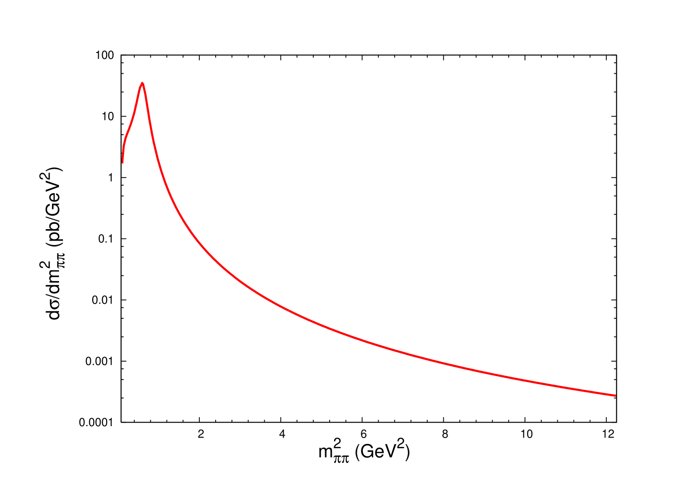
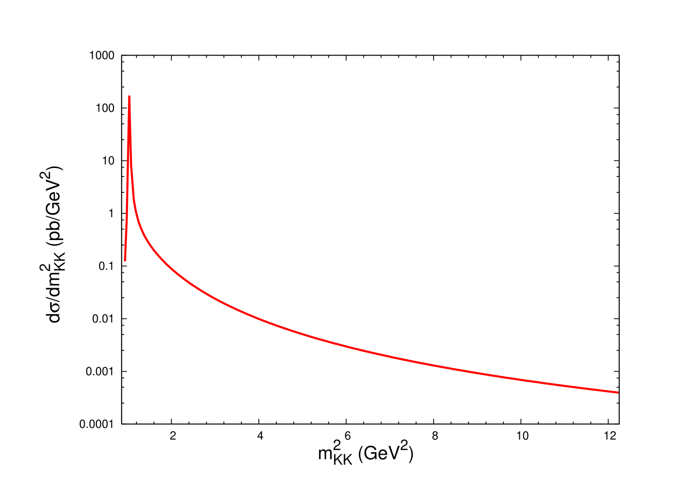
We take as the dominant background for $\Upsilon(1S)\to\gamma S\to\gamma\pi^{+}\pi^{-}$ the radiative return process $e^{+}e^{-}\to\gamma\gamma^{*}\to\gamma\pi^{+}\pi^{-}$ and similarly for the background to $\Upsilon(1S)\to\gamma S\to\gamma K^{+}K^{-}$. We use vector meson dominance to write the pion and kaon electromagnetic form factors as

with $N_{\rho\pi}=1$, $N_{\omega\pi}=N_{\phi\pi}=0$, $N_{\rho K}=1/2$, $N_{\omega K}=1/6$, and $N_{\phi K}=1/3$. The differential cross sections, $d\sigma/dm_{\pi\pi}$ and $d\sigma/dm_{KK}$, are plotted in Figs. 10 and 11.

We can perform a similar analysis of the radiative return background to pion and kaon pairs to set a lower limit on the observable values of ${\cal B}(\Upsilon\to\gamma S){\cal B}(S\to\pi^{+}\pi^{-})$ and ${\cal B}(\Upsilon\to\gamma S){\cal B}(S\to K^{+}K^{-})$. These are plotted in Figs. 12 and 13.

We can then use Eq. (4) with the branching ratios of $S$ obtained from Eqs. (18) and (20) to translate the branching ratio limits to limits on observable values of $\lambda_{d}$. We use the same naive efficiency and resolution as in the pseudoscalar analysis. The limits that come from $\gamma\mu^{+}\mu^{-}$, $\gamma\pi^{+}\pi^{-}$, and $\gamma K^{+}K^{-}$ final states will depend on the value of $r=\lambda_{u}/\lambda_{d}$. These limits, for several values of $r$, are plotted in Figs. 14-16.

We observe that the limit due to the pion final state becomes more stringent as $r$ is increased. For $r>1$ the dimuon final state does not offer very useful bounds and the hadronic final states become more important.

For large $m_{\pi\pi}$ or $m_{KK}$, the background is suppressed since the electromagnetic form factors are far from resonance. Thus, we see that we can probe down to smaller couplings than in the dimuon case where the increased resolution becomes a limiting factor. At large enough $m_{\pi\pi}$ or $m_{KK}$, we do not expect any background. Requiring that we see three signal events limits $\lambda_{d}\mathrel{\hbox to0.0pt{\lower 4.0pt\hbox{\hskip 1.0pt$\sim$}\hss}\raise 1.0pt\hbox{$>$}}0.2$. This can be thought of as an absolute lower bound on observable values of the coupling.

Assuming that the dominant background is due to the radiative return process, the minimum coupling that can be probed in both the scalar and pseudoscalar cases scales as

where $N$ is the number of quarkonia produced, $\sigma$ is the cross section of the radiative return background, $\int{\cal L}~dt$ is the integrated luminosity, and $\epsilon$ is the efficiency. At a given $q^{2}$, $\sigma\sim\hat{s}^{-1}=M_{V}^{-2}$, where $M_{V}$ is the mass of the resonance. Then the minimum coupling scales as $(\epsilon M_{V}^{2}N^{2}/\int{\cal L}~dt)^{-1/4}$.